Design issues in adaptive control - Automatic Control ... - IEEE Xplore

50

IEEE TRANSACTIONS ON AUTOMATIC CONTROL, VOL. 33, NO. 1, JANUARY 1988

Design Issues in Adaptive Control RICHARD H. MIDDLETON, GRAHAM C. GOODWIN, FELLOW, IEEE,DAVID J. HILL, DAVID Q . MAYNE, FELLOW, IEEE

Abstract-The contributions of this paper are in two main areas. The first is an integrated approach to the design of practical adaptive control algorithms. In particular, we bring many existing ideas together and explore the effect of various design parameters available to a user. Secondly, we extend the theory by showing how the problem of stabilizability of the estimated model can be overcome by running parallel estimators. We also show how asymptotic tracking of deterministic set points can be achieved in the presence of unmodeled dynamics.

1. INTRODUCTION

A

GENERAL problem in control theory is to design control laws which achieve good performance for any member of a specified class of systems. Various strategies have been proposed for achieving this result. For example, robust controllers [11-[3] are aimed at achieving good performance for the class of systems which are close (in a well-defined sense) to some fixed nominal system. Adaptive controllers are a special class of nonlinear control laws which are intended to stabilize all members of a wider class of systems, namely those systems which are close to any member of a given set of nominal systems, e.g., those nominal systems having some fixed McMillan degree [4]. Adaptive controllers generally have the additional property that the detailed structure of the control law can be decomposed into an on-line parameter estimation module together with an on-line control law synthesis procedure [4]-[6]. The first stability results for adaptive controllers were obtained in the late 1970’s. At this time several research groups (see, for example, [7]-[ 121) published results which established global convergence for a class of model reference adaptive control laws applied to linear minimum-phase plants of known order. Subsequently, the results were extended to nonminimum-phase plants provided pole-zero cancellations were avoided in the estimated model. Several methods have been proposed for achieving this, e.g., persistent excitation [ 141, restricting the parameter space to a single convex region [ 131, [ 5 ] , and searching the parameter space for suitable points [15]. These analyses were based on the assumption that the system order was equal to the assumed model order. More recently, the sensitivity of these analyses to the modeling assumptions has been questioned [161 and examples have been presented showing that the algorithms can fail if they are applied blindly to systems having unmodeled dynamics. On the other hand, there is some practical evidence [17], [18] which suggests that certain adaptive control algorithms perform well. There has been considerable research recently aimed at gaining a better understanding of adaptive control algorithms under nonideal conditions [ 191-[51]. One attractive idea that has emerged in this research is that of using either normalization or Manuscript received October 3, 1986; revised May 11, 1987. Paper recommended by Past Associate Editor, R. R. Bitmead. R. H. Middleton, G. C. Goodwin, and D. J. Hill are with the Department of Electrical and Computer Engineering, University of Newcastle, New South Wales, Australia. D. Q . Mayne is with the Department of Electrical Engineering, Imperial College of Science and Technology, London, England. IEEE Log Number 8717740.

AND

dead zones to handle disturbances and unmodeled dynamics [5], [MI, [54]-[58]. This work is a development of earlier ideas due to Egardt [52], Samson [53], and Praly [31]. It has also been incorporated in many practical realizations of adaptive control laws [18], [59]. The present paper builds on this line of research and brings together a range of techniques relevant to the design of adaptive control algorithms. Some of the techniques that are drawn upon include normalization or dead zones [5], [ U ] , [54]-[58], regression vector filtering [60], [71], pole-assignment [5], [13], [14], internal model principle adaptive control [5], [61], and least squares [5], [61]. A discussion of convergence issues is presented for the resulting algorithm and this is related to design considerations. In particular, we show how pole-zero cancellations in the estimated model can be avoided, e.g., by running parallel estimators; and we show how asymptotic tracking of a desired set pointy* is achievable for plants having unmodeled dynamics. Our analysis shall be presented in the continuous-time domain. The reasons for doing this are: first the analysis then applies, with minor modification, to the discrete case also and, second, this gives confidence in the performance when rapid sampling is used. In practice, one would invariably use a discrete-time implementation, in which case we suggest use of the delta operator [61], [63] which gives enhanced numerical properties.

II. THESYSTEM MODEL We consider a plant described by the following model: A d = B,u + C,v

(2.1)

where the degrees of the polynomial operators A,, B,, and C, satisfy,,a >, ,a ,a, 2; ,8 and v is a bounded term which may include noise and deterministic disturbances. We rewrite (2.1) by introducing a nominal transfer function, Ho = B / A , as Ay =Bu + q + d

(2.2)

where U , y denote the plant input and output, respectively, q denotes an unmodeled component, and d denotes a purely deterministic noise term. The polynomial operators A , B are coprime and of degree aA,,a, respectively, where a, < aA and A is monic. Remark 2.1: Models of the form (2.2) have been used extensively in the literature, e.g., in [311, [44], [501, 1701, [731. The term q includes bounded noise and unmodeled components in the system response. For example, if the plant is modeled in transfer function form as y=[Ho(l +A)+R]u where Ho = B / A , H = B/A, and H = q=

[x + x ] BB AB

U.

(2.3)

B/A,then (2.4) VVV

The deterministic component of the noise d is assumed to

OO18-9286/88/0lOO-OO50$01.OO 0 1988 IEEE

51

MIDDLETON er al. : DESIGN ISSUES IN ADAPTIVE CONTROL

parameters. Note that e* is not required to be unique and, in general, will not be. The filtering operation outlined above is crucial to the success Sd=O (2.5) of adaptive controllers since it focuses the parameter estimator on where S is a known monic polynomial of degree a, having the relevant frequency band thereby significantly reducing the nonrepeated zeros on the stability boundary. For example, if d is a deleterious effects of unmodeled dynamics and disturbances. In sinewave of angular frequency wo, then S = D2 + w $ D = d / some cases this may be sufficient to obtain satisfactory performdt. ance. For example, robust stability has been established under Finally, to ensure that the final control system based on the these conditions provided persistently exciting signals are added internal model principle is well posed, we require the following. [34], [36], [40], [46], [47], [60],and [71]. However, in many Assumption A.1: S has no zeros in common with the cases, it is impractical to add these signals and thus a separate line numerator Bo of the true plant transfer function Bo/Ao. V V V of development has evolved to treat this case. A key feature of this development has been the incorporation of additional normalization or dead zones into the parameter estimator to reduce the In. PARAMETER ESTIMATION estimator gain when the unmodeled response is large. This line of We now introduce a bandpass fiiter to eliminate the determinis- development can be traced to early work on bounded disturbances tic disturbance and also to mitigate the effect of unmodeled of Egardt [ll], Samson [53], and later to Praly [74] who treated dynamics on the estimator. This is a combination of the ideas in, the case of unmodeled dynamics. This idea has also been for instance [60], [61], and [71]. We define the following filtered investigated in [311, [MI, [501, [53], 1571, 1581, 1611, [MI, [701, variables: [72], and [76]. A key feature of the above development has been the introduction of overbounding functions for the unmodeled reGS - GS y = - y ; U=(3.1) sponse. This is possible provided the unmodeled response is stable JQ JQ in the sense made precise below. where G, J, Q are monic Hurwitz polynomials a, = a, and a, = Assumption A.2: The filtered unmodeled error q ~ ithe s sum of a bounded term, plus a term related to 12 by a strictly proper a., exponentially stable transfer function. VVV Using (3.1) and (2.51, the model (2.2) can be rewritten as The following result then establishes the fact that { (rlf(t)(}is Ay= Bti + q (3.2) overbounded by a function { p ( t ) }which depends on past values of la(t)l and lu(t)l. where Lemma 3. I: For all members of the class of systems satisfying Assumption A.2 there exist constants uo E (0, l), eo 2 0, E 2 0, GS q=T). (3.3) and a constant vector U such that JQ (3.12) 1 ?)J(t)1 5 E&) + eo for all t Equation (3.2) will, in general, be unsuitable for parameter estimation since the equation error term i j involves differentia- where tion of the unmodeled error which may include noise. We, (3.13) p(t)= sup {I v Tx(7)Ie- O O ( ~ - r ) ] therefore, introduce an additional filter, 1/E, where E is monic, OSTSI Hurwitz, and aE = a., We then define the following: x is the following state vector: (3.4) x 4 [Dn+s+&'-IZ' f , * . * , z ; , D " - ' u ~ , ufIT (3.14) satisfy a model of the form

a..,

Substituting (3.4) into (3.2) gives

and

y = ( E - A ) y f + B u j + VJ.

(3.5)

4 FQz; 1

z;

z 4 y-y*.

(3.15)

This equation can be expressed in regression form as =

ve*+ VJ.

(3.6)

Note that in (3.6), we have ignored initial condition terms which decay exponentially fast to zero due to the stability of F = EJ. They can be treated without further difficulty as in [lo] and [61. In (3.6) (with n P a,, m 4 a, s 2 a, g P )a, the various terms are dT=[yj,

'

OT=[eo-ao,

0

.

.a.,

)

D"-'YJ, U/

D"uJ]

en-'-an-', bo,

..a,

b,]

(3.8)

(3.9) (3.10)

B ( D ) P b , D m + b , - I D m - ' + . . . + b o.

(3.11)

In some earlier papers, e.g., [29] f?* has been called the tuned

Vuf+(bounded terms).

(3.16)

Then, if we define U = [O,

*

. 0,

1,

U,-Z,

*

., v,]

it follows that VuJ = uTx. The remainder of the proof is straightforward as in [5, Appendix B]. VVV Remark 3. I: Other bounding functions can be used [311, [U], [50], [57] in place of p(t), e . i . , based on weighted integrals of ~ X t letc. . vvv --,-,, In our subsequent analysis we will replace knowledge of { q f( t ) }by any suitable overbounding function p(t). We therefore introduce the following assumption. Assumption A.3: Constants eo, E , U , uo are assumed known vvv such that (3.12) is satisfied. ~

A ( D ) 4 D"+a,-lD"-'+ * * . + a0

[3+3] BB AB

VJ=

(3.7)

where E(D) 4 D"+e,-,D"-'+.*.+e0

Proof (Outline): We introduce an arbitrary Hurwitz polyno+- ~ v,ofdegreen - 1 . Inview mial V = D"-' + U , , - ~ D " of (2.4), vJ can then be expressed as

52

IEEE TRANSACTIONS ON AUTOMATIC CONTROL,

We next propose the following parameter estimator: = bP4e

DP= - b P + $ T P + R ; P(0)=P(O)T>O

(3.17)

R=R~ZO

VI b($- e 2 )

(3.28)

~b((~p+e~)~-e~)

(3.29)

where we have used (3.12). Using the expression for b in the case of dead zones (3.24), we then have

(3.20)

and where b represents a time-varying gain. The basic idea in both normalization and dead zones is to reduce b when the unrnodeled dynamics are large. In the case of normalization one may use b=

1, JANUARY 1988

Proof (Outline): Consider the “Lyapunov” function V = 8TP-18 with 8 = 8 - e*. Then

(3.18) (3.19)

VOL. 33, NO.

(3.30) since s = 0 when e2 I P2(ep + [see (3.22)]. Now in view of (3.22), (3.23); se2 = f e 2 f 2 and thus

QI

1+a2p2+4TP4

(3.21)

(3.31) where cyI, a2 > 0 are constants, chosen such that aldcy2and aleO are small. Note that in this case the algorithm does not depend VVV The remainder of the proof follows as in [ 5 ] , [ 6 ] . explicitly on knowledge of E or eo. Remark 3.3: This lemma is an extension to the continuous-time In the case of a dead zone, we select 0 > 1, and define VVV least-squares case of results in [43], [50], and [ S I . Lemma 3.3 (Normalization): Consider the parameter estima0 if I d t ) I I P ( ~ p ( t+) €01 (3.22) tor (3.17), (3.18), (3.21) applied to any system of the form (2.1), s(t) P subject to Assumption A.3. Then the following properties hold f ( P [ ~ p ( t+)E O ] , e ( t ) ) / e ( t )otherwise irrespective of the control law: where e-g

if e > g

i)

e+g ife 0 such that

Q, the corresponding model is uniformly

VQV

0

-90 -1,-

-Pn+g+s-l

In (5.1) we have allowed the desired closed-loop polynomiaJ to depend upon the parameter estimates. (Hence, the notation A*.) We require the following condition. Assumption A.4: The partial derivative ad*/a$is bounded and A * is uniformly strictly Hurwitz. QVV A key technical point is that we must ensure that all limit points of the algorithm correspond to a stabilizable model. Several techniques have been proposed in the literature for achieving this. One method is the use of parameter space search techniques as suggested in, for example, [15], [72], and [76]. Another method involves constraining the parameter estimates to a single convex region in which the tuned parameters lie and such that all models in the region are stabilizable [5], [6], [13], [50]. Here we extend the latter strategy to include any finite union of convex sets which satisfies Assumption A.4. Assumption A S : There exists a finite set ( D , , ., D p ) of convex sets (not necessarily disjoint) such that

60-

-?o

-Cn+g+s-l

zi=(E-L^)uf-pz;

j ( t )= j ( t o )

for all r 2 to.

54

IEEE TRANSACTIONS ON AUTOMATIC CONTROL, VOL. 33, NO.

ii) With the time origin moved to to, then

for some co, c1, U

1, JANUARY 1988

> 0, and thus

f E Lz and @ E L2. proofi In view of Assumption A S it is clear that there exists a j such that e* E D; From Lemma 3.2 it follows that Mj is bounded. The result then follows since the algorithm ensures Mj(f) IMj

+ y.

vvv

Properties of the homogeneous part of (6.1) are given in the following. Lemma 6.2: Consider the following homogeneous linear timevarying system:

DZ(t)=A( t ) Z ( t ) . Provided i) A ( t ) is bounded.

ii)

' ;1

Using Gronwall's lemma we then have

IIA(r)I12drskOt+kl; \It, Twhere ko is

sufficiently small. iii) The eigenvalues of A are strictly inside the stability boundary for all t. Then (6.6) is exponentially stable. Proof (Outline): (See also [431, [MI, 1571, [651, [ X I , and [76] for closely related results.) Choose I' = r T 1 0 and let Q(t) denote the positive definite symmetric solution to

A =(t)n(t)+ o(t)A( t )= - r

(6.7)

then using i)-iii) we can show that Q(t)is uniformly positive definite, bounded, and 3 k2 s.t. Il~(t)II2~kzIlft(t)112.

(6.8)

Now consider the system 1 D( w(t))= ( A( t )- j0-'(t)O(t))w(t)

(6.9)

V ( t )= w = ( t ) Q ( fw) ( t )

(6.10)

P(t)= - W T ( t ) r W ( t )

(6.1 1)

and define

sc0lln(~)ll3 exp (clk;kl)exp (koclkict- r)). (6.16) From (6.16), it is clear that provided ko < a/clk;, (6.6) is exponentially stable. vvv Remark 6.1: Lemma 6.2 is useful in the analysis of adaptive controllers employing either relative dead zones or normalization. In the case of relative dead zones, property ii) of Lemma 3.2 implies that koin Lemma 6.2 is zero. In the case of normalization, property ii) of Lemma 3.3 implies that ko is nonzero in vvv general. We will now illustrate the stability analysis of the adaptive algorithm for the case of dead zones. Theorem 6. I (Dead Zones): 1) Subject to Assumptions A. 1-A.5 and provided E [in (3.12)] is sufficiently small, then the adaptive control law, applied to the plant (2.2), is globally stable in the sense that y and U (and, hence, all states) are bounded for all finite initial states and any bounded Y*. 2) If, in addition, y* is purely deterministic, satisfying Sy* = 0, and €0 = 0, it then follows that lim J y ( t )-y*(t) I = 0.

[EP + €01. The algorithm ensures there are no finite escapes. We then redefine the time origin as to = 0 where to is as in Lemma 5.1. l)-Noting that the eigenvalues of A (t) are the 2n + g + s zeros of A* and in view of Assumption A.4 ii), it follows that the conditions of Lemma 6.2 are satisfied. From (6.7)

we then have = 4 4 , O)x(O) +

which establishes exponential stability of (6.9). Rewriting (6.6) gives 1 1 D Z ( t ) = ( A ( t ) - - Q-'(t)O(t))Z(t)+- Q-'(t)8(t)Z(t).(6.12) 2 2

The solution to (6.12) can be written Z(t)=&t,

1'

T)Z(T)+

$(t,

1

5 n - ' ( r ) h ( ~ ) Zdr (~)

7)

$4,7)81(e(r)+ r(r))d7

(6.18)

where 4(tl T ) is the state transition matrix corresponding to A (t). In view of Lemma 6.2 and since rand xo are bounded, we have

for some ko, kl, U > 0. From (3.23), and using Schwarz's inequality, it follows that

(6.13)

where &t, 7) is the state transition matrix of the system in (6.9). In view of the exponential stability of 6 established in (6. lo), (6.1 l), and using Schwarz's inequality, we have IIZ(t) 112IC@-2"(r- T)IIX(T)

(6.17)

Proof: The proof is based on (t.1). The various terms in this equation are dealt with as follows: A (t) is exponentially stable; r is bounded and thus a BIBS argument can be used; e can be decomposed into a sum of terms in f and e - f; the term in f is dealt with by Gronwall's lemma sincef E Lz; and the term in e - f is handled by a small gain type argument since le - f I < 0

(6.20)

1; (6.21) (6.14)

55

MIDDLETON et al. : DESIGN ISSUES IN ADAPTIVE CONTROL

where we have used (3.13). Since the right-hand side of (6.21) is monotonic nondecreasing in t , it follows that

Using (6.31) in (6.29) we have

Since the right-hand side of (6.32) is monotonic nondecreasing in t , and kl~Pllu(l< A, we then have

Then provided E < u//klPJlulI, we can show that

(6.33) and thus Since f E Lz (Lemma 3.2) and 1(4(~)115 Ilx(~)Il,it follows using Gronwall's lemma that x(t) is bounded. x bounded implies 4, p , e bounded, and thus D x is bounded in view of (6.1). Thus, 22 and y are bounded. To show U is bounded we use Assumption A . l , i.e., S and B, are coprime polynomials. If we take A : Hurwitz and of the same degree as A,, then G S / J Q and B J A ; are coprime in the ring of rational, stable, proper transfer functions [66]. That is, there exist stable, proper, transfer functions x, A such that

Thus, from (3.13), it follows that p ( t ) + 0. Since f E Lzand Dfis bounded, we have f ( t ) + 0. So e(t) 0 and from (6.1) we have --+

lim ( D x ( t ) ) = 0.

(6.25) (6.26)

(6.35)

lim x ( t ) = 0. I-m

1-m

(6.36)

From (6.36) and (6.35) it follows that z(t) = y ( t ) - y*(t) +

vvv

0.

VII. DISCUSSION OF DESIGN PARAMETERS

or (6.27) and thus U is bounded, since U, y , and v are bounded. 2) Equation (6.1) holds in this case also, however, since Sy* = 0, we have r = 0 in view of (6.5); and since 4 is bounded (as established in I), f E L2 implies f E Lz. We then have

CI

(6.29) and so we select h The result in part 1) relied on E < u/kIP(lu(l; such that 0 < ekIP((uI(< h < U. We now rearrange the third term on the right-hand side of (6.29) as: c,

(6.31) (where X, = min

{(U

- A),

UO}).

The adaptive control law depends on the following user choices:

A* the orders of A and B the internal model polynomial S the estimator filter the sampling rate the details of the least-squares algorithm the choice of the overbounding functions the method of dealing with model stabilizability. Clearly, the choice of A* is influenced by the_de_siredclosedloop bandwidth. We have made A* a function of A , B since this is essential in practice. For example, the st_ablewell damped part o,f B should be cancelled, i.e., included in A * . The unstable part of B places an upper bound on the achievable bandwidth; a sensible choice being to reflect the unstable zeros through the imaginary axis. The part of A which is not stable and well damped places a lower limit on the bandwidth. When these various requirements conflict, one is faced with a very difficult control problem and one ought to investigate alternative architectures including additional measurements if possible. The choice of orders of A , B is a compromise between reducing the potential unmodeled dynamics, on the one hand, and increased complexity including additional burden on the parameter estimator and possible model stabilizability difficulties on the other hand. In many practical cases, a third-order model is adequate. The internal model polynomial S will almost always include integral action. This is essential to eliminate load disturbances, input offsets, etc. One should only attempt to cancel sinewave type disturbances if they are well within the achievable closedloop bandwidth. If an internal model polynomial is used, then it is desirable to place stable zeros in A * near the zeros of S , this being the classical equivalent of having an integral bandwidth well below the system bandwidth. In fact, for the case of ordinary

.

56

IEEE TRANSACTIONS ON AUTOMATIC CONTROL, VOL. 33, NO. 1 , JANUARY 1988

integral action, this separation in bandwidths implies that one can do the control system design without considering the integrator and then to retrofit the integrator with a suitably small gain. The stability analysis can be readily extended to cover this procedure-see [77] for further details. The prime function of the estimator filter is to focus the parameter estimator on an appropriate bandwidth. There are two aspects, namely high-pass filtering to eliminate d.c. offsets, load disturbances, etc., and low-pass filtering to eliminate irrelevant high frequency components including noise and system response. The net effect is a bandpass filter. The rule of thumb governing the design of the filter is that the upper frequency should be about twice the desired system bandwidth and the lower frequency should be about one tenth the desired bandwidth. The choice of sampling rate is uncontroversial, it should be, if at all possible, ten times the maximum system bandwidth. The key requirement on the least-squares parameter estimator is that an upper and lower limit be placed on the algorithm gain. The exact choice of gain represents a compromise between rapid tracking of time-varying parameters and smoothing of the noise. Further discussion is given in [78]-[81]. In the choice between normalization and dead zones, one consideration is that dead zones require knowledge of the size (i.e., constants E , eo) of the errors. On the other hand it has the advantages over normalization of directly bounding the estimates, of ensuring that the parameters do not drift leading to potential bursting phenomena, and of giving zero tracking errors in the presence of unmodeled dynamics. It would seem that, in practice, some combination of dead zones and normalization would give best performance. The choice of constants (U, uo, eo, E ) in the overbounding function p is problem dependent. In view of (3.16), V plays the role of an additional filter prior to the signal entering p . This filter should also be linked to the closed-loop bandwidth, and will normally have small d.c. gain. The choice of a. depends on the damping of the unmodeled dynamics. Finally, there are a number of ways of dealing with the problem of stabilizability of the estimated models. We have introduced multiple convex regions as one way of dealing with the problem. In some cases, the choice of these regions is straightforward, e.g., when the model is of low order. In other cases, some sort of prior knowledge will be crucial in overcoming the problem.

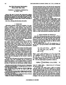
VIII. EXPERIMENTAL RESULTS The theory, as outlined above, has been implemented in a practical adaptive controller [59]. This adaptive controller has been found to give excellent performance under a wide range of experimental conditions. For example, on electromechanical servo systems, we have been able to make 2000 percent step changes in gain, time constant, and d.c. offset and yet retain excellent closed-loop performance. Fig. 1 shows a typical set of results obtained on a Feedback Ltd. ESlB Servo kit. The desired output y*, was a square wave of amplitude +30° and period 1 second; the sampling rate was 50 Hz, the desired closed-loop polynomial was A* = (0.076 + l)3; the parameter estimator was a constant trace version of leastsquares incorporating a relative dead zone; G / F was chosen as an all pole second-order low-pass filter of bandwidth 15 Hz; S / Q was chosen as 616 + 1 to eliminate d.c. offsets in U ; and an integrator was retrofitted to the system. These choices are in accordance with the guidelines given in Section VII. For the results in Fig. 1, the gain of the servo was switched between 5 and 100 percent as indicated by the arrows. The lower trace shows the estimate of this gain. The upper trace shows the output response of the servo system. IX. CONCLUSIONS This paper has discussed design issues in adaptive control. The theoretical results have been supported by experimental evidence

Fig. 1. Adaptive control of servo system. Upper trace: system response. Lower trace: estimate of system gain (6,). t 20: I gain increase. 120: 1 gain decrease.

of the claimed robustness properties. We believe that the success of the algorithm is a result of the judicious amalgamation of various techniques including regression vector filtering, pole assignment, choice of desired closed-loop polynomial as a function of estimated model. estimator dead zone, least-squares, internal model principle’. REFERENCES J. C. Doyle and G. Stein, “Multivariable feedback design: Concepts for a classical modern synthesis,” IEEE Trans. Automat. Contr., vol. AC-25, pp. 4-16, 1981. G . Zames and B. A. Francis, “Feedback, minimax sensitivity and optimal robustness,” IEEE Trans. Automat. Contr., vol. AC-28, pp. 586-601, 1983. B. R. Barmish, “Necessary and sufficient conditions for quadratic stabilization of an uncertain linear system,” J. Optimiz. Theory Appl., 1985. K. J. Astrom, “Theory and applications of adaptive controlsurvey, Automatica, vol. 19, no. 5, pp. 471-487, 1983. G. C. Goodwin and K. S. Sin, Adaptive Filtering, Prediction and Control. Englewood Cliffs, NJ: Prentice-Hall, 1984. G . C. Goodwin and D. Q. Mayne, “A parameter estimation perspective of continuous time adaptive control,” Automatica, 1987. A. Feuer and A. S. Morse, “Adaptive control of a single input single output linear system,” IEEE Trans. Automat. Contr., vol. AC-23, pp. 557-570, 1978. G. C. Goodwin, P. J. Ramadge, and P. E. Caines, “Discrete time multivariable adaptive control,” IEEE Trans. Automat. Contr., vol. AC-25, pp. 449456, 1980. K. S. Narendra, Y. H. Lin, and L. S. Valavani, “Stable adaptive controller design, Part 11: Proof of stability,” IEEE Trans. Automat. Contr., vol. AC-25, pp. 4 4 0 4 9 , Mar. 1980. A. S., ,Morse, “Global stability of parameter-adaptive control systems, IEEE Trans. Automat. Contr., vol. AC-25, no. 3, pp. 433439, 1980. B. Egardt, “Stability analysis of discrete time adaptive control schemes,” IEEE Trans.Automat. Contr., vol. AC-25, pp. 710-717, 1980. K. S. Narendra and Y. H. Lin, “Stable discrete adaptive control,” IEEE Trans. Automat. Contr., vol. AC-25, pp. 456-461, 1980. G. Kreisselmeier, “An approach to stable indirect adaptive control,” Automatica, vol. 21, no. 4, pp. 425433, 1985. H. Elliott, R. Christi, and M. Das, “Global stability of adaptive pole placement algorithms,” IEEE Trans. Automat. Contr., vol. AC-30, pp. 348-357, Apr. 1985. Ph. delarminat, “On the stabilization condition in indirect adaptive control,” Automatica, vol. 20, no. 6, pp. 793-796, 1984. C. Rohrs, L. Valavani, M. Athans, and G. Stein, “Robustness of adaptive control algorithms in the presence of unmodeled dynamics,” IEEE Trans. Automat. Contr., vol. AC-30, pp. 881-889, Sept. 1985. K. J. Astrom, “Analysis of Rhors counterexamples to adaptive control,” in Proc. 22nd Conf. Decision Contr., San Antonio, TX, 1983. B Wittenmark and K. J. Astrom, “Practical issues in the implementation of self-tuning control,” Automatica, vol. 20, pp. 595-606, Sept. 1985. P. J. Gawthrop and K. W. Lim, “Robustness of self-tuning controllers,” Proc. IEE, vol. 129, pp. 21-29, 1982. P. Ioannou and P. V. Kokotovic, “Robust redesign of adaptive control,” IEEE Trans. Automat. Contr., vol. AC-29, pp. 202-21 1, 1984.

MICIDLETON et al.: DESIGN ISSUES IN ADAPTIVE CONTROL

1211 R. L. Kosut and B. Friedlander, “Robust adaptive control: Conditions for global stability,” IEEE Trans. Automat. Contr., vol. AC-30, pp. 610-624, July 1985. G. Kreisselmeier, “On adaptive state regulation,” IEEE Trans. Automat. Contr., vol. AC-27, pp. 3-17, 1982. R. Ortega and I. D. Landau, “On the model mismatch tolerance of various parameter adaptation algorithms in direct control schemes. A sectoricity approach,” presented at the IFAC Workshop on Adaptive Contr., San Francisco, CA, 1983. B. D. 0. Anderson and R. M. Johnstone, “Adaptive systems and time varying plants,” Int. J. Contr., vol. 37, pp. 367-377, 1983. P. A. Ioannou and P. V. Kokotovic, “Adaptive systems with reduced models,” Lecture Notes in Control and Information Sciences, Vol. 47. New York: Springer-Verlag, 1983. B. D. 0. Anderson and R. M. Johnstone, “Robust Lyapunov results and adaptive systems,” in Proc. 20th IEEE Conf. Decision Contr., San Diego, CA, 1981. B. D. 0. Anderson, “Exponential convergence and persistent excitation,” in Proc. 21st IEEE Conf. Decision Contr., Orlando, FL, 1982. K. S. Narendra and A. M. Annaswamy, “Persistent excitation and robust adaptive algorithms,” presented at the 3rd Yale Workshop on Appl. of Adaptive Syst., New Haven, CT, 1983. R. L. Kosut and B. Friedlander, “Performance robustness properties of adaptive control systems,” in Proc. 21st IEEE Conf. Decision Contr., Orlando, FL, 1982. R. L. Kosut, C. R. Johnson, Jr., and B. D. 0. Anderson, “Robustness of reduced-order adaptive model following,” presented at the 3rd Yale Workshop on Adaptive Syst., 1983. L. Praly, “Robustness of indirect adaptive control based on pole placement design,” presented at the IFAC Workshop on Adaptive Contr., San Francisco, CA, June 1983. B. D. Riedle, B. Cyr, and P. V. Kokotovic, “Disturbance instabilities in an adaptive system,” IEEE Trans. Automat. Contr., vol. AC-29, pp. 822-824, 1984. B. D. Riedle and P. V. Kokotovic, “A stability instability byndary for disturbance free slow adaptation and unmodeled dynamics, presented at the 23rd Conf. Decision Contr., Las Vegas, NV, 1984. B. D. Riedle and P. V. Kokotovic, “Integral manifolds and slow adaptation,” Univ. Illinois, Tech. Rep. DC-87, Oct. 1985. I. M. Y. Mareels and R. R. Bitmead, “On the dynamics of an equation arising in adaptive control,” in Proc. 25th Conf. Decision Contr., Athens, Greece, 1986, pp. 1161-1 166. R. L. Kosut and B. D. 0. Anderson, “Robust adaptive control: Conditions for local stability,” in Proc. 23rd Conf. Decision Contr., Las Vegas, NV, Dec. 1984. 2.J. Chen and P. A. Cook, “Robustness of model reference adaptive control systems with unmodeled dynamics,” Int. J. Contr., vol. 39, no. 1, pp. 201-214, 1984. M. Bodson and S. Sastry, “Exponential convergence and robustness margins in adaptive control,” in Proc. 23rd Conf. Decision Contr., Las Vegas, N V , Dec. 1984. K. S. Narendra and A. M. Annaswamy, “Robust adaptive control in the presence of bounded disturbances,” Yale Univ., New Haven, CT, Rep. 8406, 1984. L. C. Fu, M. Bodson, and S. S. Sastry, “New stability theorems for averaging and their applications to the convergence analysis of adaptive identification and control schemes,” Univ. Calif., Berkeley, Mem UCB/ERL M85/21. B. D. 0. Anderson, R. R. Bitmead, C. R. Johnson, Jr., and R. L. Kosut, “Stability theorems for the relaxation of the strictly positive real condition in hyperstable adaptive schemes,” presented at the 23rd Conf. Decision Contr., Las Vegas, NV, 1984. C. F. Mannerfelt, “Robust control design with simplified models,” Ph.D. dissertation, Lund, 1981. L. Praly, “Robust model reference adaptive controllers, Part 1: Stability analysis,” in Proc. 23rd Conf. Decision Contr., Las Vegas, N V , Dec. 1984. P. A. Ioannou and K. Tsakalis, “Robust discrete-time adaptive control,” IEEE Trans. Automat. Contr., vol. AC-31, pp. 10331043, Nov. 1986. R. L. Kosut and C. R. Johnson, Jr., “An input-output view of robustness in adaptive control,” Automatica, vol. 20, no. 5, pp. 569581, 1984. R. Bitmead and C. R. Johnson, Jr., “Discrete averaging and robust identification” in Control and Dynamic Systems, Vol. XXXIV, C. T. Leondes, Ed. P. Kokotovic, B. Riedle, and L. h a l y , “On a stability criterion for continuous slow adaptation,” Syst. Contr. Lett., vol. 6, pp. 7-14, 1985. B. D. Riedle and P. V. Kokotovic, “Stability analysis of an adaptive system with unmodeled dynamics,” Int. J. Contr., vol. 41, no. 2, pp. 389-402, 1985. J. M. Krause, M. Athans, S. Sastry, and L. Valavani, “Robustness studies in adaptive control,” in Proc. 22nd Conf. Decision Contr., San Antonio, TX, 1983.

57 [SO] G. Kreisselmeier, “A robust indirect adaptive control approach,” Int. J. Contr., vol. 43, no. 1, pp. 161-175, 1986. [51] K. S. Narendra and A. M. Annaswamy, “Robust adaptive control using reduced order models,” in Proc. 2nd IFAC Workshop on Adaptive Syst., 1986, pp. 49-54. 1521 B. Egardt, Stability of Adaptive Controllers. New York: SpringerVerlag, 1979. C. Samson, “Stability analysis of adaptively controlled systems subject to bounded disturbances,” Automatica, vol. 19, pp. 81-86, 1983. B. B. Peterson and K. S. Narendra, “Bounded error adaptive control,” IEEE Trans. Automat. Contr., vol. AC-27, pp. 1161-1168, 1982. J. M. Martin-Sanchez, “A globally stable APCS in the presence of bounded noise and disturbances,” IEEE Trans. Automat. Contr., vol. AC-29, pp. 461-464, 1984. A. L. Bunich, “Rapidly coverging algorithm for the identification of a linear system with limited noise,” Automat. Remote Contr., vol. 44, no. 8 , part 2, pp. 1049-1054, Aug. 1983. G. Kreisselmeier and B. D. 0. Anderson, “Robust model reference adaptive control,” IEEE Trans, Automat. Contr., vol. AC-31, pp. 127-133, 1986. G. C. Goodwin, R. Lozano Leal, D. Q. Mayne, and R. H. Middleton, “Rapprochement between continuous and discrete model reference adaptive control,” Automatica, vol. 22, no. 2, pp. 199-208, Mar. 1986. G. C. Goodwin, “UNAC-The University of Newcastle adaptive controller,” University of Newcastle, N.S.W., Australia, Tech. Rep., June 1985. C. R. Johnson, Jr., B. D. 0. Anderson, and R. R. Bitmead, “Improving the robustness of adaptive model-following via information vector filtering,” Tech. Rep. ANU, 1984. G. C. Goodwin, “Some observations on robust estimation and control,” plennary address, 7th IFAC Symp. Identification, York, 1985. C. A. Desoer and C. A. Lin, “Tracking and disturbance rejection of MIMO nonlinear systems with PI controller, ” IEEE Trans. Automat. Contr., vol. AC-30, pp. 861-867, 1985. [631 R. H. Middleton and G. C. Goodwin, “Improved finite word length characteristics in digital control using delta operators,” IEEE Trans. Automat. Contr., vol. AC-31, Nov. 1986. I641 C. E. de Souza, G. C. Goodwin, D. Q. Mayne, and Palaniswami, “An adaptive control algorithm for systems having unknown time delay,” submitted for publication. C. A. Desoer, “Slowly varying discrete system x,,, = A,x,,” Electron. Lett., vol. 6, May 1970. C. A. Desoer, R.-W. Liu, and R. Saeks, “Feedback system design: The fractional representation approach to analysis and synthesis,” IEEE Trans. Automat. Contr., vol. AC-25, no. 3, pp. 399-412, 1980. R. H. Middleton and G. C. Goodwin, “On the robustness of adaptive controllers using relative deadzones,” presented at the 1987 IFAC World Congress. 1681 P. J. Gawthrop, “Self-tuning PID controllers: algorithms and implementation,” IEEE Trans. Automat. Contr., vol. AC-31, pp. 201209, Mar. 1986. I691 C. J. Harris and S. A. Billings, Self-Tuning and Adaptive Control: Theory and Applications. New York: Peregrins, 1981. 1701 L. Praly, “Global stability of a direct adaptive control scheme with respect to a graph topology,” in Adaptive and Learning Systems: Theory and Applications, K. S. Narendra, Ed. New York: Plenum, 1986. B. D. 0. Anderson, R. R. Bitmead, C. R. Johnson, Jr., P. V. 1711 Kokotovic, R. L. Kosut, I. M. Y. Mareels, L. Praly, and B. D. Riedle, Stability of Adaptive Systems: Passivity and Averaging Analysis. Cambridge, MA: M.I.T. Press, 1986. P. delarminat, “Explicit adaptive control without persistently exciting 1721 inputs,” presented at the 2nd IFAC Workshop on Adaptive Syst. in Contr. and Signal Processing, Lund, July 1986. R. Ortega, L. Praly, and I. D. Landau, “Robustness of discrete time direct adaptive controllers,” IEEE Trans. Automat. Contr., vol. AC-30, pp. 1179-1187, Dec. 1985. L. Praly, “MIMO stochastic adaptive control: Stability and robustness,” Ecole des Mines Fontainebleau, France, CAI Rep., Mar. 1982. C. Samson, “Problemes en identification et commande des systemes dynamiques,” These d’Etat, University de Rennes, 1983. P. delarminat, “Unconditional stabilization of linear discrete systems via adaptive control,” Syst. Contr. Lett., July 1986. A. Feuer and G. C. Goodwin, “Integral action in robust adaptive control,” Faculty of Elect. Eng., Technion, Israel Inst. Technol., Haifa, Israel, Tech. Rep. 1781 T. R. Fortescue, L. S. Kershenbaum, and B. E. Ydstie, “Implementation of self tuning regulators with variable forgetting factors,” Automatica, vol. 17, pp. 831-835, 1981. I791 E. Fogel and Y. F. Huang, “On the value of information in system identification-Bounded noise case,” Automatica, vol. 18, no. 2, pp. 229-238, 1982. 1801 M. E. Salgado, G. C. Goodwin, and R. H. Middleton, “A modified least squares algorithm incorporating exponential resetting and forget-

58

IEEE TRANSACTIONS ON AUTOMATIC CONTROL, VOL. 33. NO, 1, JANUARY 1988

ting,” Dep. Elect. Comput. Eng., Univ. Newcastle, N.S.W., Australia, Tech. Rep. EE8708, 1987. [811 R. Kulhary and M. Karny, “Tracking of slowly varying parameters by directional forgetting,” in Proc. 9th IFAC Congress, 1984, pp. 7883.

Richard H. Middleton was born in Waratah, Australia, on December 10, 1961. He received the B.Sc. and B.E. (Hons. I) degrees from the University of Newcastle, New South Wales, Australia, in 1984 and 1985, respectively, and the Ph.D. degree in 1987. He is currently a Lecturer in the Department of Electrical and Computer Engineering, University of Newcastle, where his interests include adaptive control, computer control systems, and electronics.

Graham C. Goodwin (M’74-SMW-F’86) was born in Broken Hill, Australia, in 1945. He received the B.Sc. degree in physlcs, the B.E. degree in electrical engineering, and the Ph.D. degree from the University of New South Wales, New South Wales, Australia. From 1970 until 1974 he was a Lecturer in the Department of Computing and Control, Imperial College, London, England. Since 1974 he has been with the Department of Electrical and Computer Engineering, University of Newcastle, New South Wales, Australia. He is the coauthor of three books: Control Theory (London: Oliver and Boyd, 1970), Dynamic System Identification (New York: Academic, 1977), and Adaptive Filtering, Prediction and Control (Englewood Cliffs, NJ. Prentice-Hall, 1984). Dr. Goodwin is a member of the Australian Research Grants Comnuttee.

David J. Hill received the B.E. degree in electrical engineering and the B.Sc. degree in mathematics from the University of Queensland, Australia, in 1972 and 1974, respectively, and the Ph D. degree in electrical engineering from the University of Newcastle, New South Wales, Australia, in 1976. He is currently a Senior Lecturer in Electrical and Computer Engineering at the University of Newcastle. Previous appointments include research positions in the Electronics Research Laboratory, University of California, Berkeley, from 1978 to 1980 and a Queen Elizabeth 11 Research Fellowship at the University of Newcastle from 1980 to 1982. During 1986 he occupied a Guest Professorship in the Department of Automatic Control, Lund Institute of Technology, Lund, Sweden. His research interests are mainly in nonlinear systems and control, stability theory, and power system stability and security. Dr. Hill is a member of I.E. Australia, the Society for Industrial and Applied Mathematics, and the International Conference on Large Electric High-Tension Systems.

David Q. Mayne (S’75-SM’77-F’81) was born in South Africa and received the B.Sc. and M.Sc. degrees in engineering from the University of Witwatersrand and the Ph.D. and D.Sc. degrees from the University of London. During the period 1950 to 1959 he held the posts of Lecturer at the University of Witwatersrand and, for two years, Research and Development Engineer at the British Thomson Houston Company, Rugby, England. Since 1960 he has been with the Imperial College of Science and Technology, London, England. He became a Reader in 1967 and a Professor in 1971. He was a Visiting Research Fellow at Harvard University in 1971, and has spent several summers at the University of California, Berkeley, in collaborative research with Professor E. Polak. He is the joint author, with D. H. Jacobson, of Differential Dynamic Programming (New York: Elsevier) and joint Editor, with R. W. Brockett, of Geometric Methods in System Theory (Dordrecht: Reidel). He is an Associate Editor of the Journal of Optimization Theory and Applications. His major research interests are in optimization, computer-aided design, and adaptive estimation and control. Dr. Mayne is a Fellow of the IEEE and the Institute of Electrical Engineers and a member of the Mathematical Programming Society. He was recently elected a Fellow of the Royal Society. He was also awarded a Senior Science Research Council Fellowship for the period 1979 to 1980.