Design Manifolds Capture the Intrinsic Complexity and ... - Umd
Recommend Documents
interior length of the cochlea are related by dilation. ... where ââ¦â denotes composition of functions and where convolution â is with respect to time, is a ... With effective implementation in mind, we have revisited WAM with Baccala and Cri
The second common property of these theories is that each example is trivial and strongly ... D. (This property depends only on the theory of A. An element a â A is algebraic ... An infinite family F of finite subsets of Ï is an almost everywhere.
theorem and a higher G-signature theorem for Lipschitz manifolds. ..... is a dense *-subaIgebra of A, stable under hotomorphic functional calculus. Proof. It's clear ...
Jan 15, 2009 - two-bridge knots and links, torus knots, some pretzel knots, and some theta-graphs. Using modified Heegaard complexity, we obtain upper.
Performance of the proposed algorithms is investigated and compared by several ... I. INTRODUCTION. Linear Blind Source Separation (BSS) addresses the prob- .... of measuring diagonality of matrices, namely, the off-norm function [13] and ...
Marketing and sales. Organization and processes. Assets and resources along the value .... Look for ways to standardize
Dept. of EECS (m/c 154), University of Illinois at Chicago, 851 S. Morgan St. - 1120 SEO, Chicago, IL. 60607-7053 ... The lower bounds above hold for nonrecursive r.e. sets A as well. ..... (In the definition above, C stands for characteristic.
Engineering Design: The Department of Mechanical Engineering invites applications for a fullâtime, tenureâtrack facu
Engineering Design: The Department of Mechanical Engineering invites applications for a fullâtime, tenureâtrack facu
2. Show that if A is context free then SUBSEQ(A) is context free. 3. Show that if A ... a computable function that does the following: Given a context-free grammar.
Our work is based on a remarkable theorem of Higman ... SUBSEQ(A) = {x ∈ Σ∗ : (∀z ∈ S)[z ≼ x]}. (1). The original proof of this ... ples”) of a c.e.3 language in some arbitrary order, and the learner must ..... Given DFAs F and G, one can effectively
Richard Beigelâ. University of Illinois at Chicago. William Gasarchâ . University of Maryland. Martin Kummerâ¡. Universität Chemnitz-Zwickau. Georgia Martin§.
TODD A. DRUMM AND WILLIAM M. GOLDMAN. Abstract. Complete flat Lorentz 3-manifolds with nonamenable fundamental group bear a striking resemblance ...
3.12 of the ANSI/ISA-RP 12.6-1987 as any device which will neither generate nor
store more than 1.2 volts, 0.1 amps, 25 mW or 20 µJ. Examples are simple ...
(1) Closed manifolds admitting a Riemannian metric whose scalar curvature ... M cannot be embedded in a closed manifold) can be deduced from this case.
http://www-edc.eng.cam.ac.uk/people/cme26.html ... designers may not have predicted how changes would propagate across the design from one part to ..... Consequence Software Development: an Empirical Study', ISSC'03, Ottawa, Canada.
Tampa, FL , 33620, USA. And. William F. Murphy, Jr. IS/DS, University of South ..... factor and elegance was Apple's iPad. The reasoning approach that seems ...
Massachusetts Institute of Technology (MIT) ... approaches to the SE process because of AAS program complexity and difficulty, and ..... Automotive News: 8.
Aug 6, 2001 - (8) for every integer M N. Iterating now these relations we obtain (7). ... choices correspond to using a single windowed WH frame WHgo o ...... THEOREM 5 Suppose the matrices W(s) and M(t)N(t) are strictly positive ...... a lower bound
For class 1 the elliptic fibration is replaced with the distinguished complex analytic foliation ~(X) given above, and the cones are again just the foliation currents ...
Keywords: intrinsic safety; HAZOP; hydrogenation unit; safety design. 1. ... And the hydrogenation unit design will be taken as an example to introduce the ...
a whitening step as a pre-process to reduce the dimensionality of observations, might be seriously limited due to its blind trust on the data covariance matrix.
Peter Robinson at the University of Hull and Henry. Merryweather of RADAN Computational Limited for their assistance and invaluable advice. This research.
Design Manifolds Capture the Intrinsic Complexity and ... - Umd
Jonah Chazan. Department of Computer Science ... This paper answers those questions by proposing methods to study design embeddings. ... In engineering optimization, the number of design variables severely impacts .... a multidimensional parameter space in R6 with parameters (a,b,m,n1,n2,n3) [1] in Eqn. (1). With a ...
Design Manifolds Capture the Intrinsic Complexity and Dimension of Design Spaces Wei Chen∗
Mark Fuge
Department of Mechanical Engineering Department of Mechanical Engineering University of Maryland
Jonah Chazan Department of Computer Science University of Maryland College Park, MD 20742 Email: [email protected]
ABSTRACT This paper shows how to measure the intrinsic complexity and dimensionality of a design space. It assumes that high-dimensional design parameters actually lie in a much lower-dimensional space that represents semantic attributes—a design manifold. Past work has shown how to embed designs using techniques like autoencoders; in contrast, the method proposed in this paper first captures the inherent properties of a design space and then chooses appropriate embeddings based on the captured properties. We demonstrate this with both synthetic shapes of controllable complexity (using a generalization of the ellipse called the superformula) and real-world designs (glassware and airfoils). We evaluate multiple embeddings by measuring shape reconstruction error, pairwise distance preservation, and captured semantic attributes. By generating fundamental knowledge about the inherent complexity of a design space and how designs differ from one another, our approach allows us to improve design optimization, consumer preference learning, geometric modeling, and other design applications that rely on navigating complex design spaces. Ultimately, this deepens our understanding of design complexity in general.
∗ Corresponding
MD-16-1647
author.
W. Chen, M. Fuge, and J. Chazan
1
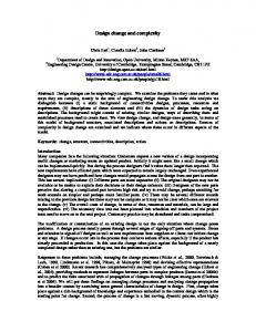
Fig. 1: 3D visualization of high dimensional design space showing that design parameters actually lie on a 2-dimensional manifold.
1
Introduction Products differ among many design parameters. For example, a wine glass contour can be designed using coordinates
of B-spline control points: with 20 B-spline control points, a glass would have at least 40 design parameters. However, we cannot arbitrarily set these parameters because the contour must still look like a wine glass. Therefore, high-dimensional design parameters actually lie on a lower-dimensional design manifold (Fig. 1) or semantic space that encodes semantic design attributes, such as roundness or slenderness. A manifold’s intrinsic dimension is the minimal dimensionality we need to faithfully represent how those high-dimensional design parameters vary. Past researchers, both within and beyond design, have proposed many algorithms for mapping high-dimensional spaces to lower dimensional manifolds and back again—what we call a design embedding. But how do you ensure the embedding has captured all the geometric variability among a collection of designs, while not using more dimensions than necessary? How do you evaluate which embedding best captures a given design space? What properties should a good design embedding possess? This paper answers those questions by proposing methods to study design embeddings. Specifically, our method measures the complexity of a high-dimensional design space and the quality of an embedding. We demonstrate our approach on synthetic superformula examples [1] with varying complexity and real-world glassware and airfoil examples. While this paper focuses on mathematically understanding design spaces, our approach ultimately has implications for several important sub-fields of Engineering Design. In engineering optimization, the number of design variables severely impacts accuracy and convergence. In consumer preference models, high-dimensional design spaces complicate capturing human opinion inexpensively or accurately. In design interfaces, designers have difficulty exploring and manipulating highdimensional design spaces. Because our approach automatically determines a design space’s complexity and dimension, these sub-fields can assess 1) their task’s fundamental difficulty, and 2) how to best reduce that difficulty. Mathematically, our work deepens our understanding of design complexity in general by illuminating how design embeddings model a design space, how to judge the inherent complexity of a design space, and how to measure the ways designs differ from one another. MD-16-1647
W. Chen, M. Fuge, and J. Chazan
2
Our main contributions are: 1. A method for embedding designs in the fewest dimensions needed to control shape variations. 2. A minimal set of performance metrics for embeddings, including reconstruction error, topology preservation, and whether the manifold captures key shape variations. 3. Manifold benchmarks with controllable complexity (i.e., non-linearity, dimensionality, and separability) for testing design embeddings.
2
Related Work Past research has taken two different approaches to understanding design spaces and synthesizing new shapes or
designs—knowledge-driven methods and data-driven methods [2]. Knowledge-driven methods generate new shapes or designs via explicit rules. One representative example is procedural modeling, which creates 3D models and textures of objects (such as buildings and cities) from sets of rules [3,4]. Another example is Computational Design Synthesis (CDS), which synthesizes designs (such as gearboxes and bicycle frames) based on topological or parametric rules or constraints [5, 6, 7, 8, 9]. However, such explicit rules are hard to specify or generalize to diverse design objectives. Data-driven methods, by contrast, learn the representation of geometric structure from examples, adjusting the model to match provided design data. We refer the readers to the survey by Xu et al. [2] for an overview of data-driven shape processing techniques. Our work uses a data-driven approach to learn the inherent complexity and the semantic representation of a shape collection, and synthesize shapes by exploring that semantic representation. Generally, there are three main data-driven approaches: 1) assembly-based modeling, where parts from an existing shape database are assembled onto a new shapes [10,11,12,13,14]; 2) statistical-based modeling, where a probability distribution is fitted to shapes in the design space, and plausible shapes are generated based on that distribution [15, 12, 16]; and 3) shape editing, where a low-dimensional representation is learned from high-dimensional design parameters, and designers create shapes by exploring that low-dimensional representation. This paper falls into that third category. Many approaches use manifold learning techniques such as Multi-Dimensional Scaling (MDS) to map the design space to a low-dimensional embedding space [17]. However such approaches generally construct only one-way mappings (high to low). Some methods can also directly learn a two-way mapping between the design space and the embedding space, such as autoencoders, which using neural networks to project designs from high to low dimension and back again [18, 19]. Another way is to associate shapes with their semantic attributes by crowd-sourcing, and then learn a mapping from the semantic attributes to the shapes, such that new shapes can be generated by editing these semantic attributes [20].
3
How Our Contributions Relate to Prior Work Our hypothesis is that while shapes are represented in a high-dimensional design space, they actually vary in a lower-
dimensional manifold, or surface within the larger design space [21, 22]. One would then navigate a shape space by moving across this manifold—like an ant walking across a surface of a sphere—while still visiting all valid designs. This raises several questions: How does one find the manifold (if it exists)? How does one “jump back” to the high-dimensional space MD-16-1647
W. Chen, M. Fuge, and J. Chazan
3
(raw geometry) once one has wandered around on the manifold? How does one choose a “useful” manifold, and how does ones evaluate that “usefulness?” A common issue for previous shape synthesis methods is that they often do not address the inherent properties (e.g., intrinsic dimension, non-linearity) of the geometric design space before embedding, choosing instead to set parameters (such as dimensionality) manually. This causes problems during embedding and shape synthesis because this may not adequately capture shape variability or may use unnecessary dimensions along which designs do not vary. Unlike past work, this paper directly investigates the inherent complexity of a design space under the assumption that different parts of that space may differ in complexity. We discover information such as discontinuities in the design space and the intrinsic dimension of each segment. We then adjust the embeddings and design manifolds based on that information. Another issue is that given various embeddings (constructed by MDS, autoencoders, etc.), how does one choose the embedding that best enables a smooth and accurate exploration of the space? Reconstruction error is one common metric for evaluating embeddings. It measures how accurately the model can reconstruct input data as it embeds data from high dimension to low and back again. However, sometimes embeddings can excel at reconstruction but ultimately place the data in a lower-dimensional space with unexpected and unintuitive topological structures, such as linear filaments in Deep Autoencoders [23]. While these structures may aid accurate reconstruction, they make it difficult for users to explore the embedded space. In this paper, we propose evaluation metrics that measure three properties of an embedding: (1) its reconstruction accuracy, (2) how well it preserves a design space’s topology, and (3) whether it captures the design space’s principal semantic attributes. In practice, there is often a trade-off between these metrics, and our approach allows a designer to visualize and decide among embeddings with respect to that trade-off. Past research has also studied various theoretical bounds on the performance of different dimensionality reduction techniques [24, 25, 26]. However, current analytical results apply largely to cases where the mapping is linear and performance is measured in terms of Euclidean distances. In this paper, we consider a broader class of manifolds that include non-linear mappings and non-Euclidean distances. We direct interested readers to Sec. S1 in the supplementary material for a review and discussion of the available theoretical results.
4
Samples and Data Before we discuss our approach, we need to introduce some concrete benchmarks of design spaces that we will demon-
strate and validate our method over. By design space, we mean any M-dimensional vector (x ∈ RM ) that controls a given design’s form or function—e.g., its shape, material, power, etc. To create a high-dimensional design space X , we generate a set of design parameters or shape representations X ∈ X . For ease of explanation and visualization, this paper uses designs described by 2D curved contours, however the proposed methods extend to non-geometric design spaces as well, as we show (i)
in Sec. S8. Specifically, we uniformly sample points along the shape contours and use their coordinates as X where x j and MD-16-1647
W. Chen, M. Fuge, and J. Chazan
4
Fig. 2: Examples of superformula shapes. (i)
y j are the x and y coordinates of the jth point on the contour of the ith sample:
The sample shapes come from two sources: 1) the superformula [1] as a synthetic example whose design space space complexity we can directly control; and 2) glassware and airfoil contours as real-world examples.
4.1
Synthetic Benchmark Since this paper’s goal is to capture a design space’s inherent properties, we first need a benchmark dataset whose
properties we can directly control; this allows us to measure performance with respect to a known ground truth. Since, to our knowledge, no such benchmark exists for design embeddings, we created one using a generalization of the ellipse—called the superformula (See Fig. 2 for examples)—that allows us to control the following properties: (non-)Linearity, number of separate manifolds, intrinsic dimension, and manifold separability/intersection. Two-dimensional superformula shapes have a multidimensional parameter space in R6 with parameters (a, b, m, n1 , n2 , n3 ) [1] in Eqn. (1). With a radius (r) and an angle (θ), the superformula is expressed in polar coordinates as:
r(θ) =
! 1 cos( mθ ) n2 sin( mθ ) n3 − n1 4 4 + a b
(1)
thus the Cartesian coordinates X are:
(x, y) = (r(θ) cos θ, r(θ) sin θ)
4.1.1
Controlling Linearity
By tuning the parameters in Eq. 1 we can vary the non-linearity of X; for example, by changing the aspect ratio s of the shapes, we can linearly vary X:
(x, y) = (s · r(θ) cos θ, r(θ) sin θ) MD-16-1647
W. Chen, M. Fuge, and J. Chazan
(2) 5
Abnormal! m=5
m=3 m=4
(a) Linear design space (d = 1) varying s.
(b) Nonlinear space (d = 2) varying s & n3 .
(c) Design space with multiple shape categories.
Fig. 3: 3D visualization of the superformula design space created by a linear mapping from the high-dimensional design space X to a 3-dimensional space, solely for visualization. Each point represents a design.
We can control the linearity of X by tuning the linear switch s in Eqn. (2) or the nonlinear switches {a, b, m, n1 , n2 , n3 } in Eqn. (1). Fig. 3a and 3b are examples of controlling linearity of the design space. A design space’s linearity is reflected by the curvature of the manifold—higher non-linearity results in higher curvature.
4.1.2
Controlling the Intrinsic Dimension
To artificially control the intrinsic dimension M of the design space, we construct M-dimensional subspaces of the superformula parameter space by varying M parameters choosing from {s, a, b, m, n1 , n2 , n3 }, and keeping other parameters fixed, as shown in Fig. 3a (1-D) and 3b (2-D).
4.1.3
Controlling the Number of Shape Categories
A collection of designs does not always consist of just one category of shapes. For example, a collection may contain not only glassware, but also bottles, which have very different contours to glassware and likely have different manifold properties. A na¨ıve embedding, which lumps glasses and bottles together, should perform poorly here, and thus we need our synthetic benchmark to create similar cases with distinct manifolds. It is possible to have multiple categories of superformula shapes by discretely changing the value of m in Eqn. (1). Because the parameter m controls the period of the right-hand-side function in Eqn. (1), we can use it to set the superformula to a m-pointed-star, as shown in Fig. 3c. The discrete change of m forms separate clusters or sub-manifolds in the design space. Another benefit of this formulation is that we can control the separability of the sub-manifold, since we can make these clusters intersect one another (e.g., Fig. 7b). We can generate intersecting clusters by setting the ranges of varying parameters n2 and n3 , such that all the clusters contain ellipses or circles. Because this superformula benchmark can generate design manifolds with many different properties, we believe it should be useful not only for benchmarking and improving future design embedding techniques, but also for evaluating manifold learning techniques in general. MD-16-1647
W. Chen, M. Fuge, and J. Chazan
6
4.2
Real-World Data
4.2.1
Glassware
Glassware is a good real-world example because 1) shape representation using B-splines smoothly fits the glass contours, and 2) we can interpret the semantic attributes of glassware—e.g., roundness, slenderness, type of drink, etc. We use 128 glass images, including wine, beer, champagne, and cocktail glasses. We fit each glass contour with a B-spline, and build the design space X using the coordinates of points uniformly sampled across the B-spline curves.
4.2.2
Airfoils
An airfoil is the cross-section shape of a wing or blade (of a propeller, rotor, or turbine). Like glassware, we can also represent airfoils via 2D contours and they have discernible semantic attributes that allow us to verify different embeddings. A good airfoil shape embedding can aid airfoil optimization; for example the proposed method can provide a continuous space with the fewest number of necessary dimensions for an airfoil optimization algorithm to optimize over, improving convergence speed and accuracy. Our airfoil samples are from the UIUC Airfoil Coordinates Database, which provides the Cartesian coordinates for nearly 1,600 airfoils.1 We use linear interpolation to ensure that each airfoil has the same number of coordinates in the design space X .
5
Methodology First, we try to achieve good design embeddings by understanding the complexity or properties of the design space—for
example, detecting the number of sub-manifolds and what their dimension might be. Based on those results, we then apply embeddings of appropriate complexity and type to the different sub-manifolds. We will review the high-level details of our methodology, however, some of the specific mathematical, algorithmic, and computational complexity calculations have been omitted due to space limitations; interested readers can review the online supplemental material as well as the full source code for needed to reproduce all detail in this paper.2
5.1
Pre-processing Our raw data may come from shapes with various height and width, or have inconsistent or very high dimensionality.
These issues obstruct manifold learning and embedding. We apply two pre-processing steps to mitigate these issues: Shape Correspondence We ensure that the coordinates for all designs correspond to consistent cardinality and areas in space. This step is important for our techniques to work well, however, the choice of correspondence technique is not central to the contributions of the paper. See Sec. S2 in the supplemental material for full details. Linear Dimension Reduction Before performing non-linear dimension reduction, we first use Principal Component Anal0
ysis as a linear mapping ( f 0 : X ∈ RD → X 0 ∈ RD ) to reduce X such that it retains 99.5% of the variance. See Sec. S3 in the
Learning Design Space Properties If designs do lie on manifolds, we first need to know the number, intrinsic dimension, and complexity of those manifolds
for two reasons. First, knowing the intrinsic dimension M sets the dimensionality d of the semantic space F . Setting d < M makes it impossible to completely capture all semantic attributes of designs; while d > M introduces unnecessary dimensions along which designs do not vary—this unnecessarily impedes exploration or optimization. Second, separating different categories of designs helps exclude invalid designs. To illustrate this point, we can first look into the case when there are multiple manifolds in a design space, as shown in Fig. 3c. Suppose we treat these multiple manifolds as one, and perform embedding and shape synthesis. We have to use a 3-dimensional semantic space to completely capture the variation between the designs. Since there are no design samples in between two manifolds—what we call a design cavity, we do not know whether a design from that area is valid. Consequently in that area we might synthesize a new shape which looks like a weird hybrid of two designs from two different manifolds, like the abnormal shape in Fig. 3c. In contrast, if we separate these manifolds and then do embedding and shape synthesis on each manifold/design category, we can avoid generating invalid new designs.3 For the above reasons, we apply clustering and intrinsic dimension estimation over the dimensionality-reduced design space X 0 before embedding designs.
5.2.1
Clustering
In this section we introduce an adaptive clustering method that automatically captures the number of groups given a collection of designs and then separates these groups. This method uses spectral clustering, where data are clustered using eigenvectors of an affinity matrix [27]. The affinity matrix gives pairwise similarity measures between data points. We adapted a method that is better suited for clustering manifolds, where the similarity measure considers both pairwise distances and principal angles between local tangent spaces [28]. To compute the local tangent spaces, we use an adaptive neighborhood selection algorithm to get the local data matrix. After computing the affinity matrix, we apply a method that automatically detects the number of groups and separate them using the computed affinity matrix [29]. Affinity matrix To separate manifolds, we use a method based on robust multiple manifolds structure learning (RMMSL) [28]. It assumes that within each cluster, samples should not only be close to each other, but also form a flat and smooth manifold. A manifold can be flat and smooth if it has small curvature everywhere. The method thus constructs an affinity matrix which incorporates both pairwise distance and a curvature measurement, which is computed via principal angles between local tangent spaces. See Sec. S4 in the supplemental material for further algorithmic and computational complexity details. Neighborhood Selection To compute the curvature measurement, we need the neighboring point set N(x) for each sample point x. We use the neighborhood contraction and expansion algorithm proposed by Zhang et al. [29]. The basic idea is that the neighborhood size k selected for each point x should not only reflect the local geometric structure of the
3 An
astute reader may notice that designs “off-the-manifold” may be, in some sense, creative or innovative. We return to that discussion in Sec. 6.3.
MD-16-1647
W. Chen, M. Fuge, and J. Chazan
8
manifold, but also have enough overlap among nearby neighborhoods to allow local information propagation. See Sec. S5 in the supplemental material for further algorithmic and computational complexity details. Group Number Estimation Normally given the correct number of manifolds C (i.e., group number), RMMSL has good performances in separating them [28]. However, it requires manually specifying the number C. To automatically detect the group number C, we apply a method based on self-tuning spectral clustering (STSC) [30]. This method automatically infers C by exploiting the structure of the eigenvectors V of the normalized affinity matrix A (i.e., the Laplacian matrix) using an iterative algorithm (with T number of iterations). See Sec. S6 in the supplemental material for further algorithmic and computational complexity details. In sum, we first obtain the nearest neighbors N(xi ) for each sample xi , then apply RMMSL to compute the affinity matrix W . Finally, we use W as the affinity matrix for STSC to determine the group number C and assign samples to different groups. The general computational cost for all these steps is O(N 3 ) when the sample size N is large; see Sec. S7 in the supplemental material for further discussion of when this might be cost-prohibitive.
5.2.2
Intrinsic Dimension Estimation
Following the manifold clustering procedure, we apply intrinsic dimension estimation over each manifold/design category. The estimator is based on the local dimension estimation method mentioned in RMMSL [28]. We first obtain the K nearest neighbors of each sample xi . We set the neighborhood size K using the adaptive method proposed in [31]. With the neighbors of xi and a weight matrix S, we construct a local structure matrix:
Ti = (Xi − xi 1T )SST (Xi − xi 1T )T
where S is a diagonal matrix and can be set as S j j = 1/(σ2n + σ2 α(kxi j − xi k2 )), σ2n and σ2 indicate the scales of the noise and the error, and α(·) is a monotonically non-decreasing function with non-negative domain (e.g., a quadratic) [28]. The local intrinsic dimension di is estimated from the eigenvalues of Ti —similar to dimensionality estimation using PCA. A category’s overall intrinsic dimension is the mean intrinsic dimension of all points in that category. In practice, point-wide intrinsic dimension can be noisy (and thus appear to change dimensionality often). We apply a kernel density smoother to local dimensionality estimates to account for our assumption that the local dimensionality should not vary drastically within a neighborhood on a smooth manifold. For example, if the local dimensionality estimations for xi and its five neighbors are {2, 3, 2, 2, 2, 2}, the second estimation is likely to be incorrect. After applying KDE, the new estimations will be {2, 2, 2, 2, 2, 2}. We use the Epanechnikov kernel to limit density estimation to a local neighborhood, and set the kernel bandwidth adaptively based on the distance between each sample and its Kth neighbor. MD-16-1647
W. Chen, M. Fuge, and J. Chazan
9
Invalid!
(a) Create a convex hull of the training set in the (b) Copy the boundary of the convex hull to the grid of semantic space. new designs generated from the semantic space.
(c) Remove designs outside the boundary.
Fig. 4: Set boundary of the feasible semantic space.
5.3
Embedding and Shape Synthesis We used methods involving PCA, kernel PCA (with a RBF kernel) [32], and stacked denoising autoencoders (SdA) [33], 0
which all simultaneously learn a mapping f from the space X 0 to the semantic space F ( f : X 0 ∈ RD → F ∈ Rd ) and a reverse 0
mapping g from the F back to X 0 (g : F ∈ Rd → X 0 ∈ RD ) where D0 ≥ d. PCA performs an orthogonal linear transformation on the input data. Kernel PCA extends PCA, achieving a nonlinear transformation via the kernel trick [34]. The SdA extends the stacked autoencoder [35], which is an multilayer artificial neural network that nonlinearly maps X 0 and F using nonlinear activation functions [36]. We split any design data into a training set and test set. We further split the training data via 5-fold cross validation to optimize the hyperparameters using the sequential model-based algorithm configuration (SMAC) [37]. After optimizing any hyperparameters, the model trains each example with the entire training set. We test each model with the test set. After mapping from design space X 0 to semantic space F , we also need to map back to the original X from F —i.e., given certain semantic attributes, we want to generate new shapes. This is achieved by first applying mapping g, and then 0
applying g0 (g0 : X 0 ∈ RD → X ∈ RD ), which is the inverse mapping of f 0 . To visualize the mapping g0 : F → X , we uniformly sample from F , map those samples back to X to synthesize their shapes, and then plot them in Fig. 4b. Note that although we only visualize a limited number of shapes generated from the semantic space F , we can generate infinitely many shapes when continuously exploring in F . Every semantic space should have a boundary beyond which designs are not guaranteed to be valid. For example, at the top left of Fig. 4b, the glass contours on the two sides intersect. We call these infeasible shapes, i.e., shapes that are unrealistic or invalid in the real-world. To limit F to only feasible shapes, we take the convex hull of the training samples in F as shown in Fig. 4a, and set its boundary as the boundary for the feasible semantic space. We sample and synthesize shapes inside the feasible semantic space, as shown in Fig. 4c. Because training samples all have feasible shapes, any designs lying between any two training samples should be valid if the semantic space preserves the original design space’s topology (i.e., the space is not highly distorted). As a result, this method may not explore innovative, unusual designs. While this paper’s main focus is understanding the complexity of an existing design space, we discuss how to find innovative designs in Sec. 6.3. MD-16-1647
W. Chen, M. Fuge, and J. Chazan
10
A
X
B
F1
C
F2
B
A B C: reduce rim diameter increase stem diameter
Embedding 1
B
dAB
A C
A Embedding 2
dAC
C
A C B: irregular shape variation
dAC
dAB
Fig. 5: Illustration of pairwise distance preservation. Similar designs (A and B) have similar shape representations in X , thus are closer in X than dissimilar designs (A and C). We want such relation of pairwise distances to be preserved in F (i.e., dAB < dAC ) such that shapes will vary in the same manner as they do in X . 5.4
Evaluation To evaluate embeddings, we consider these questions:
1. Given known semantic attributes (e.g., roundness and slenderness), can the embedding precisely restore the original design parameters that created it? 2. Do shapes in the semantic space (F ) vary similarly compared to the original shapes in the design space (X )? 3. Does the embedding precisely capture all the attributes that control the variation of shapes? To answer these questions, we propose three metrics for comparing embeddings: 1) reconstruction error, 2) geodesic distance inconsistency, and 3) principal attributes.
5.4.1
Reconstruction Error
Reconstruction error measures how the actual design parameters X 0 differ from the design parameters of the input data once we project them onto the low-dimensional manifold and un-project back into high-dimensional space. We use the symmetric mean absolute percentage error (SMAPE) [38] to measure reconstruction error: (i)
(i)
1 m n |r j − s j | ε= ∑ ∑ (i) (i) mn i=1 j=1 |r | + |s | j
(3)
j
(i)
where m is the sample size, n is the number of design parameters for each sample, r j is the ith reconstructed design (i)
parameter for the jth sample, and s j is the ith original design parameter for the jth sample.
5.4.2
Pairwise Distance Preservation
To answer the second question, we can compare the pairwise distances of samples in the high-dimensional design space
X versus the low-dimensional semantic space F . Generally, as shown in Fig. 5, similar designs (A and B) have similar shape representations (e.g., Cartesian coordinates of shape outlines) in X , thus are closer in X than dissimilar designs (A and C). We want such pairwise distances to be preserved in F (i.e., dAB < dAC ) such that shapes will vary in the same manner as they do in X . Since we assume our samples lie on a manifold in X , we use the pairwise geodesic distances along the manifold as the pairwise distances to be preserved after the embedding. Specifically, we construct a nearest neighbor graph G over the samples X ∈ X to model the manifold structure. G is a MD-16-1647
W. Chen, M. Fuge, and J. Chazan
11
weighted graph where the edge weight between neighbors is their Euclidean distance. The nearest neighbors are selected using the neighborhood contraction and expansion algorithm mentioned in the neighborhood selection section. This algorithm adaptively chooses the neighborhood size for each sample based on its local manifold geometry. The neighborhood size is large where the manifold is flat, and small where it is curvy. Thus this method prevents “shortcuts” across high-curvature manifolds and maintains large enough overlap among nearby neighborhoods. Then we compute all pairs shortest paths for the graph G, and construct a geodesic distance matrix DG . We compare DG with the pairwise Euclidean distance matrix D of the embedded samples F ∈ F using Pearson’s correlation coefficient. The geodesic distance inconsistency (GDI) can be expressed as
GDI = 1 − ρ(DG , D)2
(4)
where ρ(DG , D) is the Pearson’s correlation coefficient between DG and D. Lower GDI indicates the embedding better preserves pairwise distances. Normally, embedding methods like Isomap will have low GDIs because they explicitly optimize pairwise distances. However, they cannot simultaneously learn two-way mappings between the design space and the embedding space. Methods like autoencoders are able to learn two-way mappings, but they usually have higher GDIs because they minimize reconstruction error rather than preserve distances. There is often a trade-off between reconstruction and distance preservation; embeddings that explicitly optimize both objectives would be an interesting topic for future research.
5.4.3
Principal Attributes
For superformula examples, we know what their correct semantic spaces should look like by looking at their parameter spaces. A parameter space P (e.g., Fig. 6a) for the superformula contains the shapes generated by all possible combinations of values for all the parameters used to modify the shapes. It is this space from which we randomly select training and testing samples. For example, if we fix parameters {a, b, m, n2 , n3 } and vary {s, n1 } in Eqn. (1) and Eqn. (2), the superformula parameter space will have two dimensions (i.e., P ∈ R2 ). Along the first dimension some shape attribute (e.g., aspect ratio) changes with s, and along the second dimension another attribute (e.g., roundness) changes with n1 . We call these attributes the principal attributes. We can also vary these two attributes along a single dimension by simultaneously varying s and n1 (e.g., let s = αt and n1 = βt, where α and β are coefficients, and t is a variable). Fig. 7a shows an example where two shape attributes vary along each dimension—the aspect ratio4 changes along one dimension and roundness along the other, and the number of arms changes over both dimensions. Because the number of arms is not continuous, the clustering algorithm should separate shapes with different number of arms. And within each cluster, a good embedding should capture the other two attributes—the aspect ratio and roundness. A good embedding should precisely capture the right principal attributes, such that tuning these attributes creates diverse
4 All
the shapes shown in the figures are scaled to the same height. Thus the aspect ratio will matter instead of the height or the width.
MD-16-1647
W. Chen, M. Fuge, and J. Chazan
12
(a) Shapes in the superformula parameter space.
(b) Generated shapes in the semantic space.
Fig. 6: An example comparing shapes generated from the semantic space F versus the superformula parameter space P . If the embedding precisely captures the principal attributes, shapes from F should look like those from P —with neither extra unexpected shape variation nor missing diversity.
(a) Shapes in the superformula parameter space.
(b) Result of manifold clustering (as in Fig. 3, the design space X is visualized in three dimensions).
(c) Generated shapes in semantic spaces. Since there are three categories, we have three separated semantic spaces.
Fig. 7: Multiple superformula categories with intersection. Our approach correctly separates the three sub-manifolds, even though they all connect via a common seam.
but valid shapes. By comparing the shapes generated from the semantic space F with those from the superformula parameter space P , we can evaluate whether the embedding precisely captures all the attributes that control the variation of shapes. That is, shapes generated from F should look similar to those from P —with neither unexpected shape variation nor missing diversity, as shown in Fig. 6.
6
Results and Discussion We evaluated our method’s performance at recovering various design space properties. We also compared how well
different embedding approaches captured shape attributes. MD-16-1647
W. Chen, M. Fuge, and J. Chazan
13
(a) Shapes in the superformula parameter space.
(b) Result of manifold clustering (as in Fig. 3, the design space X is visualized in three dimensions).
(c) Generated shapes in semantic spaces.
Fig. 8: Multiple superformula categories with intersection and different intrinsic dimensions. Our intrinsic dimension estimator automatically detects the appropriate dimensionality of the semantic space for each design category (c).
6.1
Design Space Properties We use the superformula examples to test the accuracy of our clustering algorithm and intrinsic dimension estimator.
We conducted experiments with the number of clusters C set from 1 to 5, intrinsic dimension from 1 to 3, and three levels of linearity (curvature of the manifold). All the experiments correctly separated the superformula shape categories and estimated the correct intrinsic dimensions (Fig. 7). In cases where multiple manifolds intersect (Fig. 7b), it is improper to use metrics like the rand index to evaluate clustering accuracy, because samples at the intersection can be classified to any adjacent group. For example, shapes turn into ellipses at the intersection (Fig. 7a), so it does not matter whether they belong to the four- or five-pointed star group. Figure 7c shows that our approach captures this case. Figure 8 demonstrates a case where two manifolds with different intrinsic dimensions intersect: one superformula category with a intrinsic dimension of 1 intersects with another category with a intrinsic dimension of 2. Our method correctly separates the two categories and estimates the intrinsic dimension for each category, as shown in Fig. 8c.
6.2
Principal Attributes As mentioned above, a good embedding should precisely capture the right principal attributes. For superformula ex-
amples, we check this by comparing the shapes generated from the semantic space F with those from the superformula parameter space P . For the example shown in Fig. 7, the clustering separated shapes with different number of arms, and each cluster’s embedding correctly captured the two principal attributes—aspect ratio and roundness. In Fig. 8’s example, as expected, the embedding captured the aspect ratio and the roundness attributes of the four-pointed stars, and just the roundness for the five-pointed stars. Figure 9 shows the synthesized glassware in a 3-dimensional semantic space. This embedding captured three attributes—the rim diameter, the stem diameter, and the curvature. With the variation of these three attributes, we synthesized a collection of shapes that generally covers all the training samples—wine, beer, champagne, and cocktail glasses. Similarly, the airfoil embedding shown in Fig. 10 also captured three attributes—the upper and lower surface protrusion, and the trailing edge direction. MD-16-1647
W. Chen, M. Fuge, and J. Chazan
14
Curvature
eter
Rim
diam
Stem diameter
Lower surface protrusion
Fig. 9: Synthesized glassware shapes in a 3D semantic space. The embedding captured three shape attributes—the rim diameter, the stem diameter, and the curvature.
g Trailin
direc edge
tion
Upper surface protrusion
Fig. 10: Synthesized airfoil shapes in a 3D semantic space. The embedding captured three shape attributes—the upper and lower surface protrusion, and the trailing edge direction.
For the airfoil example, the uncovered design manifold allows us to optimize airfoil shapes over this continuous lowdimensional space instead of the original geometric design space, using metamodeling techniques like Bayesian optimization. In our future work, we will compare the performance of metamodeling techniques with and without applying our dimensionality reduction method.
6.3
Are all areas on the manifold equally valid? The different shades in Fig. 7–10 represent for local density of the shape collection (i.e., training samples) distributed in
the semantic space F . At positions nearby the training samples (e.g., point A in Fig. 11), we plot the synthesized shape with a darker color. This means we are more certain of its validity because it lies closer to real-world training samples. In contrast, in locations where training samples are sparse (e.g., point B in Fig. 11), we plot the synthesized shape with a lighter color. This means we are less certain of its validity, and our model may create shapes that diverge from the training samples. In the semantic space where the training samples are absent—what we call a design cavity—new designs might be innovative or they may be unrealistic. For example, as shown in Fig. 9, inside areas where shapes have light colors, we synthesized glassware that are not similar to any of our training samples. In this case, the model generated innovative designs rather than unrealistic ones, however, to our knowledge there is no formal mathematical way of differentiating those two cases MD-16-1647
W. Chen, M. Fuge, and J. Chazan
15
B
B
A
A
(a) Arrangement of training samples in the semantic space (for simplicity, this is a 2D projection of the 3D semantic space).
(b) Synthesized shapes.
Fig. 11: Point A has high sample density, and thus higher confidence that synthesized shapes will look similar to nearby real-world samples. In contrast, point B has low sample density, and thus lower confidence but higher chance of generating an unusual or creative shape. Shade darkness correlates with higher local density.
automatically. Doing so would be a compelling topic of future research.
6.4
Sample Arrangement in Semantic Space Figure 12 shows the comparison between results obtained from different embedding methods. For this superformula
example, PCA has a high reconstruction error because the design space is nonlinear. This results in some abnormal shapes (i.e., shapes with attributes that do not exist in the parameter space in Fig. 12a) in the semantic space created by PCA (Fig. 12c). SdA and kernel PCA have similar reconstruction errors. However, the semantic space created by kernel PCA (Fig. 12d) better aligns with the original parameter space than that of SdA (Fig. 12e), because SdA generates abnormal shapes (Fig. 12e, top right). Since these abnormal shapes have light colors, we know that they are inside the design cavity; while in fact if the embedding preserved the geodesic distances between samples (i.e., low GDI), the sample arrangement should resemble that of PCA or kernel PCA, where there is no design cavity (Fig. 12c and 12d). Therefore both high reconstruction errors (e.g., PCA in this example) and high GDI (e.g., SdA in this example) can create abnormal or invalid shapes.
7
Conclusions We introduced an approach to learn the inherent properties of a design space and evaluate two-way mappings between
a design space and a semantic space. By correctly identifying the design space properties such as the number of design categories and the intrinsic dimension, one can then create an embedding that precisely captures the principal attributes of each design category, assuming that the embedding is well chosen based on the reconstruction error and the pairwise distance preservation. This means the synthesized shapes will have no unexpected shape variation, missing diversity, or repeated shapes (brought about by unnecessary dimensions). We also introduced a benchmark for rigorously testing design embeddings that accounted for non-linear, multiple (potentially intersecting) manifolds of controllable intrinsic dimension. We encourage others to use this benchmark to improve future design embeddings. While this paper mainly addressed geometric design spaces, our approach would extend to any type of design space, MD-16-1647
W. Chen, M. Fuge, and J. Chazan
16
(a) Shapes in the superformula parameter space.
(c) Embedding and shape synthesis result by PCA.
(b) Reconstruction error and geodesic distance inconsistency.
(d) Embedding and shape synthesis result by kernel PCA.
(e) Embedding and shape synthesis result by a stacked denoising autoencoder.
Fig. 12: Comparison of different embedding methods. The abnormal shapes generated by PCA and SdA are due to high reconstruction error and high GDI respectively.
including those that involve text, materials, or combinations with geometry (For an example of a combined material and geometry space, see Sec. S8 in the supplemental material). It could apply to improving interfaces that help novices explore designs, aiding high-dimensional design optimization, and helping model consumer preferences in high-dimensional design spaces. Our work’s main implication is that choosing a design embedding carries with it important choices about what you value in your semantic space: Should it reconstruct designs consistently? Should it preserve the topology of the design space? What semantic attributes should the semantic space capture? Choosing an embedding with the properties you want is not straightforward; our approach provides a principled way to compare and contrast embeddings—to help navigate those options and identify useful properties of both the embedding and your design space in general.
Acknowledgements An earlier version of this work appeared in the ASME IDETC 2016 conference [39]. We thank the reviewers of both versions for many insightful comments that substantially improved the quality and rigor of the manuscript.
References [1] Gielis, J., 2003. “A generic geometric transformation that unifies a wide range of natural and abstract shapes”. American journal of botany, 90(3), pp. 333–338. [2] Xu, K., Kim, V. G., Huang, Q., Mitra, N., and Kalogerakis, E., 2016. “Data-driven shape analysis and processing”. In SIGGRAPH ASIA 2016 Courses, ACM, p. 4. MD-16-1647
W. Chen, M. Fuge, and J. Chazan
17
[3] M¨uller, P., Wonka, P., Haegler, S., Ulmer, A., and Van Gool, L., 2006. “Procedural modeling of buildings”. In Acm Transactions On Graphics (Tog), Vol. 25, ACM, pp. 614–623. [4] Talton, J. O., Lou, Y., Lesser, S., Duke, J., Mˇech, R., and Koltun, V., 2011. “Metropolis procedural modeling”. ACM Transactions on Graphics (TOG), 30(2), p. 11. [5] Cagan, J., Campbell, M. I., Finger, S., and Tomiyama, T., 2005. “A framework for computational design synthesis: model and applications”. Journal of Computing and Information Science in Engineering, 5(3), pp. 171–181. [6] Wyatt, D. F., Wynn, D. C., Jarrett, J. P., and Clarkson, P. J., 2012. “Supporting product architecture design using computational design synthesis with network structure constraints”. Research in Engineering Design, 23(1), pp. 17– 52. [7] K¨onigseder, C., and Shea, K., 2015. “Analyzing generative design grammars”. In Design Computing and Cognition’14. Springer International Publishing, pp. 363–381. [8] Oberhauser, M., Sartorius, S., Gmeiner, T., and Shea, K., 2015. “Computational design synthesis of aircraft configurations with shape grammars”. In Design Computing and Cognition’14. Springer International Publishing, pp. 21–39. [9] K¨onigseder, C., and Shea, K., 2016. “Comparing strategies for topologic and parametric rule application in automated computational design synthesis”. Journal of Mechanical Design, 138(1), p. 011102. [10] Chaudhuri, S., and Koltun, V., 2010. “Data-driven suggestions for creativity support in 3d modeling”. ACM Transactions on Graphics (TOG), 29(6), p. 183. [11] Chaudhuri, S., Kalogerakis, E., Guibas, L., and Koltun, V., 2011. “Probabilistic reasoning for assembly-based 3d modeling”. In ACM Transactions on Graphics (TOG), Vol. 30, ACM, p. 35. [12] Kalogerakis, E., Chaudhuri, S., Koller, D., and Koltun, V., 2012. “A probabilistic model for component-based shape synthesis”. ACM Transactions on Graphics (TOG), 31(4), p. 55. [13] Chaudhuri, S., Kalogerakis, E., Giguere, S., and Funkhouser, T., 2013. “Attribit: content creation with semantic attributes”. In Proceedings of the 26th annual ACM symposium on User interface software and technology, ACM, pp. 193–202. [14] Guo, X., Lin, J., Xu, K., and Jin, X., 2014. “Creature grammar for creative modeling of 3d monsters”. Graphical Models, 76(5), pp. 376–389. [15] Talton, J. O., Gibson, D., Yang, L., Hanrahan, P., and Koltun, V., 2009. “Exploratory modeling with collaborative design spaces”. ACM Transactions on Graphics-TOG, 28(5), p. 167. [16] Fish, N., Averkiou, M., Van Kaick, O., Sorkine-Hornung, O., Cohen-Or, D., and Mitra, N. J., 2014.
“Meta-
representation of shape families”. ACM Transactions on Graphics (TOG), 33(4), p. 34. [17] Averkiou, M., Kim, V. G., Zheng, Y., and Mitra, N. J., 2014. “Shapesynth: Parameterizing model collections for coupled shape exploration and synthesis”. In Computer Graphics Forum, Vol. 33, Wiley Online Library, pp. 125–134. [18] Yumer, M. E., Asente, P., Mech, R., and Kara, L. B., 2015. “Procedural modeling using autoencoder networks”. In Proceedings of the 28th ACM User Interface Software and Technology Symposium, UIST ’15, ACM. [19] Burnap, A., Liu, Y., Pan, Y., Lee, H., Gonzalez, R., and Papalambros, P. Y., 2016. “Estimating and exploring the product MD-16-1647
W. Chen, M. Fuge, and J. Chazan
18
from design space using deep generative models”. In ASME International Design Engineering Technical Conferences, ASME. [20] Yumer, M. E., Chaudhuri, S., Hodgins, J. K., and Kara, L. B., 2015. “Semantic shape editing using deformation handles”. ACM Transactions on Graphics (TOG), 34(4), p. 86. [21] Van der Maaten, L., Postma, E., and Van den Herik, H., 2009. “Dimensionality reduction: A comparative review”. Technical Report TiCC TR 2009-005. [22] Bengio, Y., Courville, A., and Vincent, P., 2013. “Representation learning: A review and new perspectives”. Pattern Analysis and Machine Intelligence, IEEE Transactions on, 35(8), Aug, pp. 1798–1828. [23] Duvenaud, D. K., Rippel, O., Adams, R. P., and Ghahramani, Z., 2014. “Avoiding pathologies in very deep networks.”. In AISTATS, pp. 202–210. [24] Larsen, K. G., and Nelson, J., 2014. “The johnson-lindenstrauss lemma is optimal for linear dimensionality reduction”. arXiv preprint arXiv:1411.2404. [25] Bartal, Y., Recht, B., and Schulman, L. J., 2011. “Dimensionality reduction: beyond the johnson-lindenstrauss bound”. In Proceedings of the twenty-second annual ACM-SIAM symposium on Discrete Algorithms, SIAM, pp. 868–887. [26] Shawe-Taylor, J., Williams, C. K., Cristianini, N., and Kandola, J., 2005. “On the eigenspectrum of the gram matrix and the generalization error of kernel-pca”. IEEE Transactions on Information Theory, 51(7), pp. 2510–2522. [27] Ng, A. Y., Jordan, M. I., Weiss, Y., et al., 2001. “On spectral clustering: Analysis and an algorithm”. In NIPS, Vol. 14, pp. 849–856. [28] Gong, D., Zhao, X., and Medioni, G., 2012.
“Robust multiple manifolds structure learning”.
arXiv preprint
arXiv:1206.4624. [29] Zhang, Z., Wang, J., and Zha, H., 2012. “Adaptive manifold learning”. IEEE Transactions on Pattern Analysis and Machine Intelligence, 34(2), pp. 253–265. [30] Zelnik-Manor, L., and Perona, P., 2004. “Self-tuning spectral clustering.”. In NIPS, Vol. 17, p. 16. [31] Samko, O., Marshall, A. D., and Rosin, P. L., 2006. “Selection of the optimal parameter value for the isomap algorithm”. Pattern Recognition Letters, 27(9), pp. 968–979. [32] Sch¨olkopf, B., Smola, A., and M¨uller, K.-R., 1998. “Nonlinear component analysis as a kernel eigenvalue problem”. Neural computation, 10(5), pp. 1299–1319. [33] Vincent, P., Larochelle, H., Lajoie, I., Bengio, Y., and Manzagol, P.-A., 2010. “Stacked denoising autoencoders: Learning useful representations in a deep network with a local denoising criterion”. Journal of Machine Learning Research, 11(Dec), pp. 3371–3408. [34] Sch¨olkopf, B., Smola, A., and M¨uller, K.-R., 1997. “Kernel principal component analysis”. In International Conference on Artificial Neural Networks, Springer, pp. 583–588. [35] Vincent, P., Larochelle, H., Bengio, Y., and Manzagol, P.-A., 2008. “Extracting and composing robust features with denoising autoencoders”. In Proceedings of the 25th international conference on Machine learning, ACM, pp. 1096– 1103. MD-16-1647
W. Chen, M. Fuge, and J. Chazan
19
[36] Bengio, Y., Lamblin, P., Popovici, D., Larochelle, H., et al., 2007. “Greedy layer-wise training of deep networks”. Advances in neural information processing systems, 19, p. 153. [37] Hutter, F., Hoos, H. H., and Leyton-Brown, K., 2011. “Sequential model-based optimization for general algorithm configuration”. In International Conference on Learning and Intelligent Optimization, Springer, pp. 507–523. [38] Makridakis, S., 1993. “Accuracy measures: theoretical and practical concerns”. International Journal of Forecasting, 9(4), pp. 527–529. [39] Chen, W., Chazan, J., and Fuge, M., 2016. “How designs differ: Non-linear embeddings illuminate intrinsic design complexity”. In ASME International Design Engineering Technical Conferences, ASME.
MD-16-1647
W. Chen, M. Fuge, and J. Chazan
20
List of Figures Fig. 1: 3D visualization of high dimensional design space showing that design parameters actually lie on a 2-dimensional manifold. Fig. 2: Examples of superformula shapes. Fig. 3: 3D visualization of the superformula design space created by a linear mapping from the high-dimensional design space X to a 3-dimensional space, solely for visualization. Each point represents a design. Fig. 4: Set boundary of the feasible semantic space. Fig. 5: Illustration of pairwise distance preservation. Similar designs (A and B) have similar shape representations in X , thus are closer in X than dissimilar designs (A and C). We want such relation of pairwise distances to be preserved in F (i.e., dAB < dAC ) such that shapes will vary in the same manner as they do in X . Fig. 6: An example comparing shapes generated from the semantic space F versus the superformula parameter space P . If the embedding precisely captures the principal attributes, shapes from F should look like those from P —with neither extra unexpected shape variation nor missing diversity. Fig. 7: Multiple superformula categories with intersection. Our approach correctly separates the three sub-manifolds, even though they all connect via a common seam. Fig. 8: Multiple superformula categories with intersection and different intrinsic dimensions. Our intrinsic dimension estimator automatically detects the appropriate dimensionality of the semantic space for each design category (c). Fig. 9: Synthesized glassware shapes in a 3D semantic space. The embedding captured three shape attributes—the rim diameter, the stem diameter, and the curvature. Fig. 10: Synthesized airfoil shapes in a 3D semantic space. The embedding captured three shape attributes—the upper and lower surface protrusion, and the trailing edge direction. Fig. 11: Point A has high sample density, and thus higher confidence that synthesized shapes will look similar to nearby real-world samples. In contrast, point B has low sample density, and thus lower confidence but higher chance of generating an unusual or creative shape. Shade darkness correlates with higher local density. Fig. 12: Comparison of different embedding methods. The abnormal shapes generated by PCA and SdA are due to high reconstruction error and high GDI respectively.
MD-16-1647
W. Chen, M. Fuge, and J. Chazan
21
Supplemental Materials: Design Manifolds Capture the Intrinsic Complexity and Dimension of Design Spaces
S1
Past theoretical results for dimensionality reductions There are related mathematical results that address theoretical bounds on similar embeddings to those used in this pa-
per. To our knowledge, related mathematical results are restricted to two categories. First, for Euclidean pairwise distance preservation, bounds are available primarily for linear transformations (either globally or within a neighborhood) via the Johnson-Lindenstrauss lemma. Second, for reconstruction error, bounds are available for PCA and Kernel PCA, but not for most other types of dimensionality reduction techniques, including Autoencoders. For those cases, papers report experimental results in place of theoretical results. We summarize related theoretical results below. The Johnson-Lindenstrauss lemma states that given 0 < ε < 1, a set X of m points in RN , and a number n > 8ln(m)/ε2 , there is a linear map f : RN → Rn such that
(1 − ε)ku − vk2 ≤ k f (u) − f (v)k2 ≤ (1 + ε)ku − vk2
for all u, v ∈ X. Thus the JL lemma can define a lower and upper bound for the pairwise distance preservation in linear embeddings like PCA. Larsen and Nelson [1] showed that when the embedding is linear, the reduced dimensionality m given by JL lemma is optimal associated with a pairwise distance distortion factor ε. So given a reduced dimensionality m, ε will have a lower bound. Bartal et al. [2] showed that the reduced dimensionality m in JL lemma could be reduced when preserving the distances within a neighborhood (like what Locally Linear Embedding does). This might provide a lower bound for ε in nonlinear embeddings that preserve neighborhood pairwise distances. However, the pairwise distances mentioned above are Euclidean distances rather than geodesic distances which we used to measure distance preservation. In addition, the techniques used to study LLE and related embeddings do not apply to kernel PCA and autoencoders because those techniques do not form locally linear neighborhoods in the same way. Lastly, Shawe-Taylor et al. [3] gives reconstruction error bounds for kernel PCA. Since PCA is equivalent to kernel PCA with a linear kernel, these bounds can also be applied to PCA. MD-16-1647
W. Chen, M. Fuge, and J. Chazan
1
S2
Pre-Processing: Shape Correspondence In this paper, we fixed the coordinates of the start and end points, and uniformly sample a constant number of points on
the outline. Specifically,
1. For the superformula example, we set the point whose angle is 0 in the polar coordinate system as the start point, and the point which has the largest angle in the polar coordinate system as the end point; 2. For the glass example, we set the start and end point at the top and bottom of the left contour respectively; 3. For an airfoil, its outline has two curves — the upper and lower curves. We set the left and right most point as the start and end point of each curve, respectively.
Then for the superformula and glass examples, we standardized each sample such that the y coordinates are in [0, 1]; and for the airfoil example, we standardized each sample such that the x coordinates are in [0, 1]. Other shape representation schemes (e.g., different sample scheme or B-spline control points representation) may also be feasible. In this paper we didn’t address the effects of different shape representations on obtained design manifolds. However this could be an interesting future work.
S3
Pre-Processing: Linear Dimensionality Reduction The original design space X is normally high dimensional. For example, if 100 points are used to represent the contour
of each glass, we will have a 200-dimensional design space. It is difficult to learn from such a high dimensional space because of the following reasons: 1) the standard Euclidean distance metric is no longer a reliable measurement of similarity in a high dimensional space; 2) the number of samples required grows exponentially with the dimension; and 3) computing high dimensional data requires more time and resources. The first two reasons are the consequences of what is called the curse of dimensionality [4]. Despite their high dimensionality, the design parameters X are usually highly redundant. For example, in our experiments, by using principal component analysis (PCA), the 200-dimensional glassware design parameters can be reduced to 30-dimensional while still retaining at least 99.5% of the variance between designs. Therefore, our first step is to apply simple linear dimensionality reduction to map the high-dimensional design space to a lower (but still high) dimensional space:
f 0 : X ∈ RD → X 0 ∈ RD
0
where f 0 is a linear mapping and D ≥ D0 . MD-16-1647
W. Chen, M. Fuge, and J. Chazan
2
S4
Manifold Clustering: Affinity Matrix RMMSL uses a curved-level measurement R(x) to indicate curvature and flatness:
R(x) =
kθ(Ji , J)k d(xi , x) x ∈N(x)
∑
(S1)
i
where θ(Ji , J) measures the principal angle between the tangent spaces Ji at xi and J at x, which indicates the curvature of the manifold; d(xi , x) is the geodesic distance between xi and x; and N(x) is the spatial neighborhood point set for x. 0
In general, RMMSL first performs local manifold structure estimation: it estimates the local tangent space Ji ∈ RD ×di at each sample xi , where i = 1, ..., n and di is the local intrinsic dimension at xi (the method of estimating di is introduced in Sec. 5.2.2). Then it learns the global manifold structure by constructing an affinity matrix W ∈ Rn×n using both a pairwise distance kernel w1 (xi , x j ) and a curved level kernel w2 (xi , x j ):
Wi j = w1 (xi , x j )w2 (xi , x j )
(S2)
where w1 (xi , x j ) = exp(−kxi − x j k2 /(σi σ j )), w2 (xi , x j ) = exp(−θ(Ji , J j )2 /(kxi − x j k2 σ2c /σi σ j )), σi and σ j are local bandwidth [5], and σc is a coefficient to control the effect of the curved level kernel. 2 +D0 k 02 The time complexity for estimating the local tangent spaces is O(ND0 (kmax max +D )), where kmax is the maximum
neighborhood size. The complexity for computing the affinity matrix using pairwise distances and curved-level measure2 ), where d ments is O(N 2 D0 dmax max is the maximum local intrinsic dimension. Thus the overall computational cost for getting 2 + D0 k 02 2 the affinity matrix is O(ND0 (kmax max + D + Ndmax )).
S5
Manifold Clustering: Neighborhood Selection The neighborhood contraction and expansion algorithm first uses k-NN to get a neighborhood Ni of size kmax for each
point xi , and constructs a matrix Xi − x¯i 1T , where Xi = [xi1 , ..., xikmax ] and x¯i = ∑k≤kmax xik . Then it contracts Ni by removing the farthest neighbor until some preset minimal neighborhood size kmin is reached or until the following inequality holds: s
∑
(i) (σ j )2
s (i) ≤ η ∑ (σ j )2
j>di
(i)
(i)
(S3)
j≤di
(i)
where σ j is the jth singular value of Xi − x¯i 1T (σ1 ≥ ... ≥ σkmax ), di is the local intrinsic dimension of the manifold at xi , which we will introduce in the next section. and the small constant η ∈ (0, 0.5). 0
2 (k 0 D Based on [6], for N samples the algorithm has complexity O(N(kmax − kmin )kmax max + D )), when sample xi ∈ R .
MD-16-1647
W. Chen, M. Fuge, and J. Chazan
3
S6
Manifold Clustering: Group Number Estimation For each possible group number C, the STSC algorithm tries to find a rotation Rˆ such that each row in the matrix Z = VC Rˆ
has a single non-zero entry (VC is the first C columns of V ). This is achieved by minimizing a cost function: n
C
L = ∑ ∑ (Zi2j − Mi2 ) i=1 j=1
where Mi = max j Zi j . Then the best group number C is the one with the lowest cost. Once we get the optimal Z, the sample xi can be assigned to cluster c if and only if max j (Zi2j ) = Zic2 . The eigenvalue decomposition of the Laplacian matrix takes O(N 3 ) time. Given a group number C, at each iteration of the optimization, the time for computing Z via Givens rotation [7] is O(C2 (C3 + N)). Thus the total time for computing Z 3 (C3 + N)), where C is O(TCmax max is the maximum group number, and T is the number of iterations. Assigning samples max
to clusters takes O(NCmax ) time. Therefore the overall computational cost for estimating the optimal group number is 3 (C3 + N)). While the scale complexity on C O(N 3 + TCmax max is high, in practice Cmax is often a small number, so the max
complexity penalty is manageable.
S7
Manifold Clustering: Discussion of Computational Costs The optimization discussed in Sec. 5.2.1 has several steps, with the below computational complexities where N is the
number of designs, kmax and kmin are max and min neighborhood size, D0 is the reduced linear dimensional space after pre-processing, dmax is maximum local intrinsic dimension, Cmax is the maximum possible number of groups, and T is the number of iterations. 2 + D0 k 02 2 Calculating the Affinity Matrix O(ND0 (kmax max + D + Ndmax )). 2 (k 0 Neighborhood Selection O(N(kmax − kmin )kmax max + D )) 3 (C3 + N)), where the N 3 term comes from an eigendecomposition, and the Group Number Estimation O(N 3 + TCmax max
rest from computing Z via Givens rotations. In what cases does the above complexity become prohibitive? When kmax is large Since this is the neighborhood size, it is largest when a manifold is flat. Even in such cases, kmax is tends to be small, and only serves to approximate the geodesic distance, which for flat manifolds will still be reasonably well approximated without making kmax prohibitively large. When N is large As the number of designs grow, computing eigendecompositions (for both group number estimation and for Intrinsic Dimension Estimation in Sec. 5.2.2) could scale cubically in the most general implementation of eigendecomposition. In practice, this scaling may not be quite as costly because (1) the needed matrices have special structure (symmetry) that can accelerate eigendecomposition, (2) we are interested in only the largest Cmax eigenvector/value pairs, that is, iterative eigendecomposition methods can be employed (e.g., by using vanilla Krylov methods, the time MD-16-1647
W. Chen, M. Fuge, and J. Chazan
4
complexity can be reduced to O(Cmax N 2 ), though there are Krylov methods based techniques that make use of Laplacian matrix properties to further reduce the complexity), and (3) recently developed randomized algorithms for eigendecompositions would be sufficiently accurate for the problems at hand. When D0 is large This is controlled by the number of principal components kept from the pre-processing linear dimension reduction step. In our experiments on real-world samples, D0 was O(10), however for other domains it could be higher. The pre-processing step calculates the size of D0 , and can act as a check before attempting the optimization. 6 , and thus can be expensive when a design space contains a When Cmax is large Group number estimation scales with Cmax
large number of separate manifolds. In practice, we have not observed large group cardinality (typically we see O(1)) in the real-world datasets we have studied thus far, however other domains may well have large Cmax . In general cases, we have N D0 , kmax , and Cmax , thus the overall computational cost for the proposed manifold clustering method is simply O(N 3 ), or smaller if applying techniques like Krylov methods.
S8
Incorporating non-geometric design spaces The previous examples and discussion in this paper used geometric designs. What if we had other (non-geometric)
parameters, such as material or color? To test this case, we used our proposed method on a design space with both geometric and non-geometric features. Specifically, we used the glassware data, and added an extra feature, material. We set the material to be ceramic for all the stemless shapes (with a material feature represented as 0), and glass for all the stemmed ones (material feature represented as 1). The proposed method detected two groups: Group I with an intrinsic dimension of 2, and Group II with an intrinsic dimension of 3. As expected, Group I involves all the stemless shapes made from ceramic, and Group II involves all the stemmed ones made from glass. In the design synthesis step, the materials are synthesized along with shapes. Synthesized designs are labeled ceramic if its material feature is smaller than 0.5, or glass otherwise. As shown in Fig. S1, all the synthesized stemless shapes are ceramic and stemmed ones glass, which indicates that the manifolds captured the correlation between the shape and the material. As expected, for the ceramic group our approach correctly excludes the “stem diameter” dimension, estimating only two intrinsic dimensions, since (unlike in the glass group) the “stem diameter” is varying along with the “rim diameter” in the ceramic group. In our future work, we may try to apply the proposed method on purely non-geometric features. One example is to use the flow, temperature or stress field as our high-dimensional design space. Once we could reduce its dimensionality and synthesize new fields given certain conditions, we would avoid the computationally expensive numerical methods that are usually used to compute these fields.
References [1] Larsen, K. G., and Nelson, J., 2014. “The johnson-lindenstrauss lemma is optimal for linear dimensionality reduction”. arXiv preprint arXiv:1411.2404. MD-16-1647
W. Chen, M. Fuge, and J. Chazan
5
Group II
Group I
Fig. S1: Synthesized glass shapes with different materials. We add an extra feature, material, to the input data. Specifically, we set the material to be ceramic for all the stemless shapes, and glass for all the stemmed ones. The proposed method detected two groups: Group I with an intrinsic dimension of 2, and Group II with an intrinsic dimension of 3. The materials are synthesized along with shapes. The colors red and blue represent ceramic and glass respectively. [2] Bartal, Y., Recht, B., and Schulman, L. J., 2011. “Dimensionality reduction: beyond the johnson-lindenstrauss bound”. In Proceedings of the twenty-second annual ACM-SIAM symposium on Discrete Algorithms, SIAM, pp. 868–887. [3] Shawe-Taylor, J., Williams, C. K., Cristianini, N., and Kandola, J., 2005. “On the eigenspectrum of the gram matrix and the generalization error of kernel-pca”. IEEE Transactions on Information Theory, 51(7), pp. 2510–2522. [4] Bellman, R. E., 2015. Adaptive control processes: a guided tour. Princeton university press. [5] Zelnik-Manor, L., and Perona, P., 2004. “Self-tuning spectral clustering.”. In NIPS, Vol. 17, p. 16. [6] Zhang, Z., Wang, J., and Zha, H., 2012. “Adaptive manifold learning”. IEEE Transactions on Pattern Analysis and Machine Intelligence, 34(2), pp. 253–265. [7] Golub, G. H., and Van Loan, C. F., 2012. Matrix computations, Vol. 3. JHU Press.
MD-16-1647
W. Chen, M. Fuge, and J. Chazan
6
List of Figures Fig. S1: Synthesized glass shapes with different materials. We add an extra feature, material, to the input data. Specifically, we set the material to be ceramic for all the stemless shapes, and glass for all the stemmed ones. The proposed method detected two groups: Group I with an intrinsic dimension of 2, and Group II with an intrinsic dimension of 3. The materials are synthesized along with shapes. The colors red and blue represent ceramic and glass respectively.