Design of a Nanosensor Array Architecture. Wei Xu, N. Vijaykrishnan, Y. Xie and M.J. Irwin. Microsystems Design Lab. The Pennsylvania State University.
Design of a Nanosensor Array Architecture Wei Xu, N. Vijaykrishnan, Y. Xie and M.J. Irwin Microsystems Design Lab The Pennsylvania State University University Park, PA 16802, USA
{wexu,vijay,yuanxie,mji}@cse.psu.edu limited in size, array development and demonstration has been dominated by a two-level system architecture hierarchy. The first various forms of silicon-based, chemical sensor arrays are now being developed at research institutions around the world. Over the past 10-15 years, arrays have been successfully demonstrated for the discrimination of breath alcohol constituents, consumer mixtures, automotive exhaust constituents, and various water level contains the array of sensors and the second a pattern recognition engine, typically implemented in software. All raw sensor data need to be transferred to the pattern recognition or pre-processing engine. The size and power consumption required to support this traditional architecture are often prohibitive. Unlike the macroscopic counterpart, the nanowire sensor yield is currently low (about 60%), we have to come up with a methodology to make the system immune to the low yield. Overall, our research goal is to develop a low power, cost effective and fault-tolerant sensor array system which could be integrated on one chip using the advanced VLSI technology.
ABSTRACT This paper describes a nanowire sensor array architecture for high-speed, high-accuracy sensor systems. The chip has very simple processing elements (PEs) in a massively parallel architecture, in which each PE is directly connected to seven sensors. A sampling rate of 100 ns is enough to realized highspeed sensing feedback for electronic nose. We aim to create a very simple architecture, because a compact design is required to integrate as many PEs as possible on a single chip. A widely used, easy to implement estimator—minimum distance classifier is introduced to realize the pattern recognition. A sample design is implemented in VHDL and has been simulated and synthesized using TSMC 0.25 standard cell library and a commercial 0.16 standard cell library.
Categories and Subject Descriptors B7.1 [Integrated Circuits]:Types and Design Styles – advanced technologies,algorithms implemented in hardware, VLSI
General Terms
There are several technical components of an artificial nose that can be identified. These are the sensors fabrication, the alignment of the sensors, design of A/D conversion circuits to transform the sensed signals, design of pre-processing and signal processing circuits, support for pattern recognition and the overall system design. The details of the design and manufacture of nanowire sensors as well as the assembly process are beyond the scope of this work. We only provide a brief overview of the nanowire sensors and the assembly process in section 2. This paper focuses on the pre-processing circuit and the pattern recognition methods employed to help sharpen the interpretation of the signals from nanowire sensor array.
Design, Reliability
Keywords Nanowire sensor array; Pattern recognition; Electronic nose; Gas sensing; Sensor pre-processing
1. Introduction The olfactory systems of animals and humans are exceptional at detecting and classifying odors. An important current theme in sensor research is the idea of cross-reactive arrays [1]. These arrays report accurately on the concentration of analytes in complex mixtures by virtue of the varied response of different sensor elements. Due to the analogy between the multiple sensor concept and biological olfaction, these arrays are popularly called electronic noses [2].
Section 2 gives a brief introduction about the nanowire sensor array. Section 3 describes the implementation of the A/D conversion circuit. Section 4 covers architectural details of the proposed nanosensor array architecture. Section 5 describes the pattern recognition algorithm. Section 6 illustrates the operation of the whole sensor system through an example. Section 7 shows the synthesis results and the floorplan. Section 8 concludes the paper.
The use of artificial nose is a cost effective approach to the increasingly important problem of detecting hazardous emissions. For such application, it is proposed that the electronic nose would make use of an array of sensors and reside on a computer chip.
2. Nanowire Sensor System Background While many different solid state sensing principles can be applied for sensing gases, the responses examined in this study are from chemoresistive (i.e. gas-induced changes in resistance provide the response signal) nanowire sensors using chemoresistors based on SnO2. In this section, we present the background of chemoresistive sensor chemistry. The conducting polymer is grown in between highly conductive metal such as gold. The length of the polymer is in the nanometer scale. The sensitivity of the conducting polymer resistance to concentrations of gases in the sensing environment is known to be related to adsorption and
Permission to make digital or hard copies of all or part of this work for personal or classroom use is granted without fee provided that copies are raise an alarm that a leak of a particular chemical beyond a not made or distributed for profit or commercial advantage and that threshold suspected [3].the full citation on the first page. To copy copies bearisthis notice and otherwise, or republish, to post on servers or to redistribute to lists, Such a prior chipspecific could permission be placed and/or at all apotential sites for a leak, e.g. requires fee. GLSVLSI’04, Aprilpumps, 26-28, 2004, Massachusetts, USAwould be to valves, flanges, etc. Boston, The purpose of the chip Copyright 1-58113-853-9/04/0004...$5.00. pollutants2004 [4].ACM Since most current integrated sensor arrays are
298
chip area of 7x7 mm2. The digital interface takes approximately 10% of the total area for the chip.
desorption of gas on the sensor surface [8]. The level, type and rate of adsorption and desorption changes with temperature as well as the concentration of gases. At moderate concentrations, above the sensors’ noise floor and below the saturation level of the sensor, resistance is related to gas concentration as follows: 1 (1) s AC α Where Rs is the resistance of the polymer, C is the concentration of the gas and A and α are constants. The constants A and α change with type of gas and temperature of the sensor [8]. For example, the conductivity of the polymer ranges from 0.2 to 60 S/cm, depending on the dopant. In our research, we assume the temperature is fixed to the sensor’s operating point (T=300400°C) and we focus on the concentration of target gas, i.e. detecting the existence of gas.
With hundreds to thousands of sensors, the resolution of the ADC could be aggressively reduced, while still providing the desired accuracy providing proper pattern recognition algorithm. Figure 2(a) shows the 1 bit resolution A/D converter we used in the sensor array architecture. The circuit is composed of two parts 1) a current comparator which compares the current going through the nanowire (Iin) and the reference current (Iref). If the resistance of the nanowire increases above the threshold, the output signal flips high, which means the target gas is detected. The reference current could be fine-tuned to be comparable to Iin through careful sizing of the transistors 2) signal amplifier.
R =
According to the information from the teams working on the chemistry of nanowire, and the fabrication process, the yields of both nanowire and the wire alignment are currently as low as 60%. It makes sense to process only the working sensors. Thus, we propose to mark the bad sensors. The actual change of resistance (∆R) in the presence of gas is about two orders of magnitude greater than the base resistance of the nanowire (Rsensor). For example, we could design a nanowire with base resistance to be 3 KΩ, and control the dopant level so that ∆R is 300 KΩ. With such a big change in resistance, we could eliminate the amplifier totally, while still providing strong output signals. The improved readout circuit is shown in Figure 2(b). We note that we could easily control the size of the transistors to provide the desired Iref , and the design of the readout circuit is independent of the nanowire design.
For chemical sensors, nanometer scale offers unprecedented potential of huge practical advantages over macroscopic sensors. Nanoscale sensors can deliver key attributes of low cost, low power consumption, low signature, massive redundancy, and high-sensitivity. Nanowires will be batch fabricated, and then assembled onto silicon circuits as arrays of suspended sensor elements, meaning that the cost of manufacturing the sensor elements will be minimal. For macroscopic sensors, the cost of integration with off-chip signal processing is prohibitively high. For this research, we will develop the on-chip signal preprocessing engine to keep the cost minimal. For practical systems to be realized, the control and characterization of individual sensory elements must be integrated with procedures for positioning them in multi-element. The positioning and assembly of the nanosensor array employ electrofluidic alignment process to assembly and integrate nanosensor array onto fully processed silicon CMOS circuits [9]. A simplified top view and cross-section view of a CMOS chip showing the CMOS drive transistors, buried electrodes, passive electrodes, and vias to integrated readout and signal processing circuitry is shown in Figure 1. In this design, the signal processing circuitry is electrically isolated from both the buried and passive alignment electrodes, which prevents damage to the signal processing circuitry during alignment.
4. NANSEA architecture To integrate PEs and Nanowire sensors on a single chip and to make a practical sensor chip which can be used for real systems, we have developed a new architecture called NANSEA (NANnowire SEnsor Array). We introduce details of the architecture below. 4.1 RMOT Organization In [6], an orthogonal memory-access architecture was proposed. The organization has been called a reduced mesh of trees (RMOT). An RMOT of size m consists of m PEs that each having row and column access to an m × m array of memory modules such that PEi can access the modules in the ith row and the ith column of the array. The organization of an RMOT with four PEs (RMOT4) is shown in Figure 3.
3. A/D conversion For macroscopic sensor array, the analog signal produced by each sensor is converted to a digital signal using a high-resolution analog-to-digital (ADC) converter. This raw sensor data is sent to a central processing unit for pattern recognition, which is typically implemented in software. This solution is feasible for macroscopic sensor arrays, since the array size is limited at this level. However, this method is not scalable to larger integrated systems with hundreds to thousands of sensors because the wire count is directly proportional to both the number of sensors on chip and the resolution of the ADC. The chip area and power consumption associated with each large-area sensor limit sensor redundancy, which could otherwise be used to reduce sensor noise [4]. As a example, Hagleitner et.al. [5] recently demonstrated a smart chip sensor array that integrates single capacitive, calorimetric, and mass sensitive sensors with digital interface circuitry. The four sensors and processing circuitry consumed a
We gained insight from the RMOT4 organization and adapted it to our application. We arranged the nanowire sensors as a 4x4 array; the number of PEs in each RMOT4 is 4. The PEs are placed along the diagonal of sensor array and the PEi has access to the ith row and the ith column of the sensor array. This organization has the advantage that the processing area and the sensing elements are identified as two distinct components of the design [10]. The RMOT is the building block of our NANSEA architecture. The function of each PE in NANSEA is to count the number of 1s from the seven sensors connected to it. It accumulates this result in a 3-bit counter. Figure 4 shows the PE block diagram. The
299
(a) Figure 1: (a) Top view of nanosensor array with silicon CMOS circuitry
Figure 2: (a) Current comparator as readout circuit
(b) (b) cross-sectional diagrams [11]
(b) Improved readout circuit
Figure 3. Organization of an RMOT (basic module) with four PEs
Figure 5. Structure of the whole chip
300
Figure 4: PE diagram
‘Reset’ and ‘Sensing’ signals are coming from the control logic. The PE does the computation only when the system is ready to sample gas from the sensing environment, i.e. ‘Sensing=1’ and ‘Reset=0’. The PE is connected to the output of each of the seven sensors (“out” signal in the readout circuit shown in Figure 2(b)). When the computation is finished, an active high ‘Data_Ready’ signal is asserted to indicate the state of PE operation.
(“Data_Ready” signal goes high), the output logic generates Addresses from 0 to 15 for each clock cycle, corresponding to the 0th to the 15th RMOT4 block. The computation results from the 0th RMOT4 to the 15th RMOT4 are sent out sequentially, and the “Data_valid” signal rises to 1. Since there are four PEs in each RMOT3 and each PE generate three bits of result, during each clock cycle, 12 bits of information are sent out.After all the results are sent out, the signal indicating finish of transmission is asserted, and the system is ready to do the next set of operations. The timing chart of the system is shown in Figure 7.
4.2 Structure of the whole chip The block diagram of the whole chip is shown in Figure 5. It is actually a 4x4 array of the RMOT4 building blocks. Each PE is directly connected to the Instruction/control logic and output circuit. The instruction codes (the sensing and reset signals) from the external pins are transmitted to all the PEs and processed simultaneously (SIMD type processing). The 3-bit data from all the PEs in each of the RMOT4s are transmitted to the output circuit sequentially, i.e. during each clock cycle, 12 bits of computation data are transmitted to the output circuit. If there are n RMOT4 blocks in the system, the total duration of transmission is n cycles. The detail of the output control logic is shown in section 4.3. The feature quantities are extracted and transmitted to the pattern recognition engine, which is implemented in software.
5. Pattern recognition In order to make the accurate decision about the existence of target gas using the aggregate output from the nanosensor array, we utilize the minimum distance classification technique. The minimum distance classifier is widely used in practice due to its ease of implementation and because it makes no probabilistic assumptions about the data. In this work, the minimum distance classifier is implemented in software. In the minimum distance approach, we attempt to minimize the squared difference between the observed sensor data x[n] and the assumed signal or noiseless data. This is illustrated in Figure 8 [7]. The observed signal is depend upon the noise parameter θ. This noise can be due to process variations such as fabrication defects during sensor self-assembly or due to variation in sensor characteristics. Due to this noise, we observe a perturbed version of s[n], which we denote by x[n]. The minimum distance classifier of θ chooses the value that makes s[n] closest to the observed data x[n]. Closeness is measured by the LS error criterion
4.3 Output circuit The parallel processing in the PEs generates enormous amount of information. If the resulting data from each PE were simultaneously output to external pins, we would face the I/O bottleneck problem. For our system, each PE has 3 bits of computation result, the total number of PEs in this system is 4x4x4=64, thus 192 bits need to be transmitted to the outside. If they were transmitted simultaneously, 192 pins are needed. Since the pattern recognition algorithm, as discussed below, could be implemented in a pipeline fashion, sequentially sending the aggregation of output from the PE to the pattern recognition engine is needed to overcome this problem. Figure 6 shows the output circuit block, after the computation in the PE is done
N −1
J (θ ) = ∑ ( x[n] − s[n]) 2 n =0
where the observation interval is assumed to be n=0,1,…,N-1, and the dependence of J on θ is via s[n]. The value of θ that minimizes J(θ) is the LSE.
Figure 6: Structure of the output circuit
Figure 7: Timing chart of NANSEA
(a)
(b) Figure 8. Minimum distance approach
301
6. Operation
6.4 Applying LS As mentioned in section 5, we aim to find θ such that x[n] is closest to s[n]. We apply the minimum distance classifier and find that J(θ)=(1-0)2+(3-0)2+(4-0)2+(3-0)2=35 θ=No Gas J(θ)=(1-3)2+(5-3)2+(4-6)2+(3-3)2=12 θ=Gas Detected Since 12