Design of a system for humidity harvesting using ...

Design of a system for humidity harvesting using water vapor selective membranes Bergmair, D.

Published: 01/01/2015

Document Version Publisher’s PDF, also known as Version of Record (includes final page, issue and volume numbers) Please check the document version of this publication: • A submitted manuscript is the author’s version of the article upon submission and before peer-review. There can be important differences between the submitted version and the official published version of record. People interested in the research are advised to contact the author for the final version of the publication, or visit the DOI to the publisher’s website. • The final author version and the galley proof are versions of the publication after peer review. • The final published version features the final layout of the paper including the volume, issue and page numbers.

Link to publication

Citation for published version (APA): Bergmair, D. (2015). Design of a system for humidity harvesting using water vapor selective membranes Eindhoven: Technische Universiteit Eindhoven

General rights Copyright and moral rights for the publications made accessible in the public portal are retained by the authors and/or other copyright owners and it is a condition of accessing publications that users recognise and abide by the legal requirements associated with these rights. • Users may download and print one copy of any publication from the public portal for the purpose of private study or research. • You may not further distribute the material or use it for any profit-making activity or commercial gain • You may freely distribute the URL identifying the publication in the public portal ? Take down policy If you believe that this document breaches copyright please contact us providing details, and we will remove access to the work immediately and investigate your claim.

Download date: 05. Apr. 2017

Design of a system for humidity harvesting using water vapor selective membranes

PROEFSCHRIFT

ter verkrijging van de graad van doctor aan de Technische Universiteit Eindhoven, op gezag van de rector magnificus, prof.dr.ir. C.J. van Duijn, voor een commissie aangewezen door het College voor Promoties, in het openbaar te verdedigen op donderdag 16 april 2015 om 16.00 uur

door

Daniel Bergmair

geboren te Wels, Oostenrijk

Dit proefschrift is goedgekeurd door de promotor en co-promotor. De samenstelling van de promotiecommisie is als volgt: voorzitter:

prof.dr.

promotor:

prof.dr.ir.

co-promotor: leden:

dr.ir. prof.dr.ir. prof.dr.

adviseur:

ii

L.P.H. de Goey A.A. van Steenhoven H.C. de Lange D.C. Nijmeijer (UT) E. Favre (Universit´e de Lorraine)

prof.dr.ir.

J.J.H. Brouwers

prof.dr.ir.

D.M.J. Smeulders

dr.ir.

S.J. Metz (Wetsus)

“Und dann und wann ein weißer Elefant.” from “Das Karussell” by Rainer Maria Rilke

This work was financially supported by Wetsus - European Centre of Excellence for Sustainable Water Technology, Leeuwarden. c 2015 by D. Bergmair Copyright All rights reserved. No part of this publication may be reproduced, stored in a retrieval system, or transmitted, in any form, or by any means, electronic, mechanical, photocopying, recording, or otherwise, without the prior permission of the author. Cover: designed by Rando Wiltschek, photos by Annemarie Henning Printed by GVO drukkers & vormgevers B.V. A catalog record is available from the Eindhoven University of Technology Library. ISBN: 978-90-386-3817-1

iv

Contents

1 Introduction: Water from air

1

1.1

Global water challenge . . . . . . . . . . . . . . . . . . . . . . . .

3

1.2

Atmospheric vapor as potential freshwater source . . . . . . . . .

4

1.3

Energy requirements . . . . . . . . . . . . . . . . . . . . . . . . .

6

1.4

Concentrating the vapor . . . . . . . . . . . . . . . . . . . . . . .

7

1.5

Current applications and framework for this thesis . . . . . . . .

8

1.6

Thesis outline . . . . . . . . . . . . . . . . . . . . . . . . . . . . .

9

2 Design considerations for humidity harvesting using water vapor selective membranes

11

2.1

Introduction . . . . . . . . . . . . . . . . . . . . . . . . . . . . . .

13

2.2

Possible choices of design and components . . . . . . . . . . . . .

14

2.2.1

Membrane unit . . . . . . . . . . . . . . . . . . . . . . . .

14

2.2.2

Vapor transport . . . . . . . . . . . . . . . . . . . . . . .

15

2.2.3

Condensation . . . . . . . . . . . . . . . . . . . . . . . . .

18

2.2.4

Support components . . . . . . . . . . . . . . . . . . . . .

19

Preliminary choice of components . . . . . . . . . . . . . . . . . .

21

2.3

3 System analysis of membrane facilitated water generation from air humidity

23

3.1

Introduction . . . . . . . . . . . . . . . . . . . . . . . . . . . . . .

25

3.2

Humidity harvesting with membranes . . . . . . . . . . . . . . .

26

3.2.1

The membrane unit . . . . . . . . . . . . . . . . . . . . .

27

3.2.2

Non-condensables and leakage flow . . . . . . . . . . . . .

28

3.2.3

Condenser and vacuum pump . . . . . . . . . . . . . . . .

29 v

3.2.4

Recirculation pump . . . . . . . . . . . . . . . . . . . . .

30

3.3

Model description . . . . . . . . . . . . . . . . . . . . . . . . . . .

30

3.4

System analysis and influence of operational conditions . . . . . .

34

3.4.1

Atmospheric conditions . . . . . . . . . . . . . . . . . . .

34

3.4.2

Membrane characteristics . . . . . . . . . . . . . . . . . .

35

3.4.3

Recirculated sweep stream at low pressures . . . . . . . .

38

3.5

Example of a specific application . . . . . . . . . . . . . . . . . .

40

3.6

Conclusions . . . . . . . . . . . . . . . . . . . . . . . . . . . . . .

41

4 Experimental assessment of a low pressure recirculated sweep stream

43

4.1

Introduction . . . . . . . . . . . . . . . . . . . . . . . . . . . . . .

45

4.2

Materials and methods . . . . . . . . . . . . . . . . . . . . . . . .

47

4.2.1

Theoretical Framework . . . . . . . . . . . . . . . . . . .

47

4.2.2

Vacuum and low pressure sweep . . . . . . . . . . . . . .

47

4.2.3

Recirculating a low pressure sweep . . . . . . . . . . . . .

49

4.2.4

Calculating the vapor loss rate . . . . . . . . . . . . . . .

49

Results and discussion . . . . . . . . . . . . . . . . . . . . . . . .

50

4.3

4.4

4.3.1

Effect of the permeate side pressure on the water production 50

4.3.2

Influence of the sweep speed . . . . . . . . . . . . . . . . .

52

4.3.3

A recirculated low pressure sweep stream . . . . . . . . .

55

4.3.4

Energetic considerations . . . . . . . . . . . . . . . . . . .

56

Conclusion . . . . . . . . . . . . . . . . . . . . . . . . . . . . . .

57

5 A feed side model for water vapor separation in hollow fiber membranes

59

5.1

Introduction . . . . . . . . . . . . . . . . . . . . . . . . . . . . . .

61

5.2

The Statistical Particle Displacement Model . . . . . . . . . . . .

62

5.2.1

Molecular movement within a fiber . . . . . . . . . . . . .

63

5.2.2

Statistical implementation of kinetic gas theory . . . . . .

64

5.2.3

Implementation of membrane permeability . . . . . . . .

64

Results and discussion . . . . . . . . . . . . . . . . . . . . . . . .

67

5.3.1

Parameter independence of outcome . . . . . . . . . . . .

67

5.3.2

Validation using CFD simulation . . . . . . . . . . . . . .

69

Conclusions . . . . . . . . . . . . . . . . . . . . . . . . . . . . . .

74

5.3

5.4 vi

6 Combined energetic analysis and system design recommendations

77

6.1

Introduction . . . . . . . . . . . . . . . . . . . . . . . . . . . . . .

79

6.2

Additional energy and surface area requirements . . . . . . . . .

79

6.2.1

Apparent permeance and required membrane area . . . .

80

6.3

Finding a suitable range . . . . . . . . . . . . . . . . . . . . . . .

85

6.4

Combined power requirement . . . . . . . . . . . . . . . . . . . .

86

6.5

System design recommendations and discussion . . . . . . . . . .

86

6.6

Conclusions . . . . . . . . . . . . . . . . . . . . . . . . . . . . . .

89

7 Relevant topics for a large scale system implementation

91

7.1

Introduction . . . . . . . . . . . . . . . . . . . . . . . . . . . . . .

93

7.2

Membrane materials and coating techniques . . . . . . . . . . . .

93

7.2.1

Coating ultra-filtration membranes with poly-dopamine .

94

7.2.2

Coating PDMS membrane modules . . . . . . . . . . . . .

96

7.2.3

Recommendations . . . . . . . . . . . . . . . . . . . . . .

98

7.3

In-line measurement of water production rates

. . . . . . . . . .

98

7.3.1

Estimated permeate side flow rates . . . . . . . . . . . . . 100

7.3.2

Measuring the water production rate using humidity sensor values . . . . . . . . . . . . . . . . . . . . . . . . . . . . . 102

7.3.3 7.4

Recommendations . . . . . . . . . . . . . . . . . . . . . . 104

Conclusions . . . . . . . . . . . . . . . . . . . . . . . . . . . . . . 106

8 Concluding discussion

107

A Supporting information for the system analysis of Chapter 3 113 B Membrane coating and module fabrication

119

C Backgrounds of the sensor measurements

123

Bibliography

127

List of symbols

137

Acknowledgments

141

Summary

145

About the Author

149

vii

1 Introduction: Water from air

1

Chapter 1. Introduction: Water from air Abstract This chapter explains how the global water challenge is the motivation to find new sources of drinking water. The Earth’s atmosphere holds enormous amounts of water in the form of vapor which could serve for that purpose. Various technologies already exist, and are described here, that make use of the atmospheric water vapor as freshwater source. Yet, for active cooling technologies, humidity harvesting is an energy intensive application, as water vapor is embedded in ambient air. Therefore a method is introduced that uses water vapor selective membranes to concentrate the water vapor prior to the cooling process. The successful implementation of such membrane separation processes in other applications (flue gas dehydration) is described and the main challenges concerning their use in humidity harvesting are stated. The way these challenges will be dealt with is described in the outline of the thesis, where the content of the individual chapters is stated briefly.

2

Global water challenge

1.1

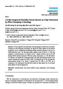
Global water challenge Fresh water is one of the earth’s most valuable resources. With an increasing global population and economic growth, our planet gets thirstier. Habitat is created in regions that don’t have sufficient precipitation, so the population and agriculture is often supported by water stemming from aquifers. However, these water sources can be over-exploited as well, and are thus limited. In some areas these aquifers, that have been filled over tens of thousands of years, are becoming increasingly depleted, and others have seen salinification due to an intrusion of ocean water [17] . Also the climatic change will influence the areas where a constant freshwater supply is available, and though the models vary, an increasing water scarcity similar to the projected one in Fig. 1.1 is likely.

Figure 1.1: Projected water scarcity in 2025 according to Seckler et al. [88] Economic water scarcity refers to regions that need to embark on massive water development programs to actually utilize their otherwise sufficient water resources. Therefore, humanity cannot solely rely on precipitation as source of fresh water, especially also because surface waters can easily be polluted and are thus often not safe for human consumption. The most abundant water source is undoubtedly sea water, and the recent decades have brought forward new technologies and vast improvements for seawater desalination techniques [24] . Yet, some of the desalination techniques only work economically when implemented at large scales, and all of them are bound to the vicinity of a water body. This means that transportation costs have to be considered for the economic and 3

Chapter 1. Introduction: Water from air energetic water price as well. For remote areas, this implies that the prices per m3 can increase significantly. Fortunately, our planet supplies us with a very sustainable form of water transport powered by solar energy: evaporation.

1.2

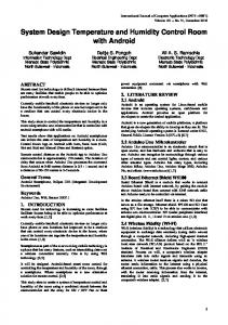
Atmospheric vapor as potential freshwater source The earth’s atmosphere contains approximately 13 000 km3 of (liquid) water in the form of water vapor. This corresponds to 3.7% of the earth’s total fresh water reserves [32] . Annually a net water vapor flux of 45 500 km3 is transported from the sea land-inwards [74] , and as the atmospheric temperature decreases with increasing heights, this also means that most of the water is close to the surface. The precipitation of this water vapor is the natural source of our fresh water. Yet, some areas lack the climatic and geographic conditions that lead to precipitation. In such cases, technology can fill this gap to make water readily available. Humidity harvesting or atmospheric water generation (AWG) describes this process of getting drinking water out of ambient air. Atmospheric air always contains a certain amount of water vapor, which stems from evaporation over water bodies or from terrestrial evaporation. The amount of water vapor therefore depends a lot on the regional conditions, as well as the temperature. The temperature is important as it determines the maximum concentration of water that can be present in the gas phase. This concentration, expressed by its partial pressure, is called the vapor saturation pressure. Heuristically speaking it can be said that when water molecules get close enough to each other, their attractive forces can lead to agglomeration of the individual molecules to form small liquid water bodies (= condensation). Yet, with increasing temperature, and thus increasing kinetic energy of the water molecules, the attractive forces are no longer sufficient for a net agglomeration and thus more water molecules can coexist in vapor phase. From these considerations it also follows that when a volume which contains water vapor is cooled down far enough, the point will be reached where the water starts condensing (= dew point). This is the underlying principle for the occurrence of rain and fog, which is also used for humidity harvesting. Some examples of applied humidity harvesting systems are presented in Fig. 1.2. The example that nature itself provides for extracting water from the atmosphere is the Namib Desert beetle [35] (Fig. 1.2a), which is imitated by mankind using fog nets [26] (Fig. 1.2b). The beetle stretches its body into a foggy breeze and due to its specialized surface the water is collected and runs 4

Atmospheric vapor as potential freshwater source

(a) Namib Desert beetle

(b) Fog nets

(c) Radiative cooling

(d) High mass cooling

(e) Active cooling (I)

(f ) Active cooling (II)

Figure 1.2: Various methods for water generation/collection, that make use of the water stored in the atmosphere. While the (a) Namib Desert beetle [97] and (b) fog nets [27] collect tiny liquid water droplets (fog), the other methods induce condensation of the water vapor by cooling. This can be provided by (c) radiative cooling [75] , (d) high masses that store the cold of the night [83] , active cooling via (e) a wind driven [21] or a (f ) diesel driven [42] heat pump.

to its mouth. Yet, this can only happen in areas, where the air already cools off far enough to get natural condensation (fog). In any other case the cooling has to be provided. For this purpose it is possible to make use of radiative cooling (by using very thin collection films) [14] as shown in (Fig. 1.2c), or to use the big heat storage capacity of high masses that have cooled down during the night [48] (Fig. 1.2d). Alternatively it is also possible to use active cooling, which means driving a heat pump by an external energy source. Among others, this source can either be wind power [21] (Fig. 1.2e) or a diesel generator [42] (Fig. 1.2f) which is already used in emergency water generators. Also electrically driven units are available to produce freshwater indoors (not shown) [91] . The wind driven humidity harvesting unit of “Dutch Rainmaker”[21] (Fig. 1.2e) serves as a reference system for this thesis. 5

Chapter 1. Introduction: Water from air

Energy requirements When ambient air is actively cooled down to condense water, a significant part of the enthalpy change can be attributed to the cooling of air, rather than the condensation process. Figure 1.3 shows the energy required for the cooling of one m3 of air (T = 30 ◦ C, relative humidity (r.h.) = 50%, absolute humidity (a.h) = 15 g/m3 ).

60 ta

to

50 Energy requirement (kJ)

1.3

ne le

y rg

40 ing

30

l coo

20

ing ens

con

air

or vap

d

10 0 30

cooling condensate

25

20 15 10 Temperature (°C)

5

2

Figure 1.3: Energy required for cooling one m3 of ambient air (T=30 ◦ C, r.h.=50%), and the contributions of the different processes. The main contributions are: • the latent heat of condensing the vapor ≈ 2260 J/g • the specific heat for cooling the air ≈ 1 J/g K • the specific heat for cooling vapor ≈ 2 J/g K • the specific heat for cooling the condensate ≈ 4 J/g K As water vapor only makes up a small fraction of the gases in atmospheric air, the condensation energy is not the major contribution, even though the latent heat of condensation is orders of magnitudes larger than the specific heat. The majority of the energy needs to be invested for the cooling of air. In the sample volume of air shown in Fig. 1.3, the air needs to be cooled down to the dew point of 18.5 ◦ C (investing 14 kJ) before condensation occurs. When it is cooled down further to 2 ◦ C to condense more water, only 42% of the energy is actually used 6

Concentrating the vapor for condensing and cooling the water while the remaining 58% are wasted on producing cold air.

1.4

Concentrating the vapor To avoid investing a lot of energy on the production of cold air, the water vapor can be concentrated prior to the cooling process. This facilitates a more efficient use of the energy for the desired condensation process. In literature two main processes are described for the vapor concentration: the use of desiccants (liquid [62] or solid [93] ) and the use of selective membranes [3] . Desiccants are materials low in vapor pressure that absorb the water vapor from an incoming air stream. Once the material is saturated it needs to undergo a regeneration step. This can either be achieved by cyclic operational conditions or in a spatially separated step. Desiccant methods have the advantage of being able to make use of the daily temperature fluctuations and to work almost passively, but this is borne by reduced water output due to the cyclic operational conditions. The use of spatially separated liquid desiccant dehumidification methods, on the other hand, is also very energy intensive as it requires additional energy for the regeneration, as well as for the condensation step. Yet, this technology, and how to design it more energy efficient is also matter of current research (especially for the use in air conditioning systems) [109] .

Membrane technology A water vapor selective membrane is a material that has a high permeability for water vapor, and a low permeability for other gases like N2 or CO2 . It can be used to separate the ambient air from a confined space in which the water vapor is concentrated and condensed. The driving force for the water permeation is the vapor pressure difference. As shown in Fig. 1.4 and according to Metz [64] , this driving force is maintained by a vacuum pump and a condenser that lowers the vapor pressure to the saturation pressure at the condenser temperature. The vacuum pump removes the non-condensable gases to keep the system pressure constant. In this way, the cooling power can be used very efficiently for cooling and condensing water vapor. Water quality

Besides an increased energy efficiency, a humidity harvesting

unit working with water vapor selective membranes has another major advantage over direct condensation from the air: an increased water quality. As the membrane is a dense layer that is highly selective to water vapor only, the permeation of bigger objects such as viruses or bacteria is virtually impossible. 7

Chapter 1. Introduction: Water from air

Figure 1.4: Conceptual water production system with water vapor selective membranes. The permeated water is thus ultra-pure and free of contaminants. With the proper maintenance of the water storage facilities this ultra-pure quality can be maintained. To make this safe water apt for drinking, minerals should be added before consumption. Yet, this is a fairly easy step as compared to post condensation treatment required in other technologies.

1.5

Current applications and framework for this thesis At the time this thesis started membrane assisted dehumidification had not received a lot of attention. Most publications that dealt with dehumidification were using expensive zeolite membranes [36,84] . Zeolite is a material with well defined pore sizes in the range of a few angstrom. As it can absorb a lot of water in its pores, it can not only be used as a very good desiccant, but also as a highly permeable membrane material (≈ 20 000 GPU i ). Yet, the selectivities that can be achieved are rather low (≈ 200 [107] ). Also polymeric membranes have already been tested in the dehumidification of compressed air [52,105] or natural gas [55] . These processes aim for the water removal in order to achieve a valuable retentate. In order to make the removed water itself the product, low cost membranes with high permeability and high selectivities are needed. The discovery and development of materials such R as mixed block polymers PEO-PBT [67] , Pebax 1074 [81] or SPEEK [56] made

polymeric membranes a suitable tool for dehumidification processes in which the recovery of the water is similarly important as the retentate quality. This has been demonstrated by a pilot scale system for flue gas dehydration [90] . Due to these promising results, an EU-FP7 Project called “CapWa”[18] started i

8

1 GPU (Gas Permeation Unit)≡ 3.3465 · 10−10 mol/s Pa m2

Thesis outline in the end of 2010 to investigate the use of novel membranes for the capturing of evaporated water in power plants. The main goal of that project was to optimize and scale up a smart membrane system (mainly tested with SPEEK and PEBAX), and to make an industrial scaled pilot from the laboratory setup. Based on the proven water vapor permeabilities and selectivities of polymeric membranes [19,67,81] , and the successful application in flue gas dehydration [90] , the scope of this thesis is to evaluate the usability of such water vapor selective membranes for the recovery of fresh water from the ambient air, at vapor pressures which are much lower (20–30 mbar) than those of flue gas (several 100 mbar). This means that: • the driving forces are lower, and the maintenance of the lower permeate side vapor pressure is more delicate; • the influence of leakages or permeation of other gases is a lot bigger compared to applications with higher driving forces; • the vapor transport from the membrane section towards the condenser needs to be ensured to achieve efficient condensation; • transportation resistances like concentration polarization have to be considered, as they decrease the membrane performance; • the energy required for the feed flow has to be evaluated with regard to achievable water permeation rates. These concerns as well as basic design questions need to be addressed in order to achieve valuable conclusions about the feasibility of such a humidity harvesting unit. The way these are being dealt with is described in the thesis outline.

1.6

Thesis outline In Chapter 2 the boundary conditions for membrane assisted humidity harvesting are defined. Various options for the different elements are considered and evaluated to result in a preliminary choice of components. This choice is evaluated theoretically in Chapter 3 by a permeate side system analysis. A model is developed that assesses the influence of atmospheric conditions, membrane characteristics, and leakages on the water production rate. A low pressure recirculated sweep stream is identified as the most energy efficient way of maintaining a high driving force while lowering the energy requirement for the vacuum generation. 9

Chapter 1. Introduction: Water from air This new process scheme is evaluated experimentally in Chapter 4. The limitations of sweep gas and vacuum as driving force are shown, and the possibility of increasing the permeation rate with a low pressure recirculated sweep stream is demonstrated. In Chapter 5 a feed side model, based on the kinetic theory of gases, is developed to predict the water vapor permeation rate for a given feed flow and partial pressure difference in hollow fiber membranes. With this model it is possible to relate a permeation rate to the energy required for driving the feed flow and thus to find the energetically most ideal fiber dimensions and flow speed. Chapter 6 combines the permeate side model of Chapter 3 and the feed side model of Chapter 5 to create an energetic analysis of membrane assisted humidity harvesting. Based on these results a recommendation for the design of a large scale humidity harvesting unit is given. To implement this large scale unit, some technological challenges have to be overcome. Chapter 7 describes two of the main challenges. These are a suitable membrane material/unit that shows the required permeabilities, and an immediate in-line measurement system to be able to predict the water production rates and to adapt to changing internal and external influences. The main findings of this thesis are summarized in Chapter 8.

10

2 Design considerations for humidity harvesting using water vapor selective membranes

11

Chapter 2. Design considerations Abstract In this chapter the main design questions for a humidity harvesting unit working with water vapor selective membranes are raised and evaluated. Based on the essential building blocks, the design of the most suitable membrane unit, the driving force for the permeation, the vapor transport towards the condenser as well as the condenser conditions are discussed. Different options for the water production are considered and evaluated for their aptness in humidity harvesting. This evaluation also includes an overview of available components in order to assess the practical feasibility. The chapter concludes with the recommendation of using hollow fiber membrane modules and a low pressure recirculated sweep stream to keep up the driving force and vapor transport towards the condenser.

12

Introduction

Introduction In Chapter 1 it has been shown how a humidity harvesting unit could profit from water vapor selective membranes. Yet, a system working with membranes requires a very different design and has other critical elements than a unit without. The only given necessities for such a system (shown in Fig. 2.1) are the membrane unit, with water vapor selective membranes, that separates the ambient feed side from the permeate side and a condenser to specifically cool and condense the water vapor. To keep the process running, the transport of water vapor across the membrane and towards the condenser needs to be maintained.

permeate side

membrane unit feed side

2.1

condenser vapor transport

membrane Figure 2.1: Basic elements for membrane assisted humidity harvesting.

Design questions From these fundamental tasks the following main design questions can be derived. • What is the most suitable membrane material and module layout to achieve high water vapor permeation? • How can the driving force for the water vapor permeation be imposed? • How should the system be arranged to assure vapor transport away from the membrane towards the condenser, in order to avoid local concentration buildup and thus a reduction of driving force? • How can the condenser contribute most effectively to maintaining the driving force for vapor permeation, and how much water can it produce? • What are the operational conditions that allow the most energy efficient humidity harvesting, and can it be advantageous over the conventional system? 13

Chapter 2. Design considerations

2.2 2.2.1

Possible choices of design and components Membrane unit The membrane unit is the centerpiece of this system. It comprises two main elements that need to be considered: the membrane material (permeability, selectivity) and the membrane module layout. Membrane material There are numerous materials which have been reported to have high permeability for water vapor, while being almost impermeable to other gases like nitrogen or carbon dioxide. These materials are, among others, commercial polymers like R [81] R [2] Pebax or Nafion , as well as experimental compounds like SPEEK [37] ,

PEO-PBT [65] or Poly-Dopamine [76] . Even graphene based membranes have been reported to show extremely high vapor permeance [70] . Yet, not only the material property of the permeance is relevant to the permeation rate, but also the thickness of the membrane layer through which the dissolved molecules have to diffuse [102] . Therefore, also the ability of the membrane material to form very thin skin layers of composite membranes [80] is of high relevance for the permeation performance. R As, apart from the extremely expensive Nafion membranes, we only know of

less suitable PDMS membranes [61] which are commercially available as membrane modules, the choice of the ideal membrane material is part of the ongoing research as will be described in Section 7.2. Finding the right membrane material, or even compositions of materials as used for thin film composite membranes (TFC) [47,110] , is of high priority as the permeance of the membrane module determines the required membrane area. This is a critical parameter concerning the cost effectiveness of membrane assisted humidity harvesting. The experiments are mostly performed with a SPEEK membrane that was made available to us R by Dr. Sijbesma from Parker Inc.

Membrane module layout The layout and structure of the membrane unit can have a big influence on the vapor permeation performance. The most common module types are plate and frame, spiral wound or hollow fiber membranes [49] (see Fig. 2.2). Even though the flat-sheet module types are supposedly more reliable, the hollow fiber membranes are not only cheaper [49] , but also have higher packing densities [4] . This is relevant as the desired water production rate is in the order of several cubic meters per day, which requires surface areas of several thousand m2 . The performance of a membrane module also depends on the operational 14

Possible choices of design and components

(a) Hollow fiber module

(b) Spiral wound membrane module

Figure 2.2: Different module types as shown by Baker [4] . (a) Hollow fiber membrane module with an inside-out configuration, and (b) the schematic flows in a spiral wound membrane module.

mode. In case of the hollow-fiber membrane modules, two distinguished flow patterns are common: flowing the feed through the inside of the fibers, collecting the permeate on the outside (inside-out) (see Fig. 2.2a), or the other way round (outside-in) [103] . The flow of the feed through the membrane module is important, as it not only determines the pressure loss and thus the work requirement, but the flow pattern also influences the local vapor distribution and therefore the efficiency of permeation. As boundary layer effects (e.g. concentration polarization), can play a dominant role in the resistance to vapor permeation [57] , this work focuses on the inside-out operational mode in hollow fiber membranes. Such a configuration provides a more controllable environment where boundary layer effects can be accounted for. Additionally the possibility of varying the dimensions of the fibers enables an effective (energetic and/or economic) use of the membrane area. Above all, they carry economical and design advantages. We will come back on these items in Chapter 5 and 6.

2.2.2

Vapor transport Permeation The driving force for the permeation across the membrane is the partial pressure difference. This can be generated by lowering the permeate side partial pressure or by pressurizing the feed flow and therefore also the upstream side partial pressure [50] . In humidity harvesting applications, the feed flow is taken from the ambient air. This means that the water vapor makes up only a small part of 15

Chapter 2. Design considerations the total gas composition (1–3%). Therefore, compression of the feed is very energy intensive and could even result in the unwanted condensation of the water vapor on the feed side. This can happen when, by compressing the air, the vapor pressure exceeds the saturation pressure. Thus, lowering the downstream side vapor pressure is energetically preferential for this application. The most commonly reported methods for achieving this are: • lowering the permeate side total pressure, which consequently also results in a reduction of the partial pressures [51] ; • introducing a sweep stream which has lower vapor content than the feed [67] ; • combining both methods to create a low pressure sweep stream [99] ; • selective removal of the vapor content by means of e.g. condensation [92] . Permeate side vapor transport Another aspect to maintaining a high driving force, is the water vapor transport away from the membrane interface towards the condenser. This avoids a local partial pressure buildup that hinders permeation. Eventually the condenser acts as a sink for water vapor, as it reduces the vapor pressure to the value of the saturation pressure at the cooling temperature. However, this only sets the vapor pressure at the condenser surface and not directly at the membrane interface, which is the relevant parameter determining the vapor permeation rate. Thus, the transport towards the condenser needs to be facilitated as well. This transportation can be driven by diffusion and convection. Diffusive transport

According to Fick’s law, the diffusive flux is proportional

to the diffusion coefficient and the concentration gradient of a specific species. The diffusion coefficient is pressure dependent [60] , and therefore the diffusive transportation of water vapor towards the condenser can be increased by reducing the permeate side pressure as well as by reducing the distance between the condenser and the membranes. A possible setup configuration, making use of this diffusive transport and a condenser to maintain a constant driving force across the membrane, can look similar to the configuration shown in Fig. 2.3. In this arrangement the housing of the membrane module is cooled, and thus pathways are as short as possible. Additionally a vacuum pump can be used to lower the permeate side pressure to increase the diffusive transport further. However, such configurations are not commercially available and would obviously require delicate and expensive construction work, as cooled surfaces 16

Possible choices of design and components

Figure 2.3: Possible design of membrane assisted humidity harvesting with diffusion driven vapor transport towards the condenser. The vacuum pump can be used to increase the diffusion coefficient.

need to be provided in close vicinity of only a few membrane fibers (too many fibers can again result in a local concentration buildup in the inter-fiber space). Additionally the controllability and maintenance of such a system would be difficult, as the different unit-cells are not that easily reached when only a few fibers are embedded in a cooled housing. The space required for the necessary membrane and condensation area would increase substantially as well. Therefore, diffusion as main driving force can be discarded for our application. Convective transport

The other way to facilitate water vapor transport

towards the condenser is via a convective flow. This means that the movement of the individual molecules is part of a bulk flow. This bulk flow can either be created by the use of a sweep stream or by lowering the total permeate side pressure with a vacuum pump. In the latter case, any permeating gases (that increase the local pressure) follow the pressure gradient imposed by the vacuum pump. The big advantage of a higher convective flow is that it allows for a modular construction of the humidity harvesting unit. Standardized membrane units, condensers and pumps can be used and connected in line of the convective flow. This makes it possible to use commercially available products and eases the construction. Additionally the maintenance is more simple as the different components can be accessed individually. On the other hand, an imposed convective flow like the sweep stream also needs more energy for the cooling process, as the heat requirement is proportional to the mass-flow. The different operational modes and their possible combinations are therefore 17

Chapter 2. Design considerations evaluated theoretically (Chapter 3) and experimentally (Chapter 4) in this thesis. The energetically most efficient option that follows from this analysis is to create a convective flow by recirculating air from the condenser outlet at a reduced permeate side pressure, as sketched in Fig. 2.4.

feed

membrane unit

external sweep flow

buffer tank retentate

water

Figure 2.4: Possible design of membrane assisted humidity harvesting with an induced convection via an external or a recirculated sweep flow generated by a pump. The total pressure can be controlled by a vacuum pump (right).

2.2.3

Condensation The condenser has the essential function of collecting the water, and limiting the vapor pressure on the permeate side. For the latter, a very low condenser temperature is favorable, to lower the saturation pressure as far as possible (compare Fig. 2.5) in order to achieve the maximum driving force across the membrane. Yet, apart from requiring more energy for cooling the convective stream, freezing is another disadvantage of temperatures chosen too low. When the condenser temperature is set below the freezing point, then additional energy is required for the latent heat of the phase change. Even though some of this energy could be reused, an ice-layer considerably impairs the heat transfer rate. Therefore condenser temperatures above the freezing point are advisable. Due to the temperature dependent increase of the vapor saturation pressure (see Fig. 2.5) the temperature should therefore be close to the freezing point. This is the reason, why in this work we focus on a cooling temperature of 2 ◦ C (≡ 7 mbar vapor saturation pressure). 18

Possible choices of design and components

vapor saturation pressure (mbar)

45 40 35 30 25 20 15 10 5 0 −5

0

5

10 15 20 temperature (°C)

25

30

Figure 2.5: Water vapor saturation pressure as function of the temperature according to the Magnus formula [104] . Various methods of industrial cooling are available for such temperatures. Of these the compression cooling cycle (using ammonia) seems to be the most appealing option. Other options like e.g. Vortex tubes (requiring pressurized air) [25] or thermoelectric cooling (requiring electricity, and lower efficiency) [38] are less relevant alternatives as they are more energy intensive. The fact that the condensation process occurs under low pressure conditions might raise concerns about the absence of nucleation particles. Yet, condensation in vacuum is already successfully implemented in applications such as pervaporation [43] or vacuum distillation [16] . Therefore, such condensers could also be suitable choices for the application in vapor permeation.

2.2.4

Support components According to the preceding discussion, an induced convective flow is desirable for the vapor transport towards the condenser. As mentioned, this can be realized using either a vacuum pump, a sweep stream or, ideally, a combination of both. Vacuumpump A vacuum pump can be used to lower the total permeate side pressure. This brings about a number of advantages for the vapor transport: • it reduces the permeate side vapor pressure to maintain the driving force; • it creates a convective flow towards the condenser and vacuum pump; • it increases the diffusion coefficient to reduce boundary layer effects [57] . 19

Chapter 2. Design considerations Due to the considerations about the condenser the end vacuum does not need to be below 7 mbar, which is usually considered as rough to medium vacuum. Such a vacuum can be achieved with a number of vacuum pumps but, due to the relatively high vapor contents, oil sealed pumps like the rotary vane pump should be avoided. Depending on to the final operational pressure, this leaves a choice of e.g. liquid ring pumps, scroll pumps, screw pump or roots pumps. According to the desired dimension of the humidity harvesting unit (compare Chapter 6), the vacuum pump needs to displace gases in the range of 600 m3 /hr. These values are best achievable with industrial root pumps that also work with a gas-ballast to increase their water vapor tolerance [78] (e.g. Pfeiffer Vacuum LRS 3 [79] or ACG 600 [77] ), or a combination of a few smaller pumps (e.g. 4 Leyvac LV 140C screw pumps ` a 145 m3 /hr [73] ). The ultimate pumping requirement is subject to the membrane material used and the leak-tightness of the module fabrication. Yet, these pumps show that the system requirements are in the same range as the available products, and that even further up-scaling would be possible (available pumps have been found up to 1800 m3 /hr).

Recirculation pump To create a sweep stream with sufficiently high flow speeds but with low mass flow (to keep the energy requirement for the cooling as low as possible), recirculation of the air from the condenser outlet at low pressures appears to be the energetically most effective solution (see Chapter 3). To create such a low pressure recirculated sweep stream as sketched in Fig. 2.4, a recirculation pump is needed. The main task of such a device is to displace relatively large volumes at low pressures against a small pressure difference. Ideally this could be a hermetically sealed fan. Due to the low pressure buildup in axial fans [96] , as compared to e.g. centrifugal fans, this fan type is preferable. Even though the capacities of axial fans are smaller than those of centrifugal fans, they can be sufficiently high for the required recirculation stream [95] . Unfortunately no potential supplier for such hermetically sealed fans working at low pressures could be found yet, even though they are crucial for the large scale implementation of a humidity harvesting unit working with membranes (see also Chapter 7). For the proof of principle in this thesis a vacuum pump is chosen to recirculate an air stream back to the membrane module. Even though this is energetically not recommendable, it is an hermetically sealed pump that avoids leakages in the system, while still being capable of providing the desired flow-rates. 20

Preliminary choice of components Energy supply To drive the whole process an energy source is needed. The existing Dutch Rainmaker unit [21] is working with a windmill that mechanically drives the compressor of the ammonia cooling cycle and additionally powers a small generator for the electrical energy demand. However, for the process itself, the source of energy is irrelevant. Mechanical energy to directly drive the compressor of a cooling cycle is beneficial as it improves the efficiency. For this research however, it does not matter whether this mechanical energy is provided by a wind or water turbine, a diesel engine or even an electrical motor. To fully utilize the benefit of a humidity harvesting unit for drinking water production though, it is advantageous to be independent of existing infrastructure, which would favor a wind or solar driven energy supply.

2.3

Preliminary choice of components The above considerations lead to a preliminary choice of components and operational conditions which shall serve as a basis for the in depth analysis of the following chapters. The humidity harvesting system is therefore composed of the following constituents/conditions: • a hollow fiber module is used as membrane section to avoid/account for concentration polarization and to achieve higher packing densities; • the membrane material used for the experimental research is SPEEK due to it’s good permeation and separation properties. At the same time other materials are still investigated for their suitability for humidity harvesting; • to make use of commercially available state of the art technology the different components of the humidity harvesting unit are connected in a modular way; • a low pressure recirculated sweep stream is used to facilitate a convective vapor transport through the system components; • a condenser temperature of 2 ◦ C is used to produce high driving forces without running into the danger of freezing; • the system pressure is set below 100 mbar to avoid wasting energy on the cooling of the sweep stream.

21

3 System analysis of membrane facilitated water generation from air humidity

recirculation pump

H2O n.c. dried air

water vapor selective membrane

humid ambient air

low pressure section

vacuum pump

n.c. …non-condensable gases

23

Chapter 3. System analysis Abstract The use of water vapor selective membranes can reduce the energy requirement for extracting water out of humid air by more than 50%. We performed a system analysis of a proposed unit, that uses membranes to separate water vapor from other atmospheric gases. This concentrated vapor can then be condensed specifically, rather than cooling the whole body of air. The driving force for the membrane permeation is maintained with a condenser and a vacuum pump. The pump regulates the total permeate side pressure by removing noncondensable gases that leak into the system. We show that by introducing a low-pressure, recirculated, sweep stream, the total permeate side pressure can be increased without impairing the water vapor permeation. This measure allows energy efficiency even in the presence of leakages, as it significantly lowers the power requirements of the vacuum pump. A such constructed atmospheric water generator with a constant power of 62 kW could produce 9.19 m3/day of water (162 kWh/m3 ) as compared to 4.45 m3/day (334 kWh/m3 ) that can be condensed without membranes. Due to the physical barrier the membrane imposes, fresh water generated in this manner is also cleaner and of higher quality than water condensed directly out of the air.

This chapter is based on: Bergmair, D., Metz, S. J., de Lange, H. C. and van Steenhoven, A. A., “System analysis of membrane facilitated water generation from air humidity”, Desalination, 339, 26-33, 2014

24

Introduction

3.1

Introduction The increasing water scarcity, due to ongoing desertification, salinization of fresh water sources and a still increasing global population poses a major challenge for society. Access to safe drinking water is so substantial that it was made one of the United Nations “Millennium Development Goals”. Most approaches for generating new sources of fresh water focus on desalination techniques to make use of the seemingly unlimited water body of the oceans [22,28] . Another possibility, which has found less application up to now, is the extraction of water from the air humidity. The amount of water that can be present as vapor strongly depends on the temperature. Therefore, when a body of air is cooled down far enough, it will result in the condensation of the excess vapor which can then be collected. This cooling can either occur naturally (dew collection [14,71] ) or it can be achieved by investing energy [100] . Due to the relatively high latent heat of water, the energy requirements to condense water are usually orders of magnitude larger than the energy required for water purification methods. Thus, atmospheric water vapor processing can only be remunerative in the presence of natural or existing heat sinks (radiative cooling [29,72] , deep sea water [30,82] , otherwise unused heat-sinks [33] ) or in remote areas where the energy balance changes significantly when transportation is taken into account. In such locations a humidity harvesting unit may be driven by renewable energy, like solar [5,23,87] or wind [101] energy, so it could be a stand-alone application, independent of existing infrastructure. Besides the energy required for the condensation, a significant part of the energy demand in humidity harvesting is needed for cooling the body of air in which the water vapor is embedded at atmospheric conditions. If a cubic meter of air of 30 ◦ C with a relative humidity of 50% is cooled down to 2 ◦ C, only 43.6% of the cooling power is used for condensing water (9.66 g), while the remaining 56.4% is almost entirely spent on cooling air. A way to circumvent this sensible heat requirement is to concentrate the water vapor by the use of desiccants [1,34,45] . However, even with the recent discovery of advanced desiccant materials [108] the main disadvantage of this process is that a desiccant system works in cycles, reducing the maximum water output as a continuous process is not possible. Another method that brings about the same advantages, but allows for a continuous process is the use of water vapor selective membranes to separate the water vapor from the other gases prior to the cooling process [6] . The driving force for the permeation is the partial pressure difference across the membrane. This force is maintained with a condenser and a vacuum pump 25

Chapter 3. System analysis that displaces the inflow of non-condensable gases. Due to the use of a dense polymer membrane that is highly selective for water vapor, no pollutants or pathogens can pass the membrane, making the condensed water very pure. Also the membrane maintenance should not pose a major challenge as only air and vapor (therefore no scaling) is used as a feed and the absence of sunlight and aqueous environment do not favor bacterial or algae growth, which pose the greatest challenges to other common membrane technologies. In this paper we analyze the effects of operational and meteorological conditions (like temperature, humidity, permeate side pressure or water vapor pressure) on the water production and the energy efficiency of a system working with membrane separation. According to these and the membrane characteristics, such as permeability and selectivity, we suggest a system design and provide operational parameters, that can be used to significantly reduce the energy demand for the production of potable water.

3.2

Humidity harvesting with membranes To extract humidity from the air with the use of water vapor selective membranes we propose an installation that is schematically depicted in Fig. 3.1. A membrane module (I) exposed to a humid air stream (feed stream) is the centerpiece of that system. Due to its selective properties and an imposed driving force water vapor permeates through the membrane and the remaining dried air stream is discharged (retentate). The driving force for the water vapor transport over the membrane is maintained by two main components: a vacuum pump (II) that controls the total pressure on the permeate side and a heat pump that cools down and condenses the permeated water vapor at the condenser (III). Thus the water vapor pressure on the permeate side depends on the condenser temperature and the according water vapor saturation pressure. The condensed water is collected in the water collection tank (IV) from which the water can be pumped out. A buffer tank (V) can be added to increase the permeate side volume making the system less susceptible to pressure changes. A recirculation pump (VI) is used to create a low-pressure recirculation sweep stream. This facilitates the uncoupling of the permeate side water vapor pressure from the total permeate side pressure as will be described later on. 26

Humidity harvesting with membranes

feed stream

condenser (III)

water collection tank (IV)

membrane module (I)

retentate

buffer tank (V)

recirculation pump (VI)

vacuum pump (II)

Figure 3.1: Schematic representation of the membrane unit and the permeate side constituents of a humidity harvesting unit, working with water vapor selective membranes.

System parts and analysis 3.2.1

The membrane unit A water vapor selective membrane is a material that has a permeability for water vapor much larger than that for any other gas. While gas separation membranes are often porous structures with pore sizes small enough to separate molecules due to their different free path lengths (Knudsen Diffusion) [69] , membranes for vapor permeation and pervaporation can make use of the polarity of the water molecule. Such membranes are dense, thin films (polymers) which, according to the solutiondiffusion model [102] , have a high solubility for water (hydrophilic material) and a fast diffusive transport from one side to the other. Therefore, water vapor R [81] selective materials, like Pebax or PEO-PBT, can achieve permeances for

water vapor (PH2 O ) much higher than for other gases (Pi ), such as nitrogen (PH2 O/PN2 > 40000 [67] ), while maintaining a high permeability as well. To our knowledge the highest reported water vapor permeance has been achieved with an ultra-thin poly-dopamine layer, where a permeance of up to 3 · 10−6 mol/s Pa m2 (≡ 9000 GPU) was measured [76] . The driving force for permeation is the chemical potential difference, which, under given circumstances, is equivalent to the partial pressure difference between the feed and the permeate side of the membrane [102] . The permeation of a species 27

Chapter 3. System analysis i is described by: N˙ i = A Pi ∆pi

(3.1)

with N˙ i being the molar flow rate of species i, A the membrane surface area, Pi the permeance of the membrane towards species i, and ∆pi the partial pressure difference of this species across the membrane. As the vapor pressure in the feed stream cannot be modified (as function of temperature and relative humidity), the partial pressure difference for water vapor permeation can be induced by either reducing the total permeate side pressure, or by introducing a sweep stream that is dryer (thus lower water vapor pressure) than the feed. The physical barrier that the dense polymer membrane imposes also prevents particles and micro-organisms from passing to the permeate side and polluting the condensed water, which in turn is very pure and clean. The feed side of the membrane that is exposed to a (pre-filtered) air stream also lacks the aqueous surrounding, nutrients, sunlight and other factors that favor bio-fouling. Therefore, it can be expected that the permeation performance will not alter too much over time, as has also been observed in long term experiments for water vapor removal from flue gases [90] . Nevertheless the demand for membrane cleaning has to be assessed in actual field tests.

3.2.2

Non-condensables and leakage flow Equation 3.1 can be applied to every kind of gas, and thus an increased surface area increases the flow of non-condensable gases, such as nitrogen, oxygen or carbon dioxide, as well. The ratio of the permeances of two different species i and j defines the specific selectivity αij of a membrane: αij =

Pi Pj

(3.2)

The selectivities of a membrane for water vapor can be extremely high and thus the permeation of non condensables very low. Yet, there can also be different sources for non-condensable gases, like leakages in the membranes and the housing. The influence of these non-condensables in the system has 4 main consequences: - an increased vacuum pump performance is required to keep the permeate side pressure constant - the system needs increased cooling capacities for the sensible heat of the non-condensable gases 28

Humidity harvesting with membranes - an increased pumping performance increases the water vapor loss rate (see Eq. 3.3) + at a constant permeate side pressure, an increased presence of non-condensables leads to a decrease of the water vapor pressure and thus increases the driving force for water vapor permeation.

3.2.3

Condenser and vacuum pump In a hermetically sealed permeate-side section (with a perfect membrane and without leakage) the condenser works as a pressure regulator. The temperature of the cooled surfaces defines the saturation pressure of water vapor in the condenser element. Thus, at equilibrium, water vapor permeating through the membrane results in a condensation at the condenser as the additional vapor would exceed the saturation pressure of water, and the driving force remains a constant. To counteract the stream of non-condensable gases that get into a real system, a vacuum pump is needed to keep the pressure at the desired level. The required pump-rate of the vacuum pump is not only determined by the inflow of non-condensables, but also by the saturation vapor pressure (psat ) and the total pressure (ptot ) at the condenser, as the non-condensables need to be pumped out of a volume that contains a water vapor fraction of psat/ptot as well. The pump-rate of the vacuum pump (N˙ vp ), required to compensate for an inflow rate of non-condensables, N˙ nc , can therefore be written as i : N˙ vp = N˙ nc

ptot ptot − psat

(3.3)

where ptot is the absolute pressure set by the vacuum pump, and the difference between ptot and psat describes the partial pressure of non-condensables (pnc ). Eq. 3.3 shows that the closer the total pressure is to the saturation pressure, the more water vapor has to be pumped out together with the non-condensable gases to maintain a constant pressure (= vapor loss rate). This decreases the efficiency of the membrane unit, and increases the power requirement of the vacuum pump as more gases need to be displaced. Also the efficiency of a vacuum pump usually decreases with increasing water activity. A shift to higher operating pressures lowers the power requirement of the pump (see also Eq. 3.6). Due to the smaller pressure difference towards the atmospheric pressure also the leakage flow into the system is reduced (experiments indicate that leakage flow for a membrane module is a function of pressure, unlike i

For ptot > psat N˙ tot/N˙ H2 O , as the pump rate cannot exceed the inflow rate.

29

Chapter 3. System analysis a choked flow). Yet, a higher pressure also results in a lower driving force across the membrane and this reduces either the water output or increases the required membrane surface area.

3.2.4

Recirculation pump A way to overcome the reduction of the driving force when increasing the total permeate side pressure, is the use of a sweep stream. If the gas mixture at the outlet of the condenser (e.g. from the buffer volume) is pumped back into the system through the membrane section (compare Fig. 3.1) the total pressure of the system can be chosen freely, while the driving force will be determined by the sweep stream, and its water vapor pressure (equal to the saturation pressure at the condenser). The recirculation pump only has to displace the gas against a pressure difference caused by frictional resistance of the connective parts (compare Eq.3.9). This pressure buildup can be kept very low with the right dimensioning of the connection pieces. Working with a sweep stream at higher total pressures combines the advantages of reduced vacuum pump requirements and reduced vapor loss rate (compare Eq. 3.3 and 3.6). Furthermore, a forced convection on the permeate side has been reported to reduce the permeation resistance stemming from the membrane support [9,53] . However, the higher the pressure and the higher the flow rate, the more energy has to be used for the sensible heat of cooling the recirculated stream.

3.3

Model description The main process determining the water production rate, the power requirement and the equations used for their calculation are indicated in Fig. 3.2.

Membrane permeation The equations for the permeation of the different gases according to Eq. 3.1 are given by: N˙ H2 O, perm = PH2 O A (pH2 O, feed − pH2 O, perm )

(3.4)

PH 2 O N˙ N2 , perm = A (pN2 , feed − pN2 , perm ) αH2 O,N2

(3.5)

The model focuses on these two gases because of the extremely high permeance towards water vapor, and the abundance of nitrogen in the atmosphere. Other gases like CO2 are not considered separately, as their contribution to the inflow 30

Model description

membrane module

feed stream

retentate

permeation: Eq. 4 & 5 flow rate: Eq. 11 pressure loss in connections: Eq. 10

power recirculation pump: Eq. 9

buffer tank

power for condenser: Eq. 7 power vacuum pump: Eq. 3 & 6

water collection tank

Figure 3.2: Main processes that are used for the model with the references to the equations (of this chapter) used for solving it.

is marginal and can be included in the term for the leakage rate. These equations assume a uniform driving force throughout the whole membrane module. An in depth analysis would need to consider (partial-) pressure buildups [13] , depletion of the permeating substance along the membrane due to ongoing permeance [7] , as well as the influence of the concentration polarization [68] or the influence of the support layer [9] . All these factors can be summarized in the overall performance of the membrane module, and thus the standard value used for the permeance is 1.67 · 10−6 mol/s Pa m2 (5000 GPU) rather than the maximum measured by Pan et al. [76]

Vacuum pump The power requirement for the vacuum pump working at a displacement rate of N˙ vp is calculated as an isentropic compressor that transports gas from pressure p1 (operating pressure of the system) to a higher pressure p2 (1 atm), corrected with the isentropic efficiency, ηS . According to Bird et al. (1960) [10] (neglecting the change of kinetic energy):

Pvp

1 γRT = ηS γ − 1

"

p2 p1

 γ−1 γ

# −1

N˙ vp

(3.6) 31

Chapter 3. System analysis where γ is the ratio of specific heats (with a value of γ = 1.4), R is the gas constant with a value of R=8.314 J/mol K, and T is the ambient temperature in K. For small pumps the isentropic efficiency can have values between 0.6 and 0.7 [20] . To account for the general efficiency (frictional losses or the influence water vapor might have) a general efficiency of ηvp = 0.5 was used as conservative estimation for the calculations. In case of a vacuum pump which is more susceptible to water vapor, the previously mentioned buffer tank could be needed, as it allows the temperature of the gases to heat up to the ambient temperature, and thus lowers the activity of the water vapor (as the saturation pressure - in contrast to the overall pressure - is not a linear function of temperature). This can be necessary to prevent condensation and therefore a decrease in energy efficiency of the pump.

Condenser The power requirement for the condenser is determined by the enthalpy change due to cooling and condensation of the in-flowing gas mixture: Pcond =

N˙ ∆H COP

(3.7)

where Pcond is the mechanical power required to cool and condense an incoming gas mixture with a flow rate of N˙ , ∆H is the difference in molar enthalpy at the inlet and outlet of the condenser (implemented by Junglas et al. (2008) [44] ), and COP is the coefficient of performance of the cooler. The reference COP used in these simulations is chosen according to the humidity harvesting unit of “Dutch Rainmaker”[21] which works (without membranes and at a temperature of about 30 ◦ C) at a COP of approx. 5 (oral communication with Dutch Rainmaker). Although the COP is a function of temperatures that increases with decreasing ambient temperature, the actual cooling efficiency of a system increases less than the ideal Carnot efficiency. It is mainly determined by factors outside the design of the cooling equipment and therefore less influenced by small temperature changes [106] . Thus the value is taken as a constant, and the potential increase of water output (which would be more pronounced in a system working with membranes) is neglected.

Recirculation pump The work requirement of the recirculation pump is calculated from the volume flow that needs to be displaced, and the frictional pressure buildup (∆p) caused by this volume flow (compare Eq. 3.9). For simulations with a recirculation flow, 32

Model description the connective parts were varied in dimensions to keep the frictional losses at a minimum. Therefore the power requirement of the recirculation pump, Prp , to create a volume flow, V˙ , can be approximated by the power requirement of a mechanical fan [20] : Prp = V˙ ∆p

(3.8)

Pressure loss in piping The connective parts between the elements are approximated as circular pipes. Their dimensioning is used to estimate the pressure buildup due to frictional losses in the flow. Too small dimensioning of the connective pieces can lead to a pressure buildup that results in a significant reduction of the driving force in the membrane unit. The pressure buildup can be approximated by the isothermal Bernoulli equation for ideal gases with the Darcy friction factor [10] . In terms of molar flow rates this can be expressed as:  − ln

p2 p1




p2 2 − p1 2 R4 π 2 l + + f =0 2 ˙ ¯ R 2N M RT

(3.9)

with p1 and p2 the inlet and outlet pressure, R the pipe radius, N˙ the molar ¯ the gas constant, T the absolute temperature, l the length flow rate of the gas, R of the pipe and M the molar mass of the gas mixture. f is the Darcy friction factor that is approximated by f = 0.0791/Re0.25 for turbulent flow. The Reynolds’ number was determined according to pipe flow where the (pressure dependent) density and viscosity were approximated by linear combinations of dry air and vapor.

Numerical solutions The system of equations describing the individual components and their interactions are solved using the numerical solvers of Matlab 2012b. The conservation of mass, N˙ tot =

X

N˙ i = N˙ permeation + N˙ recirculation + N˙ leakage (3.10) P Dalton’s law of partial pressures (ptot = pi ) and a restriction to physically relevant results, are taken as boundary conditions for the solvers. To investigate the influence of the individual parameters, calculations were performed, varying the desired parameter in a certain range, while all other parameters were kept constant according to Table 3.1, unless noted differently. These sample values were chosen according to realistic membrane characteristics and the membrane area such that the water output is approx. 18 m3/day. The 33

Chapter 3. System analysis Table 3.1: Model input parameters that will be varied around these given characteristic values input parameter membrane area permeability selectivity leakage flow ambient temp water vaporpressure feed condenser temp pressurevacuumpump ηvp recirculated vol. flow COP

value 2200 5000 36000 0 30 42 2 10 0.5 0 5

unit m2 GPU mol/s ◦C mbar ◦C mbar m3/s -

diameter of the connectors need to be adjusted for simulations with higher flow rates to avoid significant pressure buildup. These characteristic input parameters result in a daily water production of 18.03 m3/day at a constant mechanical power requirement of 107.7 kW (143.4 kWh/m3 ) of which 1.31 kW are consumed by the vacuum pump. The reference case does not include the recirculation pump which will be shown further on. The total energy requirement is composed of the work of the pumps and the heat of the cooling/condensation process (considering the respective COP ): Ptot = Pvp + Prp + Pcond

3.4 3.4.1

(3.11)

System analysis and influence of operational conditions Atmospheric conditions To evaluate the effect of atmospheric conditions (temperature and relative humidity), a humidity harvesting unit, capable of delivering 100 kW of mechanical energy which works at a COP of 5 is assumed. The amount of water that can be produced per day (and thus the energy efficiency) is calculated for different temperatures and relative humidities of the feed flow (shown in Fig. 3.3). It can be seen that for the model of a unit without membranes (H), an increasing vapor content in the air (higher relative humidity, or higher temperature), the water production increases, as the energy can be used more efficiently on vapor condensation. For a unit working with membranes (◦) on the other hand, the possible water output is almost independent of the temperature, as long as the water vapor pressure (driving force) is above a certain threshold. 34

System analysis and influence of operational conditions

16

75%

water production (m3/day)

%

100

14

%

50

25%

%

35

12 10

100%

8

75%

6

50% 35%

4

25%

2 0

10

15

20 25 30 35 atmospheric temperature (°C)

40

Figure 3.3: Daily water output for a 100 kW unit at different temperatures and relative humidities without (H) and with (◦) a membrane unit. The percentages indicate the relative humidities of the feed stream.

This can be explained by the high selectivity of the membranes. The amount of co-permeating non-condensable gases is relatively low, and therefore a lower water content in the air (which also results in a lower driving force), has the main consequence that more membrane area is needed to achieve a certain permeation rate. Only when the required membrane area rises to very high values (compare Fig. 3.4), the inflow of non-condensables starts to get influential and the energy required for cooling and pumping out these gases reduces the maximum achievable water output. Fig. 3.4 shows the water output of the data points of Fig. 3.3 plotted as a function of their water vapor pressure (right ordinate, ◦), and the membrane area required to permit such an output (left ordinate, •). The above mentioned dependence of the required surface area on the vapor pressure, and thus also the water production, can be seen and is especially pronounced for low vapor pressures. In fact in such an approximation, the amount of water that permeates through 1000 m2 of membrane area increases linearly with the partial pressure in the feed (0.26 m3/day mbar). This means that for the constant water output of 16.75 m3/day 3.26% more surface area is needed if the feed side vapor pressure drops by 1 mbar (see also Eq. A.1).

3.4.2

Membrane characteristics To see the influence of the membrane characteristics like area, permeability and selectivity and to investigate which of the factors previously described is 35

16

17

14

16

12

15

10

14

8

13

6

12

4

11

2

10

0

10

20

30 40 50 60 vapor pressure (mbar)

70

water production (m3/day)

required membrane area (1000 m2)

Chapter 3. System analysis

9 80

Figure 3.4: Membrane area (•) required for the water output (◦) as a function of the water vapor pressure in the feed at a constant power of 100 kW dominant for the water vapor transport, the water production has been calculated at constant membrane area as shown in Fig. 3.5, and at constant (high) selectivity (showing the linear relationship of Eq. 3.1 in Fig. A.1).

10 mbar

15

20 mbar

3

water production (m /day)

20

10 30 mbar 5 40 mbar

0

1000

2000

3000 selectivity

4000

5000

Figure 3.5: Influence of selectivity and total permeate side pressure on the water production with constant membrane area Fig. 3.5 shows that for a total permeate side pressure of 10 mbar, a lower selectivity and thus a higher flow of non-condensables results in a water vapor loss rate that exceeds the additional influx caused by the higher partial pressure difference. Therefore, the daily water output decreases with decreasing selectivity. For 20 mbar no effect seems to be dominant, and at higher pressures the decrease 36

System analysis and influence of operational conditions of water vapor pressure on the permeate side (due to the dilution of the water vapor with non condensable gases at constant total permeate side pressure) is dominant and the daily water output increases with decreasing selectivity. This increase in water output is accompanied by an increased specific mechanical energy requirement per unit mass of condensed water (Especif ic =

Ptot/m ˙ ).

Fig. 3.6 shows that for all pressures this specific energy requirement is increased with a decreasing selectivity. The comparatively high values for 40 mbar are

spec. mech. energy (kJ/kg)

750

700

650

600

30 550

0

20

mb

mb ar

ar

2000

4000 6000 selectivity

40 mbar 10 mbar

8000

10000

Figure 3.6: Specific mechanical energy requirement to produce one kg of liquid water for different selectivities at different permeate side pressures. caused by the low driving force for water vapor permeation at an almost unchanged driving force for non-condensables. This results in a higher sensible heat requirement for the cooling of these gases. The values for 10 mbar are mostly influenced by the high vapor loss rate and therefore the energy wasted on cooling and pumping out bigger amounts of gas and vapor (also against the largest pressure difference). This effect is decreasing with increasing selectivity in accordance with Eq. 3.3. For 20 and 30 mbar the vapor loss rate is lower, and thus the relative contribution of the sensible heat is smaller as also more water condenses. A low selectivity mainly increases the power requirement for the vacuum pump as more gases need to be displaced. For large enough selectivities, the sensible heat for cooling the air contributes only little to the total power demand due to the latent heat of condensation being much larger than the specific heat of air (for αH2 O,N2 > 100 the contribution is less than 1%). Fig. 3.6 shows that the curve for the energy requirement flattens out towards higher selectivities. Therefore, although the membrane material with the highest 37

Chapter 3. System analysis

spec. mech. energy (kJ/kg)

690 10 mol/s

680 670 660

90 mol/s 650 70 mol/s 640 50 mol/s 630 30 mol/s 620 40

60

80 100 pressure (mbar)

120

140

Figure 3.7: Mechanical energy requirement for different recirculation streams (10 - 90 mol/s) and permeate side pressures when a leakage flow of 0.5 mol/s is given possible selectivity is desirable, the energy gain will not be significant anymore for membranes better than the present day ones.

3.4.3

Recirculated sweep stream at low pressures In a system at higher pressures and without leakages, a dry-gas sweep stream increases the driving force for water vapor permeation, and therefore also the water production. However, it also increases the sensible heat required for cooling the recirculated gases. Therefore the specific energy for the water production increases almost linearly with the recirculation stream (for an example of 100 mbar see Fig. A.3). In a system with a non-negligible inflow of non-condensables the linear trend described above will change and working at higher pressures can even become the more energy efficient option, as it unloads the vacuum pump. The most energy efficient operational parameters are now non-trivial combinations of system pressure and recirculation flow. Figure 3.7 shows a system with a leakage flow of 0.5

mol/s

(as a comparison: the total water permeation flow is estimated

to be around 11 mol/s), where the relative work requirement has been plotted against the operation pressure for various recirculation speeds. The following observations can be made: • A recirculation stream that is too small only increases the work requirement for the recirculation and the sensible heat without significantly increasing the water output. Thus the relative work per unit mass of condensed water is increased. 38

System analysis and influence of operational conditions • A sufficiently large recirculation flow decreases the permeate side vapor pressure to an extent that the increased water output exceeds the additional energy demand. This therefore lowers the relative work per unit mass of water produced. • Above a certain threshold, the water output is not further increased, but the relative energy requirement increases due to the additional sensible heat requirements of the superfluous stream. According to this graph, the minimal relative work is found at operational conditions of 80 mbar and a recirculation flow of 30 mol/s. In the same way, the optimal operation pressures are determined for different leakage flows and plotted against the recirculation speed, as can be seen in Fig. 3.8.

spec. mech. energy (kJ/kg)

800

1.5 mol/s; 180 mbar 750

bar

1 mol/s; 120 m 700

0.5 mol/s; 80

mbar

650 0 mol/s;

600

40 mbar

550 20

40 60 80 recirculation flow (mol/s)

100

120

Figure 3.8: Specific mechanical energy requirement for various recirculation speeds and leakage flow rates shown for the pressures at which the minimal values could be achieved An increasing leakage flow, increases the specific energy for the water production, and also raises the system pressure needed to achieve this minimal specific energy (to reduce the power demand of the vacuum pump). At higher pressures the recirculation flow needs to be increased to decrease the partial pressure on the permeate side sufficiently, shifting the energetic minima to increased flow rates. Above these values the sensible heat requirement to cool the recirculated stream exceeds the additional water gain and increases the specific energy demand for all pressures alike. Despite higher energy costs, the water output of a unit with given membrane area can still be increased when increasing the recirculation flow (as shown for a 2200 m2 unit in Fig. 3.9), making the use of the membrane area more efficient. 39

Chapter 3. System analysis

water production (m3/day)

18 16

bar

0

/s; mol

40 m

ar

0 mb

l/s; 8 5 mo

0.

14

bar bar 0m 80 m 2 1 ; l/s; 1 o s / m l o 1.5 1m

12 10 8 6 4 20

40 60 80 reicrulation flow (mol/s)

100

120

Figure 3.9: Maximum water production for a given membrane area, for various recirculation speeds and leakage flow rates When driving the recirculation flow to a higher water output, the additional sensible heat requirement could partially be recovered by a heat exchanger. This option is considered in detail in Section A.3 (Appendix A). The results show that for a heat recovery of 50% the heat exchanger also contributes significantly to the frictional losses in the system. Additional power is required to drive the recirculation speed and the overall estimated energy gain is therefore only in the range of 1.9% compared to a system without the heat exchanger. Therefore, this option will not be further considered here, due to its limited gain. The presence of a recirculation stream also enables the adaptation to changing conditions. In case of symptoms of aging (e.g. membranes get brittle, show a deterioration of the selectivity, get holes, show reduced permeability) the leakage rate would change, and therefore also the required volume displacement of the vacuum pump. This change could be measured and the system pressure and recirculation speed adapted to match the altered circumstances (similarly to Fig. 3.8 and 3.9). Therefore energy losses can be kept at a minimum.

3.5

Example of a specific application The applicability of a humidity harvesting unit working with membranes is most suited for warm areas with high water vapor pressures but which have a lack of rain and no access to seas, lakes or rivers. The Negev Desert in Israel holds such places like e.g. Beersheba. In summer there is absolutely no precipitation, yet the average dew point is 16.3 ◦ C and the average temperature is 26.3 ◦ C [12] . A humidity harvesting unit in such an area could be enhanced a lot by the 40

Conclusions use of water vapor selective membranes. If one assumes a condenser temperature of 2 ◦ C, a membrane surface area of 5000 m2 , and a leakage flow of 0.1 mol/s (corresponding to a leakage rate of about 10−4 mbar l/s that makes up less than 2% of the total permeation), then the energetically ideal working conditions would be at a system pressure of 25 mbar, and a recirculation flow of 16 mol/s (equivalent to 16 m3/s). Under such conditions 9.19 m3 of fresh water could be produced per day, at a constant power supply of 62 kW (162 kWh/m3 ). 87.4% of this power is used for the condensation of water vapor only, indicating the high degree of efficiency. The water vapor loss rate is below 1%. Due to the leakage rate, however, a relatively high part of the total power has to be used for the vacuum pump (5.4 kW). Nonetheless the energy savings are significant. With a unit of equal power delivery, a conventional system (without membranes) cooling down the air to the same temperature would produce less than half the amount of water (4.45 m3 ), in which case only 43% of the energy would be used for the actual condensation process. This is also in accordance with other atmospheric water vapor processing systems, where the energy demand is reported to be between 270 and 500 kWh/m3 which would be the equivalent of 3 − 5.5 m3/day

[23] .

The same optimization could

be done for any given atmospheric conditions. As shown in Fig. 3.3 the efficiency of the system is mainly determined by the leakage rate (for given selectivities) and thus different locations with different temperatures and humidities would achieve similar values, yet, at the cost of more membrane area which is required to achieve the same water output as was discussed in reference to Fig. 3.4.

3.6

Conclusions In this chapter we have shown that the energy gain, when using membrane technology in humidity harvesting, is significant. The effect of membrane characteristics, temperature, humidity and leakage flows resembling realistic conditions have been evaluated. We have shown that when there is an inflow of non-condensable gases into the system, the energy balance can be improved significantly by non-trivial combinations of system pressure and a low-pressure recirculated sweep stream. It has been demonstrated that for a given input power twice the amount of freshwater can be produced with membranes, which is of superior quality. We expect that this enhancement can have a large impact on technologies using atmospheric water vapor as source of drinking water and can be a large benefit, especially for remote areas. Future research is focused on experimental evaluation of the model results. 41

4 Experimental assessment of a low pressure recirculated sweep stream

H2 O

humid feed

N2

N2 O2

O2

N2 N2

H2 O

N2

H2 O

N2

N2

N2 O2

dry retentate

N2

Membrane N2

H2O H2 O

N2 H2 O

O2

N2

N2

H2 O

O2

H2 O

N2

O2 H2 O H2 O N2

Condenser

H2 O H2 O

N2

Recirculation pump N2

N2

N2

N2

N2

H2O

O2

N2

N2 O2 N2

Vaccuum pump

43

Chapter 4. Experimental assessment of a low pressure recirculated sweep stream Abstract Water vapor in the atmosphere can be used as a source of fresh water by means of condensation. The use of selective membranes, that separate the water vapor from the other gases, allows a specific cooling of the concentrated vapor and makes the process more energy efficient. In this chapter the different driving forces for the vapor permeation across the membrane are analyzed. The advantages and disadvantages of using vacuum and a sweep stream are assessed and a combination of these two is introduced, which provides the optimal conditions for humidity harvesting. When air is recirculated from the condenser to serve as a sweep stream while the total system pressure is regulated with a vacuum pump, the driving force can be uncoupled from the permeate side pressure. It is demonstrated that with such a configuration substantial water production rates can be achieved, even at higher vacuum pressures, which reduces the work requirement of the vacuum pump. At the same time these moderate vacuum conditions reduce the energy demand for cooling the sweep stream so that the energy efficiency can be significantly improved compared to systems without membranes.

This chapter is based on: Bergmair, D., Metz, S. J., de Lange, H. C. and van Steenhoven, A. A. “A low pressure recirculated sweep stream for energy efficient membrane facilitated humidity harvesting” submitted for review

44

Introduction

4.1

Introduction The access to safe drinking water is one of most important necessities for human beings. As aquifers are becoming increasingly depleted and ongoing desertification is reducing habitable spaces, while facing a tremendous population growth, the quest for new water sources is in full progress [89] . Even though great progress has been made in desalination techniques [22,28] , which provide safe and relatively cheap water, this source becomes less appealing when areas are considered which are not close to saline water bodies. In such cases transportation costs make that water uneconomical. Especially for these remote areas, also other sources like the water vapor present in the atmosphere should be considered [23] . However, the production of drinking water from air humidity (humidity harvesting or atmospheric water generation) has previously not received a lot of attention. This might be attributed to the high energy requirement of the process. Apart from the high energy demand for the vapor condensation, also the fact that water vapor is embedded in air at atmospheric conditions substantially contributes to the energy balance. About 50% of the energy requirement of harvesting drinking water by cooling down humid ambient air is wasted on producing cold air, rather than water [6] . Therefore, many approaches that use the air as water source utilize the daily temperature cycle for cooling (dew collection [14,71] ) or the presence of existing heat sinks (radiative cooling [29,72] , deep sea water [30,82] , or otherwise unused heat-sinks [33] ) to avoid high energy investments. A different approach to tapping the air’s fresh water is to concentrate the water vapor before the cooling. This can be achieved by using desiccants that adsorb the vapor from the air, which can then be recovered in a separate step [1,34,45] . As shown in our earlier work [8] , vapor concentration can also be achieved by using water vapor selective membranes. Such membranes allow the separation of water vapor from other molecules in air prior to the cooling process. This has already been successfully demonstrated for other applications like the dehydration of natural gas [54] or flue gas [90] . Yet, in atmospheric water generation the driving force for the vapor permeation is relatively small (as compared to flue gas applications) so that delicate process engineering is required to achieve an apt water output. The driving force for the permeation through the membrane is the difference in partial pressure [102] . This can either be imposed by lowering the total permeate side pressure [51] or by introducing a dry sweep stream [66] . Another possibility is 45

Chapter 4. Experimental assessment of a low pressure recirculated sweep stream combining both methods to enhance the permeation across the membrane via a low pressure sweep stream [86,98,99] . In a low pressure environment, any sweep stream needs to be displaced by a vacuum pump, which requires energy. Lower pressures with little to no sweep are therefore energetically more appealing. Yet, as Vallieres et al. [98] point out, pressures below 20 mbar are delicate to obtain in industrial applications. This reduces the applicability of the vacuum-only option for humidity harvesting, as the feed side vapor pressure is usually in that same pressure range. This means that the driving force would be rather moderate and hardly any vapor permeation could be achieved. Even if lower pressures were easy to obtain, then the lower bounds of the permeate side pressure are set by the vapor saturation pressure of the condenser temperature. For practical reasons, this temperature should be above 0 ◦ C. This is necessary to avoid additional energy requirement for the latent heat of freezing/deposition and because the heat transfer coefficient of a condenser suffers greatly from an isolating ice layer. For a cooling temperature of e.g. 2 ◦ C (as used in this chapter), the saturation pressure of water vapor is 7.1 mbar. This pressure also marks the potential minimum total pressure, as below the saturation pressure the evaporation rate exceeds the condensation rate and thus no water could be collected. For low pressures above this limit, the saturation pressure of 7.1 mbar can lead to a considerable co-transport of vapor when the vacuum pump is removing gases to maintain a constant system pressure. Any non-condensable gasesi that permeate or leak into the system can only be removed by pumping out humid air, and when the system pressure is close to the saturation pressure the vapor content of this air is significant. This vapor flow, that is thus lost to the condensation process, is therefore termed the vapor loss rate. Obviously, a similar form of vapor loss also occurs for a (low pressure) sweep configuration, as the amount of the permeated water that has not been condensed (equivalent to the saturation pressure) is removed together with the sweep. Unless, the sweep stream is kept within the system. This can be accomplished by generating the sweep stream via recirculating dried air from the outlet of the condenser back into the membrane unit with a pump [8] . The heat requirement for cooling this sweep to condense the water vapor depends on its mass-flow. However, this heat requirement can be reduced when an additional vacuum pump is used to lower the total permeate side pressure. This reduces the mass-flow of the sweep stream at constant volume-flow. i

46

Non-condensable in this chapter refers to the reference condenser temperature of 2 ◦ C

Materials and methods With such a low pressure recirculation sweep the system pressure can be controlled independently of the driving force for the vapor permeation (minimizing the vapor loss rate). With the right choice of parameters, the process can be optimized in a way that generates the most energy efficient water output [8] while making maximum use of the relatively small ambient vapor pressure to produce an apt water output. With such measures membrane separation can become a valuable addition to humidity harvesting technologies. In this chapter we provide the experimental verification of such an operational mode. We show how the water production rate of a humidity harvesting unit can be increased by different combinations of system pressure and recirculation speed.

4.2 4.2.1

Materials and methods Theoretical Framework The theoretical framework for this study is laid by the solution-diffusion model. It describes the permeation flow-rate (Qi ) of a certain species i (i.e. water vapor), based on the membrane permeability (Pi ) the membrane area (A) and thickness (δmem ) and the partial pressure difference of species i across the membrane (∆pi ) [102] : Qi =

Pi · A Pi · A feed ∆pi = (p − ppermeate ) i δmem δmem i

(4.1)

The amount of permeation therefore depends on the partial pressure of a certain component in the feed and its partial pressure on the downstream side.

4.2.2

Vacuum and low pressure sweep To assess the water production rate at reduced permeate side pressures and when using a low pressure sweep stream, a setup was built that is schematically depicted in Fig. 4.1. An air stream coming from the local pressurized air distribution, regulated by a flow-controller (MV-304, Bronkhorst), is guided through a series of water filled bottles using diffusers to achieve a feed flow at 30 ◦ C and a vapor pressure of approximately 33 mbar (≡ 77% r.h.). The temperature and water vapor content is measured and read out by digital humidity sensors (SHT 21 and SHT 75 + EK-H4, Sensirion). This humidified air stream is blown through a hollow fiber membrane module, custom made by Parker Inc. (øfiber,in = 0.7 mm, A= 0.47 m2 , l= 30 cm), where the fibers have been coated with Sulfonated-poly-ether-ether-ketone (SPEEK) [90] , at a flow-rate of 15 ln /min (≡ 0.354 gH2 O /min) . Also a commercially available 47

Chapter 4. Experimental assessment of a low pressure recirculated sweep stream

r.h.

membrane

inverted cylinder

r.h.

feed

retentate

sweep

flow-controller

membrane module

r.h., p

condenser/ cold-trap

r.h.

vacuum pump water bath

Figure 4.1: Schematic setup to measure the water production rate by lowering the permeate side pressure (blocking the sweep inlet), or by an adjustable low pressure sweep stream. The vapor that permeates through the membrane module is condensed using a cold-trap or condenser. The outlet of the vacuum pump is collected in an inverted cylinder in a water bath to monitor the amount of non-condensable gases that have to be displaced. The process parameters are monitored by humidity (r.h.) and pressure (p) sensors. R polydimethylsiloxane (PDMS) module (PermSelect , PDMSXA-2500, MedArray

Inc.; øfiber,in = 0.19 mm, Ain = 0.16 m2 ) is used at a feed flow-rate of 10 ln /min (≡ 0.236 gH2 O /min). To keep the conditions constant, the saturation bottles as well as the membrane module are kept in a temperature controlled incubator (FC 222, MMM Medcenter Einrichtungen GmbH) at 30 ◦ C. The flow-rates of the feed speed are chosen to suit the module surface areas. To create vacuum-only conditions the permeate side sweep inlet can be blocked (see Fig.4.1). To generate a dry sweep stream a flow-controller (EL-Flow 4000 mln /min, Bronkhorst) allows a well defined air stream (stemming from the local pressurized air distribution) to enter the system. To condense the water vapor, a liquid-nitrogen cooled cold-trap (KF 29-K, KGW Isotherm), that lowers the partial pressure of the water vapor to almost zero, or a condenser at 2 ◦ C is used. The custom made condenser (LGSBV, The Netherlands) is cooled by a refrigerated circulating water bath (K10 & DC10, Thermo Scientific). The water production rate is measured by weighing the vessel in which the water was condensed or frozen. This is done after an experimental time that produces more than 10 g of water (to reduce the measurement error of weighting to less than 1%) or at least one hour otherwise. For the condenser experiments at 2 ◦ C the collection times are at least 5 hours. The vessels are weighted using a digital balance (d=0.1 g, PL3001-S, Mettler Toledo). The permeate side pressure is controlled by a vacuum-system (SC 920, KNF for vacuum only applications, or a larger MD4C NT Vario, Vacuubrand for low pressure sweep experiments), and 48

Materials and methods the local pressures are monitored by pressure gauges (VSP 3000 + DCP 3000, Vacuubrand).

4.2.3

Recirculating a low pressure sweep To measure the water production using a low pressure recirculated sweep stream, the setup is modified, using one of the vacuum pumps as a recirculation pump (MD4C NT Vario, Vacuubrand), while the system pressure is kept constant by the other pump (SC 920, KNF). This recirculation setup can be seen in Fig. 4.2.

r.h.

membrane module

feed flow-controller

r.h.

water collection tank

retentate membrane

r.h., p

condenser (2 °C)

r.h.

r.h., p

buffer volume

recirculation pump vacuum pump

Figure 4.2: Schematic setup to measure the water production rate in the presence of a low pressure recirculated sweep stream. The recirculation pump takes air from the buffer tank, that has been dried by the condenser, to pump it back to the membrane module as a sweep. The total pressure of the permeate side can be controlled by the vacuum pump. The process parameters are monitored by humidity (r.h.) and pressure (p) sensors. The recirculation flow rate is measured by disconnecting the recirculation pump from the sweep inlet and collecting its output in an inverted cylinder in a water bath. The flow-rate is regulated by the adjustable percentage of the nominal performance of the pump. To provide constant vacuum pressure on the permeate side, a sweep stream of equal magnitude as the displacement volume is allowed into the system by a flow controller at the sweep inlet.

4.2.4

Calculating the vapor loss rate The vapor loss rate (Qvl ) through the vacuum pump depends on the inflow of non-condensable gases (Qnc ) as well as the ratio in which these non-condensable 49

Chapter 4. Experimental assessment of a low pressure recirculated sweep stream gases are present at the inlet of the vacuum pump. To maintain the system pressure constant after an inflow of non-condensables, the vacuum pump has to displace the larger volume of humid air which contains that amount of noncondensables. The water vapor content at the pump inlet is defined by the vapor saturation pressure of the condenser temperature (psat ), which means that due to Dalton’s law, the summed up partial pressures of all the non-condensables (pnc ) is given by the difference between the total permeate side pressure (pperm ) and the vapor saturation pressure: pnc = pperm − psat . The total vapor loss rate can therefore be described by:  Qvl = Qnc

4.3 4.3.1

 pperm −1 pnc

(4.2)

Results and discussion Effect of the permeate side pressure on the water production To evaluate use of low pressure as a driving force as well as the influence of the vapor loss rate, the water production rate for two different membrane modules is measured. The two modules have different selectivities, and thus a different influx of non-condensable gases. The experimental setup used is shown in Fig. 4.1, with the sweep inlet blocked, so that a vacuum-only configuration is achieved. Module with low selectivity R Fig. 4.3 shows the water production rate of the PermSelect module with fibers

made from PDMS. The water production rate collected with the cold-trap () shows the expected increase with decreasing pressure due to the increased driving force. When a condenser of 2 ◦ C is used (), however, the vapor loss rate becomes significant which even leads to a decrease in the output at lower pressures. The PDMS of the membrane module has a selectivity (permeability of water vapor over nitrogen: αH2 O,N2 ≡ PH2 O /PN2 ) of only 130 [61] which (together with the leakages from the connectors) results in a high influx of non-condensable gases (approx. 55 mln /min are measured). Such a high influx contributes significantly to the gas composition on the permeate side, so that for the experiment at 10 mbar the vapor pressure does not exceed the saturation pressure of the condenser (7 mbar) and thus no water is collected at all. For a permeate side pressure of 15 mbar the non-condensable gases contribute 5 mbar to the total pressure which, according to Eq. 4.2, results in a vapor loss rate of 0.039 g/min and is therefore even slightly higher than the water production rate. With increasing pressures the vapor loss rate decreases again. As the driving force gets smaller as well, the 50

Results and discussion

water production rate (g/min)

0.1

0.08

0.06

0.04

con

den s

er

0.02

0 0

cold

−trap

(2 °

C)

20

40 60 pressure (mbar)

80

100

Figure 4.3: Comparison of the water production rate for the less selective membrane module as a function of the permeate side pressure. Water production rates are measured using a cold-trap () or a condenser R (). Module: PermSelect ; A=0.16 m2 ; Tcond : -196 ◦ C or 2 ◦ C; feed: 10 l/min

actual water production rate reaches its maximum at 20 mbar. This comparatively high influx of non-condensable gases is also responsible for a water production at 100 mbar as can be seen in the cold-trap experiments (). Even at pressures above the vapor pressure of the feed, the influx of noncondensable gases induce a sweep stream, that carries away vapor molecules towards the condenser. This lowers the vapor pressure on the permeate side and maintains a driving force for the permeation. Module with high selectivity R The water production rate of the Parker module coated with SPEEK is shown

in Fig. 4.4. The open squares () show the experiments where the water is collected with a cold-trap, while the results marked by the filled squares () indicate the use of a condenser at 2 ◦ C. As SPEEK is a very selective material (αH2 O,N2 ≈ 107 [56] ), and the module is well sealed, the influx of non-condensables is measured to be between 5-7 mln /min. The influence of the vapor loss rate is therefore small and reaches a maximum of 0.01 g/min for a permeate side pressure of 10 mbar. The discrepancy between the production rate using a cold trap and a condenser can mainly be traced back to the fact that the cold-trap condenses to a lower vapor pressure, which results in a higher driving force at the membrane. At higher pressures, this low influx of non-condensables means that there is 51

Chapter 4. Experimental assessment of a low pressure recirculated sweep stream 0.4

0.15

0 0

C) 2°

0.05

er (

0.1

s den con

0.2

ap

0.25

r d−t

0.3

col

water production rate (g/min)

0.35

20

40 60 pressure (mbar)

80

100

Figure 4.4: Comparison of the water production rate for the highly selective membrane module as a function of the permeate side pressure. Water production rates are measured using a cold-trap () or a condenser R () Module: Parker ; A=0.47 m2 ; Tcond : -196 ◦ C or 2 ◦ C; feed: 15 l/min hardly any flow rate that could act as a sweep stream to enhance the water vapor permeation. Hence, the experiments where the total permeate side pressure exceeded the feed side vapor pressure (50 and 100 mbar) show hardly any water production. In this case, there is no difference between the cold trap and the 2 ◦ C condenser. From Fig. 4.3 and Fig. 4.4 it is apparent that a low selectivity leads to vapor loss. It also requires more power from the vacuum pump to keep the system pressure constant. However, the sweep induced by the low selectivity can also have major advantages on the water production at higher pressures. As this selectivity-induced sweep is not adjustable, the impact of the sweep flow-rate has to be tested in a separate set of experiments.

4.3.2

Influence of the sweep speed To determine the influence of a low pressure sweep stream of dry air, the setup R depicted in Fig. 4.1 is used. The module of choice is the highly-selective Parker

module, as this avoids the influence of a sweep stream other than the one permitted by the flow-controller (i.e. selectivity induced). To exclude influences of vapor loss, and to be able to conclude the module’s characteristics, the coldR trap is chosen as means for the water vapor collection. The Parker module is

exposed to sweep flow rates of 10 and 32 l/min (the values are chosen according to the limitations of the vacuum pump) at various system pressures. Due to the increasing energy demand for cooling a sweep stream at high pressures (and also 52

Results and discussion due to the limited capacity of the cold-trap), experiments are only performed at pressures of up to 100 mbar. The resulting water production rates can be seen in Fig. 4.5. 0.4 water production rate (g/min)

0.35 32 l/min

0.3

10 l/min

0.25 0.2 0.15 0.1 0.05 0 0

20

40

60 80 pressure (mbar)

no sweep 100

Figure 4.5: Impact of the sweep flow rate on the water production rate at different pressures. The water production rates are measured with a cold-trap at sweep flow rates of 10 l/min (4) and 32 l/min (◦) and are compared to the previous results without a sweep stream (). Module: R Parker ; A=0.47 m2 ; Tcond : -196 ◦ C; feed: 15 l/min The imposed sweep shows similar features as the selectivity-induced sweep R of the PermSelect module (compare Fig.4.3): at higher system pressures a

dry sweep stream lowers the permeate side vapor pressure so that permeation can occur. In this graph, a higher sweep flow rate also corresponds to a larger water production rate. This is because a sweep flow not only determines the vapor pressure at the permeate side inlet. The flow rate also determines the residence time of permeated vapor molecules in the module and thus their relative contribution to the vapor pressure on the permeate side: the faster a sweep stream, the lower the mean permeate side vapor pressure. In a first approximation, this assumption should hold for any given permeate side pressure. This would mean that the water production rate would only be a function of the volume flow-rate of the sweep. However, it can be seen that for both flow-rates the water production rate increases with decreasing pressures. This can be caused by the higher diffusion coefficient of water vapor in air at  p lower pressures [60] : DH2 O (p) ∝ DH2 O (1 atm) atm . A higher diffusivity results p in a higher diffusive transport rate through the porous membrane substrate and the unstirred boundary layer. This lowers the vapor pressure at the membrane interface and causes a higher driving force for the permeation. Similarly, the 53

Chapter 4. Experimental assessment of a low pressure recirculated sweep stream 0.4 water production rate (g/min)

0.35 0.3 0.25 0.2 0.15 0.1 0.05 0 0

5

10 15 20 25 sweep flow rate (l/min)

30

Figure 4.6: Water production rate as a function of the recirculation speed at 60 mbar permeate side pressure. The values without a sweep (), for 10 l/min (4) and 32 l/min (◦) are the same ones as shown in R Fig. 4.5. Module: Parker ; A=0.47 m2 ; Tcond : -196 ◦ C; feed: 15 l/min

influence of the boundary layer resistance is reduced by increasing the sweep speed [53] . A higher speed correlates with more mixing on the permeate side and thus a faster transport of the vapor molecules away from the membrane. This can be seen by the fact that the water production rate for 32 l/min exceeds the one for lower pressures where no sweep is applied. The influence of the mixing would become even more apparent when the experiment was performed with a bigger cold-trap. In our experiments of 32 l/min we detect very small residual vapor pressures after the cold-trap for increasing system pressures (pvap < 1.5 mbar) as cooling capacity of the cold-trap is reached. When these values are added to the collected water production rates they decrease the steepness of the curve proofing the increased influence of the mixing. Another observation that can be made from Fig. 4.5, is that at constant pressure the influence of the sweep flow seems to level off with increasing flow rates. This can be seen by the increase in water production when going from no sweep to 10 l/min (at 100 mbar the difference is 0.26 g/min), which is much larger than the gain from increasing the flow rate further to 32 l/min (difference = 0.05 g/min). To confirm this observation, additional sweep flow rates are measured at a system pressure of 60 mbar and the results are shown in Fig. 4.6. It can be seen that the water production rate reaches a plateau. This confirms the hypothesis stated before: when the residence time of the vapor molecule gets short enough, an increased feed flow rate no longer lowers the permeate side 54

Results and discussion vapor pressure significantly. The water production rate therefore remains almost constant. Fig. 4.6 also shows that the sweep flow rates of 10 and 32 l/min nicely fit in this range of values as they represent the maximum effect (32 l/min) and a value that lies in the transitional zone (10 l/min). For the application in a humidity harvesting unit these observations mean that the sweep streams have to be assessed carefully. Flow rates which are too high are a waste of energy as they need to be cooled but do not produce an increased output. A sweep stream which is too low on the other hand, does not make use of the full potential of the membrane surface area and would thus be a waste of the investments for the membrane module (compare Eq. 4.1).

4.3.3

A recirculated low pressure sweep stream As the water production rate at higher pressures can be increased by a dry sweep stream, similar effects should be measured when using a sweep stream which is not completely dry, but still considerably dryer than the feed. This is the case when the air used for the sweep is coming from the outlet of the condenser (as shown in Fig. 4.2) where it contains 7.1 mbar of vapor pressure. R Fig. 4.7 shows the water production rate of the Parker module for various

pressures at different recirculation speeds. The measured values for 32 l/min (•) and 10 l/min (N) are indicated by the markers and their mean values connected by the dashed lines. As expected, the results are very similar to the dry sweep gas experiments at low pressures shown in Fig. 4.5. They show that by using a sweep stream recirculated from the condenser, the water output for higher pressures can be enhanced significantly as well. Apparently, the water production for the recirculated stream is lower than when using a dry sweep stream. This is due to the reduced driving force, as the recirculated sweep already contains 7 mbar of vapor pressure when entering the module. The reduction of the maximum production rate by approx. 1/4 corresponds well with this reduced driving force. However, the trend of the water production for the 10 l/min recirculation rate (N) resembles the dry low pressure sweep well, as the water production also increases with decreasing pressure (increased diffusivity of vapor molecules). The data for 32 l/min, on the other hand, show an almost constant water production, independent of the permeate side pressure. This difference is related to the previously mentioned increased mixing that can be achieved at higher flow rates. While in case of a dry sweep stream the mixing can still contribute to lower the vapor pressure at the membrane interface, a sweep stream that already contains 7 mbar when it enters the membrane module can not lower the interface vapor pressure below that value. Therefore, it seems that for 32 l/min this 7 mbar vapor 55

Chapter 4. Experimental assessment of a low pressure recirculated sweep stream

water production rate (g/min)

0.3 32 l/min

0.25

10 l/min

0.2 0.15 0.1 0.05 0 0

20

40

60 80 pressure (mbar)

no sweep 100

Figure 4.7: The influence of a recirculated sweep stream on the water production at different system pressures. Three sets of measurements are shown for a recirculation flow rate of 10 l/min (N), and 32 l/min (•) respectively. Their average values are connected by the dashed lines. They are compared to the water production rates without a sweep stream using R a condenser () also shown in Fig. 4.4. Module: Parker ; A=0.47 m2 ; Tcond : 2 ◦ C; feed: 15 l/min pressure at the membrane interface can already be achieved even at a system pressure of 100 mbar, whereas at 10 l/min the mixing is not that pronounced so that a pressure decrease still has an influence.

4.3.4

Energetic considerations The increased water production rate in the presence of a recirculated sweep stream, comes at the cost of increased energy requirements, as this sweep needs to be cooled down together with the vapor it carries. For the condensation and cooling of one gram of water vapor, heat of approx. 2556 J/g is required (latent and specific heat for cooling to 2 ◦ C). Similarly, the energy requirement for cooling the sweep stream is determined by the specific heat capacity of air (cp,air ≈ 1 J g−1 K−1 ). As the density of the air (ρair ) is highly pressure dependent, and the sweep stream also contains approx. 7 mbar of water vapor (ρvapor ) with a specific heat cp,vapor (=1.86 J g−1 K−1 ), the power requirement (P ) to cool a sweep flow rate (Qsweep ), by a temperature difference (∆T ) can be given by:   pnc P = Qsweep ρair cp,air + ρvapor cp,vapor ∆T patm

(4.3)

Obviously the energy demand increases with system pressure (which relates to higher partial pressure of non-condensables (pnc ) ) and the sweep speed. As 56

Conclusion the water production is also greatly influenced by this sweep, the specific heat required for cooling the sweep stream that produces one gram of liquid water can be calculated according to Eq. 4.3 and compared to the water output obtained in Fig. 4.7. For the example of 60 mbar permeate pressure, the energy required to cool the recirculated sweep that results in the condensation of 1 g of water is 242 J for flow-rate of 32 l/min and 87 J for a flow-rate of 10 l/min. This is only a fraction of the heat required for the condensation. As a comparison: If ambient air (T=30 ◦ C, r.h.=75%, p=1 atm) was cooled directly to 2 ◦ C to produce water, 1800 J of energy would be required to cool the air that produces one gram of water (also without the heat of condensation). Thus the reduction of specific heat requirement is obvious and it shows that the sweep flow rates chosen in these experiments are very suitable for increasing the water output, while their magnitude is also in a range that have an energetic advantage over the atmospheric water generation without membranes. A more complete theoretical system analysis including these and other energy consumers (such as the vacuum and recirculation pump) confirm the benefit of using water vapor selective membranes for the humidity harvesting process [8] .

4.4

Conclusion The objective of this work is to assess the benefit of water vapor selective membranes in humidity harvesting applications, and to evaluate the different operational methods and conditions under which this water production is feasible. The options that are evaluated to induce water vapor permeation across the membrane are: (I) permeate side pressure reduction, (II) introducing a low pressure sweep stream, (III) recirculating air back into the system to serve as sweep. The following conclusions can be made: • Permeate side pressure reduction can result in a high vapor loss rate when the condenser works above the freezing point. • Highly selective membranes will not yield any water production when working without a sweep and at permeate side pressures above the vapor pressure of the feed (> 40 mbar). • A low pressure sweep stream can produce a water output at pressures where otherwise no water production would be possible at all. Yet it always results in a vapor loss equivalent to the saturation pressure of the condenser, and requires considerable energy to be pumped out again. 57

Chapter 4. Experimental assessment of a low pressure recirculated sweep stream • A recirculated sweep stream can increase the water production rate and enables an uncoupling of the system pressure and the driving force. With a flow rate of 10 or 32 l/min, water production rates of 0.215 and 0.263 g/min, respectively could be achieved at a system pressure of 100 mbar, which could only be reached at system pressures below 20 mbar in vacuum only applications. • A low pressure recirculation sweep stream allows settings that avoid vapor loss while also reducing heat for cooling the air stream. At 60 mbar, the cooling of the sweep stream requires only a small fraction (5% for 10 l/min, 13% for 32 l/min) of the energy needed to cool ambient air to the same temperature in an application working without membranes. The benefits of the low pressure recirculated sweep stream are thus apparent: it enables an adjustment of individual parameters to produce water in the most energy efficient way, while also producing a considerable output to make good use of the membrane area. Applying this recirculated low pressure sweep may be the crucial step in making atmospheric water harvesting with membranes feasible and thus opens the door for a more energy efficient solution for tapping this water source.

58

5 A feed side model for water vapor separation in hollow fiber membranes

59

Chapter 5. A feed side model for water vapor separation in hollow fiber membranes Abstract A method to predict the water vapor permeation, when flowing a laminar humid air stream through a hollow fiber membrane, is presented. The method uses simulation particles that move like molecules, according to the kinetic gas theory, but carry the physical properties of an ensemble of molecules which they statistically represent. The transportation resistance of the membrane is implemented as a rejection possibility for particles hitting the membrane wall. With such an approach the permeation rates for various fiber dimensions, membrane permeabilities and feed speeds can be estimated in a simplified manner that does not require a lot of computational power. From these permeation rates together with the calculated energy consumption for driving the feed flow through the membrane module, the ideal operational window for energy efficient vapor permeation can be found, as the parameters can be varied over orders of magnitude. The results show that the right dimensioning is crucial for the process as unsuitable lengths or speeds can result in either inefficient use of energy or the membrane area.

This chapter is based on: Bergmair, D., S. J. Metz, H. C. de Lange, and A. A. van Steenhoven, “A transport model based on kinetic theory for water vapor separation in hollow fiber membranes”, CMES: Computer Modeling in Engineering & Sciences 91, no. 1 (2013): 1-15.

60

Introduction

5.1

Introduction Over the last decades, membrane technology has emerged as a major player in separation and purification technology. The main fields of applications nowadays are i.e. sea water desalination [28] , fresh water purification [89] , gas separation/purification [4] , as well as offering alternatives to distillation processes [92] . However, there are many more areas of application where membrane process hold the potential for improving performances like e.g. the water vapor extraction from ambient air to produce fresh water. In such an application the separation of the water vapor from the rest of the air could reduce the energy requirement for cooling/condensation by more than 50% [6] . In order to minimize costs for such a process, and to find the ideal working conditions, the modeling of membrane processes has become a valuable tool. Numerous methods and models have been developed to suit any geometry and working conditions [58] . In case of hollow fiber modules, a variety of models exist, using either self made finite volumes element methods [15] , commercial Computational Fluid Dynamics (CFD) software [31,59,85] , or different algorithms iteratively solving differential equations by using e.g. orthogonal co-localization [46] . Almost any simplifying assumption can be traded for exactness in exchange for increased computational resources and time. Yet, in applications that don’t need a precise result but rather a good estimation of the outcome, methods which are low in computational demand are preferential. With such a method the dependency of the outcome on various input parameters can be observed (e.g. length and radius of the fibers in a membrane module), even when varying these parameters over orders of magnitude. In this chapter we present a method which is derived from molecular kinetic theory of gases and is statistically generalized to a mesoscopic system. This method can be used to predict the permeation of a substance present in the feed stream. This is achieved by using simulation particles that move like individual molecules, but statistically represent an ensemble of molecules and its physical properties (like pressure). The method is therefore named Statistical Particle Displacement Model or SPDM. This simulation technique is used to estimate the fraction of particles/molecules that permeate, given different boundary conditions. This allows a reasonable dimensioning of a hollow fiber module designed to extract a diluted component from a bulk gas. 61

Chapter 5. A feed side model for water vapor separation in hollow fiber membranes

5.2

The Statistical Particle Displacement Model The SPDM uses diffusion (according to the kinetic gas theory) and convection to model the particle movement within a fiber. Together with the implementation of a membrane permeability the concentration distribution of these particles within a fiber can be modeled. The model is designed to simulate a feed stream flowing through the inside of a hollow fiber membrane. This sample fiber is coated with a selective skin layer on the inside. On the permeate side the pressure is kept at a constant value (resembling a low pressure set by a vacuum pump; see Fig. 5.1).

Figure 5.1: SEM image of a composite hollow fiber membrane with radius R. The selective coating is on the inside of the porous support structure. x, y and z denote the dimensions used in the model. This model works under the preconditions of a laminar flow and the requirement that the permeation of the observed species does not influence the bulk behavior of the feed flow (which therefore has a constant pressure throughout the fiber). The condition of laminar flow is given when a low pressure drop along the fiber is desired (small frictional losses). The constant pressure assumption is legitimate when the permeating substance is only present in diluted form (i.e. water vapor in ambient air). Due to the simulation of the diffusive movement of the particles, the boundary layer effects on the feed side (i.e. concentration polarization) are represented well in this model and therefore do not need to be considered separately. The membrane resistance is implemented as a probability factor which determines whether particles that hit the membrane are rejected (and thus stay within the fiber) or permeate. This process is simulated along the movement within the fiber. Therefore the depletion of particles is accounted for and each membrane element only sees the local pressure gradient as driving 62

The Statistical Particle Displacement Model force.

5.2.1

Molecular movement within a fiber The movement of a molecule within a fiber is governed by two main processes: convection and diffusion. For Reynolds numbers that are low enough, the flow through a hollow fiber is laminar (Re ≤ 2300), and turbulence does not occur. Thus the convection in the radial direction can be neglected. Similarly the diffusion along the z -axis (see Fig. 5.1) can also be neglected, as the forced convection through the fiber is orders of magnitude larger than the displacement of a molecule due to diffusion. Therefore the transport mechanisms in a fiber can be separated, and dealt with in two independent manners: convection along the z -axis and 2-dimensional diffusion in the x-y plane. Diffusion

Below the critical point, when not too close to their phase change,

gases behave almost like ideal gases. According to the kinetic gas theory the displacement of the individual gas molecules can be described by Brownian motion. Their free pathway in a medium determines the diffusion coefficient D. According to Fick’s second law, interpreted as probability (P), the likelihood of a molecule to be found within the region [~x + d~x[ at a certain point in time t, is given by ∂P(~x, t) ∂ 2 P(~x, t) =D ∂t ∂x2

(5.1)

  ~x2 1 P(~x, t)d~x = exp − d~x 4Dt (4 π D t)n/2

(5.2)

with the solution

where n is the number of observed dimensions. Therefore, the position of a molecule after a time t is determined by a Gaussian distribution (Eq. 5.2) with √ a mean value of 0, and a standard deviation of 2 D t which results in a mean squared displacement (MSD = h~x2 i ) of: MSD = 2 D t n Convection

(5.3)

To simulate the transport along the z -axis a homogeneous speed

distribution is assumed in radial direction (plug flow) with a fixed value u ¯. It is therefore assumed that the frictional losses are small enough to not significantly influence this value along the axis. The convective flow speed therefore determines the residence time of the particles within the fiber. 63

Chapter 5. A feed side model for water vapor separation in hollow fiber membranes

5.2.2

Statistical implementation of kinetic gas theory By separating the axial transport from the radial transport, the 2-dimensional diffusion problem in the cross-sectional plane can be observed over various simulation steps. The number of steps is determined by the residual time of an air package within the fiber, and the time interval between two simulation steps (∆t). To simulate the movement of water vapor within the fiber, the above mentioned kinetic theory of gases is applied to track the motion of N simulation particles. Although the particles move like individual molecules, they are used to statistically represent all the vapor molecules present in the feed flow according to Eq. 5.7. Initially the particles are placed in a uniform random distribution within the circular cross section of the fiber, to represent the well mixed concentration distribution in the feed flow. The position on the x -axis of each particle after an iteration step, representing the situation ∆t seconds later, is determined by x(t + ∆t) = x(t) + ∆x

(5.4)

where ∆x is a random number generated according to a normal distribution with a mean of 0, and a standard deviation of: √ σx =

2 D ∆t

(5.5)

according to Eq. 5.2. The same displacement is applied to the y-component of the positions to determine the particles’ new location. The particles with a position that now lies out of bounds of the fiber cross section (x2 + y 2 ≥ R) are considered to have interacted with the membrane. For the idealized example of no permeation resistance, those particles are taken out of the simulation, and the next displacement step is performed on the remaining ones. After l/u¯ ∆t simulation steps, the number of particles still within bounds is compared to the initial number. From these the fraction of particles that permeated can be computed.

5.2.3

Implementation of membrane permeability The permeation through a membrane according to the solution-diffusion model can be described as [102] :

64

  ∆p mol J =P δmem m2 s

(5.6)

The Statistical Particle Displacement Model where P is the membrane permeability, ∆p is the difference in partial pressure, and δmem is the thickness of the membrane. Membrane permeabilities are usually given in the unit of “Barrer” which is defined at STP (Standard Temperature and Pressure) as 10−10 is equivalent to 3.348 ·

10−10 mol/s Pa m2 .

vapor permeabilities according to

cm3 (O2 )cm cm2 s cmHg

which

Some representative values for water

Metz [63]

can be seen in Tab. 5.1.

Table 5.1: Water vapor permeabilities for different materials Name Cellulose-Acetate Ethyl Cellulose Polydimethylsiloxane Sulfonated Polyetheretherketone polyethylene xxidepolybutylene erephthalate

abbreviation CA EC PDMS SPEEK

permeability (Barrer) 6 000 20 000 40 000 61 000

PEO-PBT

104 000

As mentioned, each simulation particle represents a certain number of molecules (χi ) according to: χi =

∆c0 ∆V [mol] N

(5.7)

where c0 is the concentration difference between the inlet feed stream and the permeate side, ∆V is the volume element defined by the displacement along the fiber within a simulation time step (∆z = u ¯ ∆t) and the cross sectional area of the fiber, and N is the number of particles used for the simulation. When in a first simulation step according to section 5.2.2 a number of ν particles move out of bounds, then this number ν represents the initial partial pressure difference between the feed and the permeate side ∆p0 . Therefore, a single particle hitting the wall is equivalent to the membrane seeing a driving force of ∆pi =

∆p0 [Pa] ν

(5.8)

According to Eq. 5.6, this means that from an initial χi molecules represented by one simulation particle, a number of molecules (∆χi ) will permeate through the observed membrane area (∆A = 2 R π ∆ z) within the time ∆t. This number can be written as ∆χi =

P δmem

∆p0 ∆t 2 R π ∆z [mol] ν

(5.9) 65

Chapter 5. A feed side model for water vapor separation in hollow fiber membranes To account for this number of permeated molecules a probability factor (P) is applied to the particle, which determines if it is taken out of the system when it moves out of bounds. The probability factor is equal to the ratio of the number of molecules permeating according to Eq. 5.9, and the number of molecules one ¯ T ) this simulation particle represents (χi ). Using the ideal gas law (∆p = ∆cR probability can be given as: P=

∆χi = χi

P ∆p0 δmem ν ∆t 2 R π ∆z ∆c0 ∆V N

=2

¯ T ∆t N PR ν δmem R

(5.10)

¯ is the gas constant, and T the absolute temperature. So, when a particle where R moves out of bounds, a random number is generated (uniform distribution between 0 and 1). If it is smaller or equal to P, then the particle is taken out of the system and considered as permeated. If the random number is bigger than P, the particle is considered as hindered from permeating through the membrane, and thus put back to the initial position before the displacement step. With this permeation probability the fraction of particles is computed which are still present at the outlet of the fiber and therefore determine the retentate concentration. As the N particles as a whole represents the concentration difference between inlet and permeate side (Eq. 5.7), a situation in which all particles have permeated represents a retentate concentration equal to the permeate concentration (the molecules entering the fiber and the ones permeating out are at equilibrium). Thus the retentate concentration at the outlet is given by: cret

  Nout = cin − ∆c 1 − Nin

(5.11)

Independence of the permeation probability To achieve a permeation probability (P) which is independent of the particle number (N ) and the chosen time interval (∆t) a preceding simulation step is included. In this step a large number of simulation particles (107 ) is placed (uniformly distributed) in an area close to the fiber wall. This area is an annulus with the outer dimensions of the membrane fiber and a width of 4σ according to Eq. 5.2. The displacement procedure is then performed on the particles as described above to find the number of particles that move out of bounds (ν0 ). Due to the Gaussian distribution of the step sizes and the annulus width of 4σ, 99.9968% of particles that could reach the fiber wall within ∆t are actually represented in that step. The particle density of the annulus is used to extrapolate the number of particles that would be present in the cross-section 66

Results and discussion of the complete fiber (Next ). These two numbers (Next and ν0 ) can be used to refine the permeation probability of Eq. 5.10 by replacing the initial N/ν term, by the much more representative ratio of

Next/ν0 .

This preceding step leads to a

permeation probability that is independent of the number of simulation particles used for the remaining model.

5.3

Results and discussion To evaluate the performance of this SPDM, a model environment for separating water vapor from ambient air is chosen at the following conditions: air at 30 ◦ C with a water vapor concentration of 0.841 mol/m3 (equivalent to 50% relative humidity) is blown through the inside of a composite hollow fiber membrane.
1.81 The diffusion constant of water vapor in the air is [60] : D = 0.2178 · 10−4 TT0 , with T and T0 being the working temperature in K and the reference temperature of 273.15 K, respectively. The permeate side is kept at a constant pressure of 10 mbar which is the vapor pressure equivalent to a concentration of 0.403 mol/m3 . Due to a very porous structure of the hollow fiber used as a support structure, its transport resistance is neglected, leaving the selective layer with a thickness of 3 µm as sole contributor to the permeation resistance.

5.3.1

Parameter independence of outcome The simulation relies on 2 parameters that can be chosen freely, and whose magnitude directly effects the computational time, as well as the precision of the outcome: the number of particles N used to represent the water molecules as a whole and governing the statistics of the simulation, and the time interval ∆t between two simulation steps, that determines the mean step size according to Eq. 5.3. Both parameters need to be chosen in a range in which the fluctuation or deviation of the result is negligible as compared to the desired precision of the outcome. To find the according magnitude, permeation simulations are performed 4 times for each set of parameters using a given fiber dimension (l = 5 cm, d = 1.4 mm, u ¯ = 6.57 m/s). When varying the time difference between two simulation steps (∆t) the number of the particles is kept constant (N = 106 ), and when varying the number of simulation particles the time step is fixed to ∆t = 10−6 . Fig. 5.2 shows the results for a simulation without membrane resistance (a), and with a membrane resistance equivalent to a permeability of 104 000 Barrer (b). Without membrane resistance, a time step of ∆t = 10−5 s already gives a 67

Chapter 5. A feed side model for water vapor separation in hollow fiber membranes

0.935

permeated fraction

0.93

0.925

0.92

0.915

0.91

0.905

−8

10

−7

−6

10

−5

10 ∆ t (s)

10

−4

10

(a) without membrane resistance

0,426

permeated fraction

0,424

0,422

0,42

0,418

0,416 −7

10

−6

−5

10

10

10

−4

∆ t (s)

(b) with membrane resistance Figure 5.2: Time step dependence of the fraction of permeated particles (a) without and (b) with membrane resistance. The dotted line connects the mean values of the 4 simulations for each value of ∆t. l=0.05 m, R=0.7 mm, u ¯=6.57 m/s, N = 106 , P =104000 Barrer (b-only) results that lies within 1% of the value approached for much shorter time steps. For the simulations of a membrane with transport resistance this value is even lower (at around 0.2%). Despite this high accuracy, the computational time is relatively low (tmean = 105.4 s) as shown in Fig. 5.3. Here the mean computational times for the simulations with membrane resistance (N = 106 , as performed with 1 Core of R 2,5 GHz, Intel T9300 are shown. Therefore, this value is chosen for further

simulations. 68

Results and discussion 4

copmutational time (s)

10

3

10

2

10

1

10 −7 10

−6

−5

10

10

−4

10

interval time (s)

Figure 5.3: Time step dependence of total simulation time. The dotted line connects the mean values for each value of ∆t. l=0.05 m, R=0.7 mm, u ¯=6.57 m/s, N =106 , 1 CPU at 2.5 GHz In a similar way the stability of the result with varying particle number N is found. Using the above mentioned settings, but with a fixed time interval of ∆t=10−6 s, the simulations are performed for various particle numbers, and the results are shown in Fig. 5.4. With an almost identical mean value, and a standard deviation < 0.2%, 105 simulation particles yield very good results and are thus chosen for the further simulations. These simulations for varying the physical parameters (length, radius, feed speed), thus use the values of N = 105 and ∆t = 10−5 as simulation parameters.

5.3.2

Validation using CFD simulation To estimate the relative error of the plug flow simplification, various situations are modeled with above mentioned SPDM approach, as well as with a commercial multi-physics CFD (Computational Fluid Dynamics) software (Comsol). The CFD simulation is performed with a mesh of 5000 elements as this has proven sufficient to achieve mesh size independence. The model is first solved for the velocity field, and the resulting vectors are used as basis for the transport model of diluted species. The ideal membrane: no transport resistance To investigate the effect of the flow profile, the 2 methods are first compared for a model without membrane resistance. In the CFD simulations, the inlet concentration and the fiber wall concentration are set at constant concentration 69

Chapter 5. A feed side model for water vapor separation in hollow fiber membranes 0.94

permeated fraction

0.935

0.93

0.925

0.92

4

10

5

6

7

10 10 number of simulation particles

10

(a) ideal membrane 0.425

permeated fraction

0.42

0.415

0.41

0.405

4

10

5

6

10 10 number of simulation particles

(b) real membrane Figure 5.4: Dependence of the fraction of permeated particles on the number of simulation particles used. The simulations are performed modeling (a) an ideal membrane with infinite permeance, and (b) a real membrane with a permeance of P =104000 Barrer. l=0.05 m, R=0.7 mm, u ¯=6.57 m/s, ∆t = 10−6 s

and the outlet flux is compared to the inlet to evaluate the fraction of permeated molecules. These data are compared to the results of the SPDM, and it shows that for a fixed radius the maximum difference between the methods is reached when the length of the fiber is equal to the hydrodynamic entrance length, le , as can be seen in Fig. 5.5. le is defined as the distance that is required until the flow profile in a pipe reaches its final parabolic form, and can be calculated via [111] : le = 0.02866 Re d, with Re being the Reynolds number and d the diameter in m. 70

Results and discussion Simulations with a different radius (R = 0.4 mm) and different feed speeds confirm this assumption. Generally speaking, for a fixed radius and the plug flow simplification, the permeation fraction as a function of entrance length is independent of the flow speed (as long as Re ≤ 2300). This is due to the fact that for a certain radius, the time required for an air parcel to reach the entrance length is the same for all speeds as le/u¯ = const · d, where const is a constant

difference in permeated fraction (SPDM−CFD)

that is determined by the air properties.

10 m/s 15 m/s 20 m/s

0.12 0.1 0.08 0.06 0.04 0.02 0 0

0.5

1

1.5

2

2.5 l/l

3

3.5

4

4.5

5

e

Figure 5.5: Difference between the permeated fraction of the SPDM and the CFD model, as function of the entrance length for different feed speeds. R=0.75 mm The peak at l = le (vertical line) can be understood, as the developing flow profile for l < le matches the profile of the plug flow more, and therefore the simplification of the statistical particle displacement model resembles these circumstances better. At l = le the flow profile is fully developed, and the concentration within the fiber is still relatively high, which means that a faster flux in the center of the fiber transports more molecules out of the system. At l > le the total concentration is already reduced and thus the effect of the parabolic flow profile becomes less pronounced than at l = le . The deviation can lead to an estimation error of about 14% of the total permeation (simulation with R = 0.4 mm). Yet, the error gets smaller for bigger radii (as the simulation of Fig. 5.5 with a radius of 0.75 mm shows), due to a less steep flow profile within the fiber). Overall, this method proofs worthwhile for getting an estimation of a fiber module and a dimensioning which is most desirable. 71

Chapter 5. A feed side model for water vapor separation in hollow fiber membranes The realistic membrane: permeability as material property When the membrane permeability is also taken into account, all the physical properties (length, radius, feed speed, membrane permeability and pressure drop across the membrane) can be considered, and the amount of gas permeating through different fibers can be simulated (see Fig. 5.6). It can be seen that an increasing permeability reduces the concentration along the fiber, and that the use of long fibers with high permeability can lead to inefficient use of the membrane area.

Figure 5.6: The calculated concentration distribution in a hollow fiber coated with membranes of different permeabilities (P in Barrer) using the SPDM. The color bar indicates the concentration in (mol/m3 ), and the permeabilities correspond to the water vapor permeability for (from left to right): CA, EC, PDMS, SPEEK, PEO-PBT and an ideal membrane, according to Tab. 5.1 ; l=0.05 m, R=0.75 mm, u ¯=10 m/s, cf eed = 0.403 mol/m3 , cperm = 0.841 mol/m3 In the CFD simulations a concentration dependent flux through a membrane element can be prescribed. The coupling of this flow rate to the membrane permeability and the flux according to Eq. 5.6 can be achieved via ∆p =

¯T Nperm R T Nlocal R ¯T − = (clocal − cperm ) R V V

(5.12)

The comparison of the two models shown in Fig. 5.7 shows a level of agreement much higher than in the case of the infinitely permeable membrane (Fig. 5.5). This can easily be understood as a higher permeation resistance means a higher concentration at the outer regions and thus a more equal concentration distribution in the cross section of the fiber. As mentioned previously about the plug 72

Results and discussion

1

r

rre

permeated fraction

0.8

10

40

a 0B

er arr 0 B arrer 0 0 61 0B 00 40

0

0.6

00 200

rer

Bar

0.4 6000

Barrer

0.2

SPDM CFD 0 0

0.2

0.4 0.6 length (m)

0.8

1

difference in permeated fraction (SPDM−CFD)

(a) CFD and SPDM 104000 Barrer 0.04

0.03

61000 Barrer 40000 Barrer

0.02

0.01

20000 Barrer asdf

0 0

6000 Barrer 5

10

15

20

25

l / le

(b) with membrane Figure 5.7: (a) Predicted permeation fractions for CFD simulations and the SPDM and (b) their difference for different permeabilities. R=0.75 mm, u ¯=10 m/s, l is varied from 2 to 100 cm

73

Chapter 5. A feed side model for water vapor separation in hollow fiber membranes flow and parabolic flow profile, this means, that the overestimation of permeated particles gets less. Besides, at some point (at a very low permeability) the transport of particles at the boundary layer (for which a no slip condition applies in the CFD model), influences the outcome more than the higher flux at the center of the fiber. This leads to an underestimation of the SPDM simulation which is working with plug flow, as compared to the CFD simulation (as is the case for P = 6000 Barrer in Fig. 5.7b) Using this SPDM method, the desired identification of an ideal operational window can now be determined. To estimate the energy demand for driving the feed flow, Hagen-Poiseuille law [10] , together with corrections for the entrance effects according to Zhi-qing [111] , are used to calculate the pressure drop over the fiber. This pressure drop is used to evaluate the work required to push an air parcel through these fibers. By dividing this work requirement by the amount of permeated vapor, a relative energy requirement per mole of water vapor can be calculated. The relative energy requirement is calculated for the different feed speeds and fiber dimensions (see Fig. 5.8). In the results shown for a specific radius of R = 0.75 mm (b) it can be seen that, especially for higher feed speeds and short lengths, the increased energy requirement due to the entrance effects can be significant. Also the trend can be observed, that the energy requirement for driving a feed flow, that results in the permeation of 1 mol of water vapor, is proportional to the fiber length and the feed speed, and indirectly proportional to the radius. This is of course due to the fact that in these scenarios the retentate stream is still high in vapor concentration, and thus the driving force for the permeation stays high along the whole fiber.

5.4

Conclusions In conclusion, it has been shown, that the SPDM is a valid tool to estimate the fraction of molecules permeating through a hollow fiber membrane. Even though it is not the most exact model in its prediction accuracy, and has its limitations in laminar applications and low concentrations of the desired permeating substance, it can be applied to the desired purpose of vapor permeation. Its advantages lie in its easy implementation, the computational cost effectiveness and the requirement of only relatively little RAM memory. The ability to adapt all physical parameters, and the possibility to extrapolate results from a certain length and feed speed to other values via the hydrodynamic entrance length, allows for a fast scan over a wide range of parameters. Thus, the right dimensioning of hollow fiber membrane module (parallel 74

Conclusions

(a) scan over various parameters 5

relative energy for feed flow (kJ/mol)

15 m/s 4

10 m/s

3

2 5 m/s 1

0 0

0.2

0.4 0.6 length (m)

0.8

1

(b) specific results for R=0.75 mm Figure 5.8: Energy needed to drive the feed flow that results in the permeation of 1 mol of water vapor. (a) shows the scan over different lengths, radii and feed speeds (5 on bottom, 15 m/s on top), and (b) shows the energy requirement for a specific radius of 0.75 mm and 3 feed speeds indicated by the numbers. The membrane permeability is 104000 Barrer. arrangement of multiple fibers) can be found to determine an operational window, in which the minimum work for driving the feed flow can be calculated for a given set of parameters. This is a useful application when a high energy and cost efficiency is required, as is the case for the production of drinking water [6] .

75

6 Combined energetic analysis and system design recommendations

SPDM

Recommendations Permeate model

77

Chapter 6. Combined energetic analysis and system design recommendations Abstract The energy requirement for membrane assisted humidity harvesting has previously been investigated separately from a feed side and a permeate side perspective. In this chapter the (feed side) statistical particle displacement model is used to predict the membrane area and energy required to achieve the 9.24 m3 /day water permeation rate that has been used in preceding chapters. These outcomes are then combined with the thermodynamic permeate side model to calculate a combined energy demand. Based on these calculations, and within the limitations of available components, system design recommendations are given and their applicability in a large scale humidity harvesting unit is evaluated. It can be concluded that membrane assisted humidity harvesting is feasible at large scale, and that it is a technology that can reduce the energy required to produce water which is of superior quality than that of conventional units which work without membranes.

78

Introduction

6.1

Introduction In Chapter 3 the energy consumption for the production of drinking water has been analyzed and optimized from a permeate side point of view. This model assumed a constant feed side vapor concentration together with a constant permeance (P) of the membrane. These two parameters are enough to model any given conditions across the membrane, as they can be used to represent the apparent (averaged) driving forces in the solution-diffusion model: Z Q = N dπ

l

P(z) ∆p(z) dz = Papp A ∆papp

(6.1)

0

where Q is the molar flow rate, N is the number of fibers in the module, d is the diameter of an individual hollow fiber, z is the variable along the length of the fiber l. The sum of the fibers has the surface area A, and the partial pressure difference is given by ∆p. The subscript “app” stands for the apparent value. However, this means that the apparent vapor pressure difference (∆papp ) is not necessarily the same as the difference between feed and permeate side vapor pressure that was used in the simulations of Chapter 3. In order to achieve the desired permeation flow Q, that was used for the energy estimations, either this apparent pressure difference would need to be increased by assuming higher temperatures and/or humidities of the feed, or the membrane area needs to be adapted. With regard to membrane resistance effects, like concentration polarization, which could impair the effect of an increased pressure difference (∆papp ) or an increased permeability (Papp ), the latter adaptation (increasing the area) is the method of choice to achieve the desired water flow-rate Q. Even though this will not result in a fully valid computational solution, as the membrane area again influences the permeation of non-condensable gases, this method is still a good indication to assess the additional energy and membrane area demands.

6.2

Additional energy and surface area requirements The Statistical Particle Displacement Model (SPDM), introduced in Chapter 5, enables an estimation of the water vapor permeation through a hollow fiber for given fiber dimensions, feed speed and vapor pressures of the ambient air and the permeate side. To analyze the influence of using hollow fiber modules instead of an ideal membrane, the specific example of Beersheba in Israel, which has also been 79

Chapter 6. Combined energetic analysis and system design recommendations used for the optimization problem in Chapter 3, is used again. The conditions which were found to be the energetical minimum for Beersheba, are shown in the Matlab program that was used to call the according functions to calculate the energy demand (Fig. 6.1). The permeate vapor pressure that was found from these simulations, is taken as input parameter for the SPDM. The membrane characteristics used for the SPDM are chosen according to representative values of a PEO-PBT membrane [63] and are shown in Table 6.1. Table 6.1: Table of input values for the SPDM feed vapor pressure permeate side vapor pressure permeability membrane thickness required water permeation (liquid)

19 mbar 11.9 mbar 104 000 Barrer 3 µm 9.24 m3 /daya

a 9.24 m3 /day is needed to achieve a water production rate of 9.19 m3 /day when considering the vapor loss rate

The SPDM simulations are performed on various fiber radii and module lengths according to dimensions of existing commercial modules. Even though these might not be the energetically ideal membranes, they do represent available sizes which thus are the dimensions of highest relevance to a humidity harvesting unit. Within such limitations the SPDM helps to get an estimation of the energy requirement for driving a feed flow and the actual membrane surface area requirements. The dimensions of the fibers in the module are chosen as a combination of the values for length and radius listed in Table 6.2 Table 6.2: Different lengths and radii considered in their various combinations for the fiber dimensions of the membrane module. length (m) radius (mm)

6.2.1

0.3

0.5 0.4

1 0.75

1.5 1.5

Apparent permeance and required membrane area Given the dimensions and boundary conditions, the SPDM returns the relative vapor flux (mol/m2 s) as well as the relative work required for driving the feed flow that results in the permeation of one mol of vapor (J/mol). These numbers can be applied to the desired water permeation and thus yield the required membrane area and energy investment. The energy required to drive the feed flow through a membrane module that, according to the simulations, results in the permeation of 1 m3 of liquid water, is 80

Figure 6.1: Settings for the energetically optimized water production rate at the site of Beersheba (Israel)

Additional energy and surface area requirements

81

Chapter 6. Combined energetic analysis and system design recommendations shown in Fig. 6.2. It can be seen (as has already been shown in Chapter 5) that for the wide and short membrane fibers at low feed speeds less power is required than for longer, narrower fibers at higher feed speeds (although the entrance effects lessen this trend).

relative energy requirement (kWh/m3)

120 l=0.3m;r=0.4mm l=0.3m;r=0.75mm l=0.3m;r=1.5mm l=0.5m;r=0.4mm l=0.5m;r=0.75mm l=0.5m;r=1.5mm l=1m;r=0.4mm l=1m;r=0.75mm l=1m;r=1.5mm l=1.5m;r=0.4mm l=1.5m;r=0.75mm l=1.5m;r=1.5mm

100 80 60 40 20 0

2

4

6 feed speed (m/s)

8

10

Figure 6.2: Relative energy requirement for driving the feed flow for the permeation of 1 m3 of water, as function of the feed speed. Generally speaking, this is caused by the fact that a feed through short and wide fibers gets less depleted in water vapor and therefore the apparent pressure difference (compare Eq. 6.1) is closer to the actual vapor pressure difference. However, as the permeate side model works with a fixed vapor pressure difference throughout the membrane fiber, according to the feed inlet and permeate side vapor pressure (see Fig. 6.1), the changes in permeation rate can also be interpreted as changes in the apparent permeance (Papp ). These apparent module permeances, as calculated from the given boundary conditions, are shown in Fig 6.3.i For a fixed vapor pressure difference, a change in the apparent permeance is inversely proportional to the membrane area required to achieve a certain vapor permeation. Fig. 6.4 shows the membrane area required for the water permeation rate of 0.107 liter/s (9.24 m3 /day). The horizontal line indicates the 5000 m2 that was used for the permeate side system analysis of Chapter 3. From Figures 6.3 and 6.4 it can be seen that, with fibers that are within the i

82

The ideal module permeance at a permeability of 104 000 Barrer is ≈ 35 000 GPU.

Additional energy and surface area requirements

10000 9000 l=0.3m;r=0.4mm l=0.3m;r=0.75mm l=0.3m;r=1.5mm l=0.5m;r=0.4mm l=0.5m;r=0.75mm l=0.5m;r=1.5mm l=1m;r=0.4mm l=1m;r=0.75mm l=1m;r=1.5mm l=1.5m;r=0.4mm l=1.5m;r=0.75mm l=1.5m;r=1.5mm

apparaent permeance (GPU)

8000 7000 6000 5000 4000 3000 2000 1000 0

2

4

6 feed speed (m/s)

8

10

Figure 6.3: The apparent GPU of a membrane module, with varying dimensions and a 3 µm thick layer of PEO-PBT (104 000 Barrer), as function of the feed speed. The horizontal line marks the 5000 GPU used for the simulations in Chapter 3.

20

2

area for desired permeation (1000 m )

18 l=0.3m;r=0.4mm l=0.3m;r=0.75mm l=0.3m;r=1.5mm l=0.5m;r=0.4mm l=0.5m;r=0.75mm l=0.5m;r=1.5mm l=1m;r=0.4mm l=1m;r=0.75mm l=1m;r=1.5mm l=1.5m;r=0.4mm l=1.5m;r=0.75mm l=1.5m;r=1.5mm

16 14 12 10 8 6 4 2 0

2

4

6 feed speed (m/s)

8

10

Figure 6.4: Area required to achieve a water production rate of 0.107 liter/s (9.24 m3 /day), for different fiber dimensions, as function of the feed speed.

83

Chapter 6. Combined energetic analysis and system design recommendations limitations of Table 6.2, the desired permeation rates above 5000 GPU can be achieved with membrane areas < 5000 m2 , as can be seen in the example of a fiber with l = 0.3 m and r = 0.75 mm ( ) Increasing the fiber radii To estimate the influence of fiber radius and to check the validity of the model, another set of simulations has been run. When the fiber radius is increased further and further, a point should be reached where the relative energy requirement increases again. At that point the maximum permeation has already been achieved, so that an increased fiber radius only increases the volume flow but not the permeation rate. To find out at which radius range this energetic minimum occurs, a fiber of 0.5 m length is modeled with radii ranging from 1 to 4 cm. The average feed speed chosen is 2 m/s. The results are plotted in Fig. 6.5, and it can indeed be seen that a minimum can be achieved. This minimum is reached somewhere between 1 and 3 cmii .

relative energy requirement (kWh/m3)

0.52 0.515 0.51 0.505 0.5 0.495 0.49 0.485 0.48 0

1

2 3 fiber radius (cm)

4

5

Figure 6.5: Relative energy requirement for driving the feed flow for the permeation of 1 m3 of water, as function of the feed speed. l = 0.5 m, u = 2 m/s. However, the drawback to increasing fiber radii is that the packing density of hollow fiber membrane modules decreases, as the area:volume ratio scales with 1:r. A reduced packing density corresponds to higher investment costs (as ii

84

For radii larger than 1 cm the flow regime starts to be transitional (Re > 2300).

Finding a suitable range more material is needed for the membrane housing). As the dimensions of the existing modules (r = 1.5 mm) already promise good results, the pursue for the energetically ideal radius has not been continued.

Finding a suitable range When returning to the dimensions which are commercially available as membrane modules, the ideal choice of dimensions depends on the required membrane area (= investment costs) as well as the energy requirement (= running costs). Each combination of feed speed and fiber dimensions has a different energy and membrane area requirement. To find the preferred operational region, the data from Figures 6.2 and 6.4 have been plotted in a power vs. area graph for the desired permeation rate of 0.107 liter/s that results in a water production rate of 9.24 m3 /day. The zoom on the most interesting region of little power requirement and small surface area is shown in Fig. 6.6. Every point stands for one certain configuration which is indicated by the labeling of the points (module length, fiber radius and the feed speed).

12

l=0.5m; r=1.5mm; u=10m/s l=0.3m; r=0.75mm; u=6m/s

10 l=0.3m; r=1.5mm; u=10m/s required power (kW)

6.3

l=1m; r=1.5mm; u=6m/s

8

l=0.5m; r=1.5mm; u=8m/s l=0.3m; r=1.5mm; u=8m/s

l=0.3m; r=0.75mm; u=4m/s

6 l=0.5m; r=1.5mm; u=6m/s

4

l=0.3m; r=1.5mm; u=6m/s l=0.5m; r=1.5mm; u=4m/s l=0.3m; r=1.5mm; u=4m/s

2

l=0.3m; r=1.5mm; u=2m/s

0

2

3

4 5 Area (1000m2)

6

7

Figure 6.6: Power and membrane area requirement for the permeation rate of 0.107 liter/s (9.24 m3 /day) of liquid water with a membrane of 104 000 Barrer and 3 µm thickness. The ideal combination depends on specific circumstances that now cannot be foreseen (membrane prices, energy availability, etc.). Yet, to evaluate an 85

Chapter 6. Combined energetic analysis and system design recommendations approximate power consumption for driving the feed speed, the point that is encircled in Fig. 6.6 is taken as a sample value (u=4 m/s, r=1.5 mm, l=0.5 miii ). With such a membrane module at the given partial pressure differences, 3637 m2 of membrane area and 3.13 kW of constant power for driving the feed flow are needed for the desired permeation rate of 9.24 m3 /day of liquid water (= 8.1 kWh/m3 ).

6.4

Combined power requirement According to the SPDM a constant power of 3.1 kW is needed to drive the feed flow through a membrane module that results in the permeation of 9.24 m3 /day of (liquid) water (8.1 kWh/m3 ). This permeation rate is required to condense 9.19 m3 /day of water, as a small fraction (0.5%) is lost to the system (vapor loss rate). According to the permeate side model, a power of 61.9 kW is needed for such a water production rate (161.6 kWh/m3 ). 87.5% of this energy is used for the condensation which hints at a very high efficiency. When the power requirement for the feed stream is included, the total demand increases (by 5%) to 65 kW (169.7 kWh/m3 ) and the fraction used for condensation (efficiency) reduces to 83.2%. Yet, the advantage over the conventional system without membranes is still striking, when considering that a unit that produces the same amount of water by cooling the whole body of air to the condenser temperature would need to provide 127.8 kW (333.6 kWh/m3 ). This is almost twice as much as in the improved system using membrane technology.

6.5

System design recommendations and discussion Based on the combined analysis of the feed side and permeate side, the recommendations for a humidity harvesting unit with water vapor selective membranes are summarized in Table 6.3. Even though some numbers seem large, they all seem technically feasible. In the following paragraphs some of the technical aspects will be discussed. Membrane area: As the membrane material is probably the most expensive additional component required, the membrane area needs to be used as efficient as possible (within reasonable energy consumption), which means that the fibers should be chosen as wide and short as practically feasible.iv However, the effective module GPU of 3600 seems within realistic bounds, and as much higher iii

Longer modules are easier to combine for reaching the desired surface area. The practical feasibility is why the fiber recommendations in Table 6.3 only report minimal and maximal values. Extraordinarily short and wide fibers could significantly increase the costs for the membrane modules as the housing and manufacturing costs can become significant. iv

86

System design recommendations and discussion Table 6.3: Recommended design and consequences min. fiber radius max. fiber length effective module GPU max. membrane area leakage rate feed speed feed flow rate recirculation flow rate condenser temperature ∆p feed fanning the feed vacuum pump recirculation pump cooling requirement total power of unit water output energy costs for water

1.5 0.5 ≥ 3600 4000 9000 GPU [76] ), the achievement of a membrane unit with an effective permeance of 3600 GPU should not be an unrealistic assumption. In case of less ideal membranes, the proposed membrane area needs to be adapted, together with the energy demand required for the feed flow. If a GPU of 1800 was assumed, then the required surface area would double. Yet, despite increasing investment costs, energetically this would still be feasible (the power required to drive the feed flow would increase to 6.26 kW, raising the total demand to 68.12 kW; the fraction of energy spent on condensation would still be considerable 80%). 87

Chapter 6. Combined energetic analysis and system design recommendations Flow rates:

The humidity harvesting unit as depicted is in need of two rather

big flow rates. One being the feed flow of 22 m3 /s and the other the recirculation flow of 16 m3 /s. The pressure buildup caused by the flow is relatively low which allows the use of fans as means of propulsion. According to the engineering toolbox [95] , axial propeller fans are available in these dimensions. Another technically equivalent option would be to use several smaller fans in parallel. The more challenging requirement is the operation of the recirculation pump/fan in low pressure environment. Even though this should be possible from an engineering perspective, the existence of such fans that work energy efficiently under such conditions has not been confirmed. Vacuum pump: With a leakage flow of 0.1 mol/s, which corresponds to approximately 1.7% of the vapor permeation rate, the vacuum pump that has to displace that flow needs an approximate flow rate of 600 m3 /hr. A vacuum pump which can achieve that is a LRS 3, by Pfeiffer Vacuum. The power consumption of that pump lies with 4.1 kW [79] even below the estimated value of 5.4 kW. This is probably due to the efficiency of 0.5 that we chose (isentropic efficiency together with system efficiency), which was a very conservative estimation. Heat pump: With 282 kW the heat requirement for cooling and condensation is even lower than the performance the Dutch Rainmaker system is delivering now. Thus, this capacity should not pose a challenge. The difference is though, that the condensation occurs under low-pressure condition. This implies that there are less condensation nuclei in the air, but these condensation sites can be provided by the condenser surface as demonstrated in other vacuum condensation applications (e.g. vacuum distillation, pervaporation). Financial considerations With a fixed power supply, a membrane assisted humidity harvesting unit can double the water output. To decrease the costs per m3 of water this means, that the price for the additional components (like the membrane unit, the vacuum pump and the recirculation pump, etc.) and the maintenance may be almost as high as the complete conventional system without membranes. According to the Dutch Rainmaker company, their conventional system is in the range of 250 kA C This means that there is a considerable margin for these additional costs. The majority of the additional costs will probably be required for the membrane modules. Therefore, the pricing of the membranes, as well as the material and dimensioning of the modules, is decisive to whether or not such a system will be financially beneficial. The ongoing developments in membrane technology 88

Conclusions however, are working in favor of reducing the costs.

6.6

Conclusions The numerical analysis and the investigation on state of the art industrial machinery show, that the construction of a humidity harvesting unit with the specifications as shown in Table 6.3 is feasible. The energy savings are considerable (and due to the membrane separation the water is purer). In order to decrease the price per m3 of water, there is a realistic financial margin within which the additional investment and maintenance costs have to be. Yet the thorough economic analysis is beyond the scope of this thesis. Therefore it can be concluded that membrane assisted humidity harvesting is indeed a potential technology for tapping the atmosphere’s water reservoirs, and generating safe drinking water.

89

7 Relevant topics for a large scale system implementation

91

Chapter 7. Relevant topics for a large scale system implementation Abstract The up-scaling of membrane assisted humidity harvesting still poses some technical challenges. The two main ones which have also been dealt with in the scope of this thesis, but remained unresolved, are presented here. These include the investigation of proper membrane materials and coating techniques to achieve water vapor selective membranes modules on industrial scale, and an immediate in-line measurement system to predict the water production rates and be able to react to altered conditions. Poly-dopamine has been investigated as skin layer to provide selectivity for ultra-filtration membranes and increase the vapor permeability of already selective membranes. Even though good results have been achieved, the long term stability of the coating was not given, so that this topic needs further investigation. A method for the inline measurement of the water production rate was developed and is presented here. It could be shown that it correctly predicts the outcome in a system where the flow rates are known precisely. Yet, in the absence of flow meters apt to measure the low pressure recirculation flow, the method failed to produce the expected results. Therefore, also this topic cannot be concluded, prior to the discovery of appropriate low pressure flow measurement devices.

92

Introduction

7.1

Introduction The previous chapters have shown theoretically and experimentally how water vapor selective membranes together with the right process parameters allow for an energy efficient way to generate drinking water from air humidity. The results are promising, and an up-scaling of the lab-scale setup is possible if the economical considerations allow it. Yet, also from a technological perspective there are challenges that need to be faced to accomplish a successful full-scale system. The two main ones that have been identified and dealt with in the scope of this thesis are the following: • Membranes: The recent years have given rise to numerous membrane materials which show high permeabilities as well as high selectivities for water vapor permeation [63] . Nevertheless, large scale membrane modules which would be suitable for an application in humidity harvesting are not yet commercially available. The right material which shows the required permeation behavior, but is also easily workable (thin skin formation) and has long term stability, still has to be developed. • Direct in-line measurement: To be able to find ideal operational conditions in view of internal (leakages, actual permeation rates, etc.) and external (varying temperature or humidity) conditions, an in-line measurement system is desirable. This enables immediate responses to changing conditions, rendering the collection of condensate for every single set of parameters unnecessary.

7.2

Membrane materials and coating techniques The availability of commercial membranes for water vapor removal is very limited. Even though recent years have brought forward a few materials that R seem very promising, like the Nafion membranes (PH2 O = 106 Barrer, αH2 O,N2 =

106 ), their prices are too high (>600$/ m2 ) [41] for the use in “cheap products” R [81] like drinking water. Other membrane materials like SPEEK [90] , Pebax ,

PEO-PBT [67] or Poly-Dopamine [76] show promising permeation and separation characteristics, but are not yet available as commercial composite membranes. Especially the use of poly-dopamine seems to have the potential for providing the ideal skin layer for composite membranes. Due to its very adhesive nature, submerging a material in a poly-dopamine solution is sufficient to form an ultrathin skin layers of only a few nm thickness. This is the reason why permeances 93

Chapter 7. Relevant topics for a large scale system implementation of > 9000 GPU [76] could be achieved with this very hydrophilic material. These characteristics also qualify it to transform existing membrane modules (e.g. ultra-filtration modules) into suitable tools for humidity harvesting.

Coating ultra-filtration membranes with poly-dopamine To test the use of poly-dopamine as a selective skin layer for commercially available membrane modules, many different membrane types (Micro-Filtration, Ultra-Filtration, inside-out, outside-in, etc.) of several manufacturers, and various coating techniques (dip-coating, flush-coating) have been tried. The best results, reported in this chapter, where achieved when Pentair ultra-filtration (UF) membranes (øin = 0.8 mm, mean pore size: 25 nm) are used as the support structure for the composite membrane. The details on the module fabrication and their assessment can be found in Appendix B. Membrane modules are produced, and coated with poly-dopamine solution (4 mg/ml at pH 9.4; according to Pan et al. [76] ) for varying time spans up to 24 hrs (2 modules for each coating time: a and b). To test whether a defect free skin layer has been formed, the dry gas permeance of nitrogen and carbon-dioxide is measured (see Section B.4, Appendix B). Only if a module shows different permeation rates for different gases the existence of a defect-free selective layer is likely. The results for the permeation tests are shown in Fig. 7.1. 21

inf

90

6

selectivity N

80

CO2

70 60

4

50 3

40 30

2

permeance (GPU)

2

5 selectivity CO2/N2

7.2.1

20 1 0

10 1a

1b

2a

2b

4a

4b 6a 6b coating time (h)

18a

18b

24a

24b

0

Figure 7.1: Permeance and selectivity for an ultra-filtration membrane coated with poly-dopamine for the indicated time spans (in duplicates: a and b). Tests are performed using dry gas streams of CO2 (light gray) and N2 (white) at 1 bar over-pressure and their permeance is indicated on the right y-axis. The fraction of the permeances and thus the selectivity is indicated by the dark gray bars with values shown on the left y-axis. Values beyond the axis limit are indicated by their values 94

Membrane materials and coating techniques In this series there are 3 modules (1b, 4b, 6b) that show a CO2 over N2 selectivity that considerably exceeds unity (dotted line), indicating that the poly-dopamine did form a defect free layer that shows separation properties. However, as modules 1b and 4b show such a small N2 permeation the calculated selectivity does not give reliable values. Many other modules do not show such high selectivities, but still permeation rates which are relatively small (≤ 50 GPU) for CO2 (gray bars) and N2 (white bars) hinting at an almost defect free coating as well. Yet, the differences between the duplicates (a and b) and the fact that the permeance does not relate to the coating time shows that other factors (e.g. module fabrication) might be more influential in this set of experiments.i Only one module (2a) broke during the experiments so that no selectivity or vapor permeance could be measured. The water vapor permeation tests for these modules are performed according to Fig. B.3 in the appendix. The resulting permeances can be seen in Fig. 7.2. The water vapor permeation rates show values > 7300 GPU for all the modules. This seems very high, especially for modules that don’t seem to be fully functional (selectivities around 1 in Fig. 7.1). Yet, a defect in the skin layer does not necessarily impair the vapor permeance, as long as the inflow of non-condensables is small enough so that the permeate side can be evacuated properly.

water vapor permeance (GPU)

12000 10000 8000 6000 4000 2000 0

1a

1b

2a

2b

4a

4b 6a 6b coating time (h)

18a

18b

24a

24b

Figure 7.2: Water vapor permeance for the ultra-filtration membranes coated with poly-dopamine for the indicated time spans (in duplicates: a and b). It can also be seen that there is no tendency for the permeation rates i

As each module was hand made, the differences might stem from the membrane potting, different degree of sealing, different effective areas, variations in the coating procedure, etc.

95

Chapter 7. Relevant topics for a large scale system implementation to decrease with increasing coating times. This could be a sign of transport resistances other than the selective layer that get dominant for the permeation rate (e.g. concentration polarization, support layer resistance, water vapor depletion along the fibers, etc.). Another possible explanation could be provided by the fact that the polymerization process of poly-dopamine requires oxygen [76] , and that the poly-dopamine solution is a standing column within the fibers. When the dopamine solution gets depleted in (dissolved) oxygen, then the only source of further oxygen is the one that permeates through the fiber support structure. If, however, a continuous, gas selective, layer has been formed already, hardly any oxygen would permeate, limiting the polymerization reaction and thus the thickness of the dopamine skin layer. To further understand the differences between the vapor permeation and also to confirm the extremely high permeances of the modules (> 11 000 GPU for coating time 24 hrs), the modules are tested again after a few days. Yet in these tests, none of the modules could even reach pressures low enough to start the experiments (to much permeation or leakage of atmospheric gases). It is assumed, that the exposure to the saturated air stream has an influence on the membrane stability. After a swelling due to the exposure to high humidities, the drying might cause fractions and pinholes which are detrimental to the ultra-thin skin layer. Similar effects have also been observed in the development of SPEEK membranes (oral communication with UTwente researchers). The results were therefore not repeatable, and thus potential sources of errors cannot be ruled out in this set of experiments. Yet, these values give a good indication of what could be possible with an intact ultra-thin skin layer of poly-dopamine.

7.2.2

Coating PDMS membrane modules A potential source for the instability of the coating is the porous support structure. The ultra-filtration membranes have a mean pore diameter of 25 nm which is comparable to the skin layer thickness of poly-dopamine (10–20 nm [76] ) and can thus lead to rupture. Therefore, the poly-dopamine coating is tested on a dense polymeric PDMS membrane as a support structure that already shows decent vapor R permeation characteristics without any treatment (PermSelect , PDMSXA-2500,

MedArray Inc.; PH2 O = 36 000 Barrer; PN2 = 280 Barrer; PCO2 = 3250 Barrer). According to the solution-diffusion mechanism the permeance (P) is the product of diffusion (D) and sorption (S) [94] : P=D·S 96

(7.1)

Membrane materials and coating techniques Therefore, adding an ultra-thin super-hydrophilic layer could increase the sorption significantly, whereas the diffusion would remain relatively unaltered. Even though it was not entirely clear how the material-change from poly-dopamine to R PDMS would effect the permeation behavior, a PermSelect membrane module

is coated with a poly-dopamine layer (4 mg/ml solution, flush coating; coating time: 160 min, see Section B.3). The permeation rates of CO2 , N2 and H2 O are tested before and after the coating, and once more two weeks later. The results are shown in Fig. 7.3. It shows that both permeation rates for N2 and CO2 decrease upon the coating procedure. Yet, the extent to which they change is different, so that the selectivity increases from 11 to 15. This is a clear indication that the poly-dopamine does have an influence on the membrane behavior. This can also be confirmed when looking at the water vapor permeation rate. The water permeance increases from 469 to 674 GPU (increase by 44%). Recently, similar results on improving vapor permeabilities and membrane selectivities, by additional coating layers of hydrophilic materials (cellulose acetate and polyethylene glycol), have also been confirmed by Kim et al. [47] These results are very promising. Yet, after an additional two weeks, the CO2 and N2 permeation behavior has resumed its original value, thus no further tests for the water permeation rate were performed.

N2

CO2

4.5

H2O

selectivity

60

4

16

700

14

600

50

2.5 2 1.5

40

30

20

500 10 8 6

Permeance (GPU)

3

selectivity (PCO2/PN2)

12

Permeance (GPU)

Permeance (GPU)

3.5

400

300

200 4

1 10

2

0.5 0

0

PDMS

0

PDMS+PolyD

100

0

PDMS+PolyD (2 weeks later)

R Figure 7.3: Dry gas and water permeance for a PermSelect module (PDMS) with and without a poly-dopamine (PolyD) coating, where the PolyD module is tested 5 days after coating and two weeks after that.

97

Chapter 7. Relevant topics for a large scale system implementation

7.2.3

Recommendations The main problem of the poly-dopamine layer seems to be the long term stability. We also found out, that the support structure is of great relevance, as we could not achieve a successful coating with micro-filtration membranes (pore size approx. 1 µm; data not shown). From that perspective the ultra-filtration membranes were more suitable and achieved very promising results. However, either due to their complete drying between the experiments, or the influence of the swelling and de-swelling in the presence of water vapor, or some other factors, our results were not repeatable. Similar results on PES (polyethersulfone) membranes have recently also been reported by Yun et al. [110] and Ingole et al. [40] , who added additional MPD (m-phenylenediamine) and TMC (trimesoyl chloride) layers on the surface. Even though they don’t mention the long-term stability in their papers either, it is possible that the additional layers provide extra stabilty. Based on our experiements, the recommendation would be to work with a support material that is already selective in itself, and where an additional hydrophilic layer could improve the separation performance. In such a scenario, the pinholes or cracks that seem to be formed over time would only impair the membrane performance locally, and not the membrane module as a whole. Yet, as the permeation rate of the dry gases went back to their original values R after the coating of the PermSelect PDMS membrane, there seems to be more

difficulties in the formation of a stable coating. However, this was not further investigated due to a different focus of this thesis. Nevertheless it is believed, that this way of improving the vapor permeance of already existing membrane materials, by adding an additional ultra-thin skin layer, should be followed further. Potentially by adding additional layers that might have stabilizing effects. [40,47]

7.3

In-line measurement of water production rates The ideal operational conditions for a humidity harvesting unit, depend a lot on the environmental conditions as well as the system characteristics (permeability, selectivity, leakages, etc.). These circumstances can change from location to location, and from unit to unit, and will also change over time. To be able to react to changing conditions in order to maximize the water output, the water production rate needs to be measured continuously to find an ideal combination of system pressure and recirculation speed. In current experimental setups [99] as also used in Chapter 4, the system, or parts of the system, have to be brought back to atmospheric pressure to be able to take out and measure the collected 98

In-line measurement of water production rates water. Even though a large scale unit would be equipped with a pump to remove the collected water from the evacuated part of the system, finding ideal operational conditions would still require on-sight measurement of the condensed volume for all combinations of system parameters. Therefore the immediate in-line monitoring would not only have the advantage of being able to detect changes and to react to them immediately, but it could also be read out and controlled remotely. To measure the water production rate of a humidity harvesting unit working with a low pressure sweep (Fig. 7.4) and a recirculated low pressure sweep (Fig. 7.5), and to be able to compare it to the water production rate predicted by the sensor measurements, we use the same systems and equipment which are described in detail in Section 4.2 (Chapter 4). inverted cylinder

r.h.

r.h.

feed

retentate

flow-controller

membrane module

r.h., p

r.h.

vacuum pump water bath

cold trap

Figure 7.4: Schematic setup to measure and calculate water vapor permeation rates in presence of a low pressure sweep stream. As schematically shown in Fig. 7.5) the following sensors are used: • temperature

& • relative humidity → vapor pressure • pressure • flow-rates

To obtain the additional information required for the sensor measurements of vapor pressure and recirculation flow-rate, adaptations have to be made which are explained in Appendix C. The main drawback to the described sensor measurements is the absence of flow-meter that can precisely measure the recirculation flow-rate. Therefore, it can only be estimated by measuring the displacement volume of the pump at different pressures and different nominal performances (see Section C.3). However, the pumping speed varies, depending on the pressure difference against which the pump has to displace the air. This has been verified by measuring the 99

Chapter 7. Relevant topics for a large scale system implementation r.h.

membrane module

r.h.

retentate

feed flow-controller

membrane

r.h., p

condenser (2 °C)

r.h., p

buffer volume

r.h.

water collection tank

recirculation pump vacuum pump

Figure 7.5: Schematic depiction of a membrane assisted humidity harvesting system working with a low pressure recirculated sweep stream

time it takes to reduce the pressure in a 20 liter volume when the pump works against atmospheric pressure, or when pumping into a second volume which is kept at the same starting pressure as the evacuation vessel (compare Fig. C.2). The results can be seen in Fig. 7.6. The difference between the different pumping speeds is mainly increasing with increasing pressure difference (Fig. 7.6b shows the difference between the two lines of Fig. 7.6a as percentage of the values for p2 = p1 + δp). It is therefore obvious, that the recirculation speed that is assumed does not fully represent the real recirculation speed, but underestimates it to a varying extent. Lacking more suitable alternatives, the proposed measurement system has to be used, despite this error being significant. A system to measure the water production rate by sensor values only is developed and tested nonetheless, assuming a suitable method for measuring recirculation speeds can be found.

7.3.1

Estimated permeate side flow rates The total permeate side flow-rate (Q) consists of 4 contributions, also indicated in Fig. 7.7: Qout =

X

perm Qi = Qperm + Qre + Qleak H2 O + Qnc

(7.2)

i

where the superscript “perm” indicates the part that permeated through the membranes, while “re” describes the recirculated flow-rate and “leak” the uncontrolled 100

In-line measurement of water production rates 3 p2=1atm evacuation speed (s/mbar)

2.5 2 1.5 1 p2=p1+δp 0.5 0 0

20

40 60 pressure (mbar)

80

100

(a)

pumping rate comparison (%)

25

20

15

10

5

0 0

20

40 60 pressure (mbar)

80

100

(b) Figure 7.6: (a) Average time (of 3 measurements) to reduce the pressure of a 20 l vessel by 1 mbar when compressing the air against a small pressure difference, where δp < 10 mbar (◦) and against a larger pressure difference defined by the atmospheric surrounding (); (b) The difference in the evacuation speeds in %.

leakage flow into the system (which is considered as dry due to the low vapor pressure after expanding from atmospheric pressure to the system pressure). Due to the measurements and sensor values it is possible to determine the (total) recirculation flow rate (Qre ), the combination of non-condensable   permeation and leakage ( Qperm + Qleak ), the vapor pressures at the inlet and nc out outlet of the membrane module (pin H2 O , pH2 O ) and the total pressures at the same out points (pin tot , ptot ). From these pressure values it is also possible to calculate the

101

Chapter 7. Relevant topics for a large scale system implementation

feed side: pfeed, xfeed

feed

Qout,H2O = xout Qout

QH2O,perm

Qout out

Qout,nc = (1-xout) Qout

Qnc,perm

retentate

in Qre

permeate side: pperm, xperm

Qin,H2O = xin Qre Qin,nc = (1-xin) Qre

Qleak

Figure 7.7: Schematic depictions of the various flows needed to determine the water generation/permeation rate. combined partial pressures of the non-condensable gases according to Dalton’s law: pnc = ptot − pH2 O . When arranging the equation accordingly, these 6 parameters are enough to calculate the water permeation rate Qperm H2 O : out in Qperm H2 O = QH2 O − QH2 O

(7.3)

pin pout H2 O re H2 O − Q pout pin nc tot i pout  h pin H2 O perm leak re H2 O = Qin + Q + Q − Q nc nc pout pin nc tot   out h i in p pin pnc H2 O re H2 O leak = Qre in − Q + Qperm + Q nc pout ptot pin nc tot = Qout nc

(7.4) (7.5) (7.6)

To calculate the water production rate, the vapor loss rate needs to be subtracted from the water permeation rate. This vapor loss rate can be calculated using Qloss H2 O =

7.3.2

  pin  Qperm + Qleak pHin2 O nc cond sweep pH2 O pcond tot

Q

nc

for recirculation

(7.7)

for low pressure sweep

Measuring the water production rate using humidity sensor values Low pressure sweep The comparison of the sensor measurements and the results based on the collected water in a setup according to Fig. 7.4, are shown in Fig. 7.8. Figure 7.8a shows the results for a sweep flow rate of 10 l/min, while Fig. 7.8b shows the same experiment performed at a sweep flow rate of 32 l/min (as calculated for the pressure at the outlet of the membrane module). The water permeation measured with the cold-trap (closed symbols) matches nicely with the values predicted by 102

In-line measurement of water production rates

water production rate (g/min)

0.4

sensor values

0.3

collection 0.2

0.1

0 0

20

40 60 pressure (mbar)

80

100

(a) 10 l/min

water production rate (g/min)

0.4

sensor values collection

0.3

0.2

0.1

0 0

20

40 60 pressure (mbar)

80

100

(b) 32 l/min Figure 7.8: Comparison of the water production rate estimated with sensor values (open symbols) and the actual collected water production rates (closed symbols) in a low pressure sweep gas experiment using the cold-trap at a sweep flow rates of (a) 10 l/min and (b) 32 l/min.

the sensors (open symbols). Yet two observations can be made from these graphs: firstly the calculated water permeation rates (from the sensor values) are on average 9% (32 l/min) and 7% (10 l/min) higher than the collected permeation rates, and secondly the sensor measurements tend to increasingly overestimate the water production rate with decreasing pressures. This is probably caused by the inaccuracy of the measurement of the sweep speed. The fact that the deviation of the values is higher for higher sweep speeds, also indicates that the sweep flow rate determination is the critical factor. The larger deviation for 103

Chapter 7. Relevant topics for a large scale system implementation lower pressures is most likely due to the nature of the sensors. According to the manufacturer, the inaccuracy of the sensors increases for lower humidities, which is also what can be observed in the graphs. In case of the recirculation experiments the higher pressure ranges are more relevant. This means the sensor work more exactly and thus the sensor measurement seems to be an appropriate tool to monitor the changes in water production rate, even if the absolute numbers might not be very reliable. Low pressure recirculation In the application of a low pressure recirculated sweep stream, the experiments are performed with a setup as shown in Fig. 7.5. The comparison of the water collected over time, compared to the results retrieved from the sensor values, is shown in Fig. 7.9. In contrast to the results with a low pressure sweep stream (compare Fig. 7.8), these results show different tendencies. First of all the sensor values (open symbols) lie below the values obtained from weighing the collected water (closed symbols), and secondly the trends of the collection are different to the ones obtained from the sensor values. This deviation is most likely caused by the inaccuracy in the determination of the exact recirculation sweep flow rate, as has been pointed out before. At lower pressures, the pressure difference for the measurement of the recirculation flow-rate is bigger, and thus a flow rate measured to be 32 l/min is actually higher in the recirculation setup. Therefore the sensor calculations, according to Eq.7.6, which use the flow rate of 32 l/min should in reality use values which are around 20% higher (compare Fig. 7.6). This is also the reason why the sensor values, even though they tend to overestimate the results in Fig. 7.8, lie below the collection values in the recirculation experiments.

7.3.3

Recommendations An in-line instantaneous measurement of the water production rate is very desirable for an up-scaled humidity harvesting unit in order to avoid the necessity of on-sight water collections and enable quick responses to altering conditions. It was shown, that with the available sensors the water production rates could be predicted fairly precisely for the low pressure sweep applications (compare Fig. 7.8). The inaccuracy of measuring the flow-speed could be identified as the main weakness in the described method, which made an exact prediction in the low pressure recirculation application impossible. Yet, the preliminary results hint, that with a flow-meter that can precisely measure in a low pressure environment with variable gas composition, the sensor measurements could 104

In-line measurement of water production rates

water production rate (g/min)

0.3 0.25

collection

0.2 sensor values 0.15 0.1 0.05 0 0

20

40 60 pressure (mbar)

80

100

(a) 10 l/min 0.3 water production rate (g/min)

collection 0.25 sensor values 0.2 0.15 0.1 0.05 0 0

20

40 60 pressure (mbar)

80

100

(b) 32 l/min Figure 7.9: Comparison of water production rates using a low pressure recirculated sweep stream. Estimated by sensor values (open symbols) and by collecting the water (closed symbols) at recirculation flow rates of (a) 10 l/min and (b) 32 l/min. Each experiment was repeated 3 times. Their average values are connected by the dotted line.

105

Chapter 7. Relevant topics for a large scale system implementation indeed replace the condensate collection to determine the water production rates. Therefore the recommendation is, that in case of the availability of such an instrument, this method should be pursued further.

7.4

Conclusions The up-scaling of a humidity harvesting unit working with water vapor selective membranes poses several challenges that need to be faced. Even though there are promising results in the membrane fabrication process, as well as the sensor measurements, there are still crucial steps that need to be overcome in terms of long term membrane stability as well as flow measurements in vacuum. Another critical component that has not been dealt with in this chapter is the need for a pump that generates the low pressure recirculation sweep. The key requirement for the energy efficiency with a recirculated stream is that this pump can replace relatively large volumes with little energy requirement. Theoretically this does not pose a major challenge as the pressure gradient against which the pump has to displace is only the one caused by the friction of the air stream, yet in practice this pump/fan has not been found, and an inefficient vacuum pump is used for the experimental setup instead. For the up-scaling a large hermetically sealed fan is a necessity. But as this does not pose major technical challenges but rather some delicate engineering skills, this component is not considered as a bottle neck in the development.

106

8 Concluding discussion

107

Concluding discussion In this thesis the use of water vapor selective membranes for their application in drinking water production from the air humidity has been evaluated. The main findings of the research are summarized in the following list. 1. The considerations about the design questions result in a modular arrangement of components (membranes → condenser → vacuum pump / recirculation pump) as most suitable option for a large scale humidity harvesting unit. Such a configuration allows for the use of commercially available components and easy accessibility for maintenance. 2. The calculations for the vapor transport as well as the experiments indicate that the use of membranes with a low selectivity or a setup with a high leakage rate can result in a considerable vapor loss rate. Especially when working at low permeate side pressures this can reduce the water production rate significantly. The water collection experiments have shown that for the PDMS membrane module, the vapor loss rate exceeds the water production rate for pressure below 15 mbar. The ideal membranes should therefore be highly selective and well sealed. 3. The collected water production rates using a low pressure recirculated sweep stream confirm the proposed uncoupling of the driving force from the permeate side pressure. In this way high water production rates can be maintained at pressures where vacuum-only configurations yielded almost no water production at all. With a recirculation speed of 32 l/min a constant permeation rate can be achieved in the experiments, which is almost independent of the system pressure. This advantage renders such a configuration as most suitable for maintaining the driving force for the vapor permeation. 4. Thermodynamic modeling of the permeate side indicates that with an inflow of non-condensable gases into the system, a low pressure recirculated sweep stream offers energetically ideal operational conditions. It allows higher system pressures to reduce the work requirement of the vacuum pump, while maintaining a high driving force. The ideal system parameters are non-trivial combinations that depend on the non-condensable flow rates. In the model environment of Beersheba, Israel, this operational method reduces the energy requirement to produce one cubic meter of water by more than 10% as compared to using only vacuum as driving force. 5. The development of the Statistical Particle Displacement Model (SPDM) 109

Chapter 8. Concluding discussion provides a simple tool that allows an estimation of work requirement for a desired vapor permeation rate in hollow fiber membranes, considering the feed side boundary layer effect of concentration polarization. It suggests the use of wide (r=1.5 mm) and short fibers (l ≈ 0.3 m) for a more energy efficient way for vapor permeation. 6. The analysis has shown that the most energy efficient method is not necessarily the one that produces the highest water output: Increasing the feed speed can significantly reduce the required membrane area. Increasing the feed flow from 2 m/s to 10 m/s for fore-mentioned dimensions reduces the area requirement to one fourth. 7. The measured water production rates for increasing sweep flow rates suggest a reduction of permeate side boundary layer effects and thus reducing the membrane resistance. This results in the measurement of a higher vapor permeation rate when working with a sweep stream than when working with vacuum only as a driving force. 8. Literature research suggests that the membrane modules with the required performances are not yet commercially available. Yet, coating experiments with polydopamine indicate that membrane performances of existing membranes can be improved by 40% when adding a hydrophilic skin layer. Yet, long term stability could not be achieved and thus further research is still required. 9. The combined thermodynamic and feed side analysis of the membrane module, evaluated for environmental conditions, results in a water production performance of approximately 2.5 l/m2 day 10. The combined analytical models show, that the energy requirement for water production from the air humidity can be reduced by almost 50% when using water vapor selective membranes. In the model scenario 170 kWh are required to produce once cubic meter of water, whereas in the same scenario without membranes 334 kWh are needed. These discoveries show that membrane assisted humidity harvesting is technically feasible and can yield huge energy savings. Yet, the relatively low vapor pressures in the atmosphere, and thus the low driving forces result in the requirement of large membrane surfaces. Therefore the development of highly permeable water vapor selective membranes, and their commercial (and thus 110

Concluding discussion reasonably priced) availability are of crucial importance for the economic aspect, and therefore the actual implementation of this application. With the introduction of a low pressure recirculated sweep stream an operational method has been found that can provide energy efficient driving force for vapor removal and condensate collection also in applications other than humidity harvesting. Nevertheless, this hermetically sealed low-power fan for the recirculation is also not yet an item which is industrially available. In conclusion it can be said, that membrane assisted humidity harvesting is a very promising and sophisticated way for the generation of drinking water. Yet, the development of the required parts on industrial scale is lacking behind, so that the actual implementation is not feasible at the moment, but can be expected to be a working business case and thus find real life application in a near future.

111

A Supporting information for the system analysis of Chapter 3

Permeance and surface area The molar flux through a membrane is a product of permeance and membrane area (at constant driving force) making the water output a linear function of the membrane area, with a gradient proportional to the permeance. The simulations confirm this relation and show that the inflow of non-condensables does not have a big influence on the output at such high selectivities (αH2 O,N2 = 36 000), and without a leakage flow (see Fig. A.1). PU

G 00

30 water production (m3/day)

A.1

50

25

0 00

U GP

4

U

20

0 300

15

2000

GP

GPU

10

1000 GPU 5 0

0.5

1

1.5 2 2.5 3 membrane area (1000 m2)

3.5

4

Figure A.1: Water output with connective pipes of 0.5 m diameter and 3 m length In a similar way the water output for a given permeability, is a linear function of the water vapor pressure difference, and thus also the water vapor pressure of 113

daily water production per 1000 m2 (m3/(day*1000m2))

Appendix A. Supporting information for the system analysis of Chapter 3 20

15

10

5 y = 0.26*x − 2.67

0 10

20

30 40 50 60 vapor pressure feed (mbar)

70

80

Figure A.2: Water output per 1000 m2 as a function of the feed vapor pressure and 10 mbar permeate side pressure. The equation shows the linear regression in the data points (red line). the feed stream (Fig. A.2). According to the linear trend in these data points, this means that for a certain water production rate (m) ˙ that can be achieved at a vapor pressure p1,H2 O and a membrane area of A1 (in units of 1000 m2 ), the membrane area A2 (in units of 1000 m2 ) would be required according to Eq. A.1 to produce the same output at a vapor pressure of p2,H2 O : A2 =

A.2

m ˙ /A1

m ˙ + 0.26(p2,H2 O − p1,H2 O

(A.1)

Recirculation stream without leakage Without a leakage flow and therefore only very little non condensables in the system, at a system pressure of 100 mbar the water production increases (and levels off) with increasing recirculation stream (see Fig. A.3, top). The lower part of the figure shows the specific mechanical energy requirement to produce one kg of liquid water. The observed quasi linear increase can be expected due to the linear increase of non-condensables that need to be cooled.

A.3

Influence of a heat exchanger To lower the energy losses for the cooling of non-condensables in a system with an increased recirculation stream, a heat exchanger could be put into place. Ideally the heat exchanger would be placed in such a way that the cold gases at the outlet of the condenser take up energy from the stream entering the condenser, 114

water production (m3/day)

Influence of a heat exchanger 20

10

spec. mech. energy (kJ/kg)

0

20

40 60 80 recirculation flow (mol/s)

100

120

20

40 60 80 recirculation flow (mol/s)

100

120

650 600 550 500

Figure A.3: Daily water output and the specific mechanical energy in a system with no leakages and a pressure of 100 mbar at different recirculation streams as there the temperature differences are at a maximum (see Fig. A.4). Due to the altered energy requirements and distribution when using a heat exchanger, a higher energy efficiency for a given leakage flow can be found at increased pressures and higher recirculation speeds (as the sensible heat contributes less to the total energy demand). Fig. A.5 shows the specific energy requirement for water (neglecting additional power requirements for the frictional losses) with

feed stream

membrane module

retentate

heat exchanger buffer volume

recirculation pump

condenser water collection tank

vacuum pump

Figure A.4: Flowchart with a heat exchanger. 115

Appendix A. Supporting information for the system analysis of Chapter 3

1.5 mol/s; 180 mbar

spec. mech. energy (kJ/kg)

750

1 mol/s; 120 mbar

700

1.5 mol/s; 480 mbar 650

0.5 mol/s; 80 mbar

600 550

1 mol/s; 240 mbar 0.5 mol/s; 120 mbar

0 mol/s; 40 mbar 0 mol/s; 40 mbar

500

20

40 60 80 recirculation flow (mol/s)

100

120

Figure A.5: shift of the minimal energy requirement due to a heat exchanger (ηex = 0.5. The ‘×’ marks the minima as found in Fig. 3.8.

the same leakage rates as in Fig. 3.8 but with a heat exchanger with a recovery efficiency of ηex = 0.5 (indicating that one half of the heat invested for cooling the gases at the condenser outlet can be regained). The energetic minima found in Fig. 3.8 are indicated with the ‘×’ in the graph, while the other symbols connected by the dashed lines show the influence of the recirculation flow and leakage rate (for each leakage rate the data are shown for the operational pressures at which the energetic minima could be achieved). The pressure values shown in the graph, at which the minimal energy requirement was achieved, differ from the ones in Fig. 3.8 as the energy demands change. The arrows in the figure point from the minima without a heat exchanger (‘×’) to the new energetically ideal conditions. The exact influence of the frictional losses on the energy requirements is hard to predict, as heat exchangers vary a lot in their geometries and heat transfer characteristics. To get an estimation of the order of magnitude of the additional energy requirements, the influence of a counter-current tube in tube heat exchanger is calculated. The heat transfer rate h is therefore given by h=

kair 2 R Nu

with kair being the thermal conductivity of air (kair = 0.026

(A.2) W/K m)

and Nu the

Nusselt number, that can be calculated using the the Dittus-Boelter relation [39] : Nu = 0.023 Re 4/5 Pr 0.3 116

(A.3)

Influence of a heat exchanger where Pr is the Prandtl number with a value of 0.7 for air. Together with the given radius (R) the required length and thus the pressure drop can be estimated (compare Eq. 3.9). The parameters are chosen from the minimum relative work value at a leakage rate of 0.5 mol/s (120 mbar set pressure, 0.35 m pipe diameter (inner), 60 mol/s recirculation flow). As a heat exchanger could only be useful at operational conditions at higher pressures and recirculation speeds (see above), the influence of the frictional pressure increase on the permeate side water vapor pressure and thus the driving force will be neglected. Therefore the additional energy contribution required for the heat exchanger is equal to the additional energy demand of the recirculation pump, as it has to work against a larger pressure difference. The additional pressure loss for this example is calculated to be 1.1 mbar which, compared to the result of Fig. A.5, adds an additional energy demand of 14.3 kJ/kg (4 kWh/m3 ). The total energy requirement increases to 614 kJ/kg (171 kWh/m3 ) which brings about a total energy gain of 1.9% when compared to the 626 kJ/kg (174 kWh/m3 ) needed without a heat exchanger (‘×’ in Fig. A.5).

117

B Membrane coating and module fabrication

B.1

Membrane support fibers For the module fabrication inside-out hollow fiber membranes used for ultrafiltration (UF) were obtained from Pentair (generously provided by Dr. Potreck). The characteristics of inside-out fibers is, that they have a relatively dense inner surface that can provide the support for coating a skin layer on it. Towards the outside the fiber becomes more and more loose, so that it poses the least resistance for permeation while still providing mechanical stability for the fiber. An example of such an inside-out membrane (yet, of a micro-filtration membrane) is shown in the SEM image of Fig. B.1 The specifications of the UF membrane, as well as the commercial PDMS membrane that is also used for coating experiments is shown in Tab. B.1 Table B.1: Support material used for coating of a skin layer Fiber type Inside-out Dense

B.2

Material PES/PVP PDMS

øin 0.8 mm 0.19 mm

Pore size 25 nm -

Supplier Pentair MedArray

Specification UF Permselct

Housing and potting material The ends of the membrane fibers used as a support layer are blocked with paraffin (candle wax) and then placed inside a PVC tubes (ø= 1 in) wich has an outlet in the middle. The paraffin prevents the epoxy resin, which is used for making an air tight connection between the PVC tubes and the fibers, from entering the inside of the membranes. The bottom of the PVC tube with the fibers inside is also blocked with paraffin and then epoxy-resin is put on top (through the 119

Appendix B. Membrane coating and module fabrication

(a)

(b)

Figure B.1: Pentair micro-filtration fiber in the cross section (a) and the surface on the inside of the membrane (b). Even though the pores are bigger than in UF membranes, it shows the concept of the inside-out fibers.

outlet in the PVC tube). The epoxy is cured for approximately 24 hours (to completely harden out), before the process is repeated for the second side. After the epoxy has hardened on both sides, a few cm of the tube are cut away, to expose the unblocked and open fibers. To prevent air from getting into the module through the open porous structure at the fiber ends (see Fig. B.2) an epoxy resin mixed with 20% ethanol (to reduce the viscosity) is applied to the fiber ends. This is done by dipping the ends of the module in the epoxy solution, while blowing through a gentle air stream to avoid the blocking of the fibers. Before the UF membrane modules can be coated they have to be rinsed with

Figure B.2: Schematic representation of the leakages that can be caused by the porous, open structure at the end of the fibers 120

Membrane coating buffer solution, to wash out all the glycerol that is used in the fabrication process to avoid the collapse of the small pores. Therefore, prior to the coating process UF membranes are rinsed with a TRIS-HCL buffer at a pH of 9.4 over night. The same buffer is also used for dissolving the polydopamine.

B.3

Membrane coating Coating by suction Vertically mounted modules are filled with polydopamine by sucking up the solution with a syringe. Then the inlet at the bottom is blocked, and the top of the syringe is opened up, so that there is a small hydrostatic pressure inside the fibers that allow the replacement of potentially permeating solution. R Flush-coating of the PermSelect module

R For the PermSelect module

with the small inner diameter, the suction method was considered as inapt, as tiny air bubbles could more easily get stuck in the fibers and prevent a complete coating. Therefore the polydopamine solution was pumped through the module with a peristaltic pump (Masterflex) at a flow speed of 10 ml/min. Drying After the desired coating time, the modules are rinsed with demineralized water, and then dried by blowing a dry air stream through the module for at least 15 hrs.

B.4

Integrity tests CO2 /N2 selectivity An indication (not a requirement) of an intact selective layer is, that due to its specific characteristics, different gases will have different permeation rates. If the selective layer is damaged, then it will not pose a major transport resistance and gases of any sort can permeate alike through the support structure. Therefore the integrity of the selective layer is tested with N2 and CO2 i . While the retentate side of the module is blocked with a manometer to control the over pressure, the feed is connected to a pressurized source of the respective gas. The permeation of the gas is measured (after sufficient time when it has reached equilibrium) by collecting the permeate in an inverted glass cylinder submerged in a water bath. i

The order is relevant, as CO2 changes the permeation characteristics for the N2 . Immediately after the CO2 tests, the N2 permeation could be up to three times as high.

121

Appendix B. Membrane coating and module fabrication

Vapor permeability To test the vapor permeability, a setup is used that is schematically depicted in Fig. B.3, and explained in detail in Section 4.2.2 (Chapter 4). The humidified air stream at 30 ◦ C is blown through the module with 10 ln /min. The vacuum pump is set to keep a permeate side pressure of 10 mbar, and the cold-trap cooled, with liquid nitrogen, is used to collect the permeated vapor. After an experimental time of approximately 2 hrs the experiment is stopped, and the weight change of

Feed

r.h.

r.h.

w

m

et er

the cold-trap is used to calculate the permeated water.

Retentate

flo

B.5

p

Membrane module

r.h., p

r.h.

Vacuum pump

cold trap

Figure B.3: Schematic setup to test the water vapor permeation rate.

122

C Backgrounds of the sensor measurements

C.1

Humidity, temperature, and vapor pressure The humidity sensors indicated in Fig. 7.5 are combined humidity and temperature sensors. Upon information of the manufacturer, that the inaccuracy of the sensors of about 2% is a non-predictable but reproducible sensor characteristic, the sensors were calibrated to give more precise results. This was done using a dew-point mirror (Optidew, Michell Instruments). From the corrected temperatures and relative humidities the vapor pressure can be calculated using the magnus formula [11] : p H2 O

    r.h. T = 611.21 · exp log + 17.368 · 100 238.88 + T

(C.1)

where r.h. is the relative humidity in %, and T the temperature in ◦ C.

C.2

Measuring a low pressure (recirculated) sweep flow rate To the best of our knowledge, the flow rates on the permeate side cannot be determined directly. This is due to the low pressure which can also be varying (density), and the variable composition of the gases (i.e. varying vapor content) which effects the thermal characteristics. Therefore the flow rates are determined by an inverted cylinder in a water bath as shown in Fig. 7.4 for a low pressure sweep flow, or Fig. C.1 in case of the recirculated sweep stream. To measure the inflow of non-condensable gases stemming from permeation and leakage (Qperm + Qleak ), the device termed flow-controller is blocked. The nc displaced volume collected in the inverted cylinder can then be allocated to the non-condensables. To measure the low pressure sweep stream (Fig. 7.4), the 123

Appendix C. Backgrounds of the sensor measurements

r.h.

feed

membrane module

r.h.

retentate inverted cylinder

r.h., p flow-controller

condenser

vacuum pump

recirculation pump

water bath

Figure C.1: Schematic configuration of the setup used to measure the recirculation pump flow rate at various system pressures

flow-controller can be set to allow a certain, well defined, leakage rate. This can be measured by collecting the output of the vacuum pump which is set to maintain a constant pressure. To measure the recirculation flow-rate, the recirculation pump is disconnected from the permeate side inlet, and a flow-controller that allows pressurized air to enter the system is put in that place as shown in Fig. C.1. This air stream is regulated so that it approximately matches the displacement rate of the recirculation pump. In that way the vacuum pump can keep the system pressure constant to provide stable conditions for the recirculation flow rate measurement. The displacement rate of the recirculation pump (regulated by the percentage of its nominal pump speed) is then measured by collecting the output in an inverted cylinder in a water bath. Due to the minimal and maximal performance the recirculation pump can achieve at the various pressures, the recirculation flow-rates chosen were 10 and 32 l/min (always at the according system pressures).

C.3

Dependence of the evacuation speed on the compression ratio This method of determining the recirculation speed can however only mimic the conditions of the recirculation experiments, but not fully reproduce them. While in our measurement system the flow rate that is collected has been compressed to ambient conditions (water bath), in the recirculation experiments the pump only compresses against a small pressure difference caused by frictional losses. To 124

Dependence of the evacuation speed on the compression ratio

p1

p2

Recirculation pump (Vacuubrand)

Vacuum pump (KNF)

Figure C.2: Schematic setup used to monitor the performance of the recirculation pump compressing against various pressure differences. assess the impact of these altered conditions, one 20 liter buffer tank is connected to a vacuum pump (Vacuubrand) whose exhaust is connected to a second buffer tank. A second vacuum pump (KNF) working against atmospheric pressure is connected to this buffer (compare Fig. C.2). The KNF vacuum pump is used to keep the pressure in the 2nd buffer volume at a constant pressure while the Vacuubrand recirculation pump is used to lower the pressure in the first 20 l vessel by 5 or 10 mbar (10 mbar difference are used for total pressures of 60 and 100 mbar). The time it takes to lower the pressure is recorded and the values compared to the time it takes to lower the pressure when the 2nd buffer tank is at atmospheric pressure. The results are presented in Chapter 7 (Fig. 7.6).

125

Bibliography

[1] Alayli, Y., Hadji, N. E., and Leblond, J. A new process for the extraction of water from air. Desalination, 67:227–229, 1987. [2] Azher, H., Scholes, C. A., Stevens, G. W., and Kentish, S. E. Water permeation and sorption properties of Nafion 115 at elevated temperatures. Journal of Membrane Science, 459:104–113, June 2014. [3] Baker, R., Wijmans, J., and Kaschemekat, J. The design of membrane vapor-gas separation systems. Journal of Membrane Science, 151(1):55–62, Dec. 1998. [4] Baker, R. W. Future directions of membrane gas separation technology. Industrial & Engineering Chemistry Research, 41(6):1393–1411, 2002. [5] Bardi, U. Fresh water production by means of solar concentration: the AQUASOLIS project. Desalination, 220(1-3):588–591, 2008. [6] Bergmair, D., Metz, S. J., de Lange, H. C., and van Steenhoven, A. A. Modeling of a water vapor selective membrane unit to increase the energy efficiency of humidity harvesting. In Journal of Physics: Conference Series, volume 395, page 12161. IOP Publishing, Nov. 2012. [7] Bergmair, D., Metz, S., de Lange, H. C., and van Steenhoven, A. A. A transport model based on kinetic theory for water vapor separation in hollow fiber membranes. CMES: Computer Modeling in Engineering & Sciences, 91(1):1–15, 2013. [8] Bergmair, D., Metz, S. J., de Lange, H. C., and van Steenhoven, A. A. System analysis of membrane facilitated water generation from air humidity. Desalination, 339:26–33, Apr. 2014. 127

Bibliography [9] Beuscher, U. and H Gooding, C. The influence of the porous support layer of composite membranes on the separation of binary gas mixtures. Journal of Membrane Science, 152(1):99–116, 1999. [10] Bird, R. B., Stewart, W. E., and Lightfoot, E. N. Transport Phenomena. John Wiley & Sons, 1960. [11] Buck, A. New equations for computing vapor pressure and enhancement factor. Journal of Applied Meteorology, 1981. [12] Canty and Associates LLC.

Weatherbase: Beersheba, Israel, 2014.

URL http://www.weatherbase.com/weather/weather.php3?s=19104& cityname=Beersheba-West-Bank-Israel. [13] Chern, R. T., Koros, W. J., and Fedkiw, P. S. Simulation of a hollow-fiber gas separator: the effects of process and design variables. Industrial & Engineering Chemistry Process Design and Development, 24(4):1015–1022, 1985. [14] Clus, O., Ortega, P., Muselli, M., Milimouk, I., and Beysens, D. Study of dew water collection in humid tropical islands. Journal of Hydrology, 361 (1-2):159–171, 2008. [15] Cruz, P., Santos, J. C., Magalhaes, F. D., and Mendes, A. Simulation of separation processes using finite volume method. Computers & Chemical Engineering, 30(1):83–98, 2005. [16] Curcio, E. and Drioli, E. Membrane Distillation and Related Operations A Review. Separation & Purification Reviews, 34(1):35–86, Jan. 2005. [17] Custodio, E. Aquifer overexploitation: what does it mean? Hydrogeology Journal, 10(2):254–277, Apr. 2002. [18] Daal, L. Capture of evaporated water with novel membranes Funding Project Final Report. Technical Report 246074, Kema B.V., 2013. [19] Du, J. R., Liu, L., Chakma, A., and Feng, X.

Using poly(N,N-

dimethylaminoethyl methacrylate)/polyacrylonitrile composite membranes for gas dehydration and humidification. Chemical Engineering Science, 65 (16):4672–4681, Aug. 2010. [20] Dubbel, H., Grote, K.-H., and Feldhusen, J. Taschenbuch f¨ ur den Maschinenbau. Springer DE, 23 edition, 2011. ISBN 978-3-642-17305-9. [21] Dutch Rainmaker.

Dutch Rainmaker,

2014.

URL http://

dutchrainmaker.nl/products/air-to-water/. [22] El-Dessouky, H. T., Ettouney, H. M., and Al-Roumi, Y. Multi-stage flash desalination: present and future outlook. Chemical Engineering Journal, 73(2):173–190, 1999. 128

Bibliography [23] El-Ghonemy, A. M. K. Fresh water production from/by atmospheric air for arid regions, using solar energy: Review. Renewable and Sustainable Energy Reviews, 16(8):6384–6422, 2012. [24] Elimelech, M. and Phillip, W. The future of seawater desalination: energy, technology, and the environment. Science (New York, N.Y.), 333(6043): 712–7, Aug. 2011. [25] Eputec Drucklufttechnik GmbH. Vortex Tubes, 2014. URL http://www. eputec.de/en-exair-vortextubes-vortex-tube.php?language=en. [26] Fessehaye, M., Abdul-Wahab, S. A., Savage, M. J., Kohler, T., Gherezghiher, T., and Hurni, H. Fog-water collection for community use. Renewable and Sustainable Energy Reviews, 29:52–62, Jan. 2014. [27] Fogquest. FogQuest, 2014. URL http://www.cda.uc.cl/html/inst_ internacionales.htmlhttp://www.fogquest.org. [28] Fritzmann, C., L¨owenberg, J., Wintgens, T., and Melin, T. State-of-the-art of reverse osmosis desalination. Desalination, 216(1):1–76, 2007. [29] Gandhidasan, P. and Abualhamayel, H. I. Modeling and testing of a dew collection system. Desalination, 180(1):47–51, 2005. [30] Gerard, R. D. and Lamar Worzel, J. Condensation of atmospheric moisture from tropical maritime air masses as a freshwater resource. Science, 157: 1300–1302, 1967. [31] Ghidossi, R., Veyret, D., and Moulin, P. Computational fluid dynamics applied to membranes: State of the art and opportunities. Chemical Engineering and Processing: Process Intensification, 45(6):437–454, 2006. [32] Gleick, P. H. Water in crisis a guide to the world’s fresh water resources. Oxford University Press, 1993. ISBN 0-19-507628-1. [33] Habeebullah, B. A. Potential use of evaporator coils for water extraction in hot and humid areas. Desalination, 237(1):330–345, 2009. [34] Hamed, A. M. Absorption–regeneration cycle for production of water from air-theoretical approach. Renewable energy, 19(4):625–635, 2000. [35] Hamilton, W. and Seely, M. Fog basking by the Namib Desert beetle, Onymacris unguicularis. Nature, 262(5566):284–285, July 1976. [36] Hasegawa, Y., Nagase, T., Kiyozumi, Y., and Mizukami, F. Preparation, characterization, and dehydration performance of MER-type zeolite membranes. Separation and Purification Technology, 73(1):25–31, May 2010. 129

Bibliography [37] Huang, R. Pervaporation separation of water/isopropanol mixture using sulfonated poly(ether ether ketone) (SPEEK) membranes: transport mechanism and separation performance. Journal of Membrane Science, 192 (1-2):115–127, Oct. 2001. [38] II-VI Inc. Thermoelectric Coolers, 2014. URL http://www.marlow.com/ thermoelectric-coolers.html. [39] Incropera, F. P., Dewitt, D. P., Bergman, T. L., and Lavine, A. S. Foundations of heat transfer. John Wiley & Sons, 6th edition, 2013. ISBN 0470646160. [40] Ingole, P. G. P., Choi, W. K. W., Kim, K. H. K., Park, C. H., and Lee, H. K. Synthesis, characterization and surface modification of PES hollow fiber membrane support with polydopamine and thin film composite for energy generation. Chemical Engineering Journal, 243:137—-146, May 2014. [41] Ion Power Inc. Nafion membranes, 2014. URL http://www.nafionstore. com/Nafion_XL_Membrane_p/xl.htm. [42] Island Sky Corp. Sky Water, 2014. URL http://www.islandsky.com/ products/emergency-water-generator. [43] Jonqui`eres, A., Cl´ement, R., Lochon, P., N´eel, J., Dresch, M., and Chr´etien, B. Industrial state-of-the-art of pervaporation and vapour permeation in the western countries. Journal of Membrane Science, 206(1-2):87–117, 2002. [44] Junglas, P. Implementing the IAPWS-95 standard in MATLAB. In Proceedings of the 15th International Conference on the Properties of Water and Steam, 2008. [45] Kabeel, A. E. Water production from air using multi-shelves solar glass pyramid system. Renewable energy, 32(1):157–172, 2007. [46] Kaldis, S. P., Kapantaidakis, G. C., Papadopoulos, T. I., and Sakellaropoulos, G. P. Simulation of binary gas separation in hollow fiber asymmetric membranes by orthogonal collocation. Journal of Membrane Science, 142 (1):43–59, 1998. [47] Kim, K., Ingole, P. G., Yun, S., Choi, W., Kim, J., and Lee, H. Water vapor removal using CA/PEG blending materials coated hollow fiber membrane. Journal of Chemical Technology & Biotechnology, (February), May 2014. [48] Knapen, A. Means to recuperate the atmospheric moisture, 1931. URL http://www.google.com/patents/US1816592. 130

Bibliography [49] Koros, W. J. and Fleming, G. K. Membrane-based gas separation. Journal of Membrane Science, 83(1):1–80, 1993. [50] Koros, W. J., Chern, R. T., Stannett, V., Hopfenberg, H. B., and Carolina, N. A Model for Permeation of Mixed Gases and Vapors in Glassy Polymers. Journal of polymer Science: polymer physics edition, 19:1513–1530, 1981. [51] Leemann, M., Eigenberger, G., and Strathmann, H. Vapour permeation for the recovery of organic solvents from waste air streams: separation capacities and process optimization. Journal of Membrane Science, 113 (2):313–322, 1996. [52] Li, G. M., Feng, C., Li, J. F., Liu, J. Z., and Wu, Y. L. Water vapor permeation and compressed air dehydration performances of modified polyimide membrane. Separation and Purification Technology, 60(3):330– 334, May 2008. [53] Lin, H., Thompson, S. M., Serbanescu-Martin, A., Wijmans, J. G., Amo, K. D., Lokhandwala, K. A., and Merkel, T. C. Dehydration of natural gas using membranes. Part I: Composite membranes. Journal of Membrane Science, 2012. [54] Lin, H., Thompson, S. M., Serbanescu-Martin, A., Wijmans, J. G., Amo, K. D., Lokhandwala, K. A., Low, B. T., and Merkel, T. C. Dehydration of natural gas using membranes. Part II: Sweep/countercurrent design and field test. Journal of Membrane Science, 432:106–114, 2013. [55] Liu, B. L., Chen, Y., Kang, Y., and Deng, M. An Industrial Scale Dehydration Process for Natural Gas Involving Membranes. Chemical Engineering & Technology, 24:1045–1048, 2001. [56] Liu, S., Wang, F., and Chen, T. Synthesis of Poly(ether ether ketone)s with High Content of Sodium Sulfonate Groups as Gas Dehumidification Membrane Materials. Macromolecular Rapid Communications, 22(8):579– 582, 2001. [57] L¨ udtke, O., Behling, R.-D., and Ohlrogge, K. Concentration polarization in gas permeation. Journal of Membrane Science, 146(2):145–157, Aug. 1998. [58] Marriott, J. and Sørensen, E. A general approach to modelling membrane modules. Chemical Engineering Science, 58(22):4975–4990, 2003. [59] Marriott, J. I., Sørensen, E., and Bogle, I. D. L. Detailed mathematical modelling of membrane modules. Computers & Chemical Engineering, 25 (4-6):693–700, 2001. 131

Bibliography [60] Massman, W. J. A review of the molecular diffusivities of H2O, CO2, CH4, CO, O3, SO2, NH3, N2O, NO, and NO2 in air, O2 and N2 near STP. Atmospheric Environment, 32(6):1111–1127, 1998. [61] MedArray Inc. PermSelect membrane modules, 2014. URL http://www. permselect.com/products. [62] Mei, L. and Dai, Y. A technical review on use of liquid-desiccant dehumidification for air-conditioning application. Renewable and Sustainable Energy Reviews, 12(3):662–689, Apr. 2008. [63] Metz, S. J. Water vapor and gas transport through polymeric membranes. PhD thesis, University of Twente, 2003. [64] Metz, S. J. Device for producing water from ambient air, 2011. URL http://www.google.com/patents/US20110247353. [65] Metz, S. J., Mulder, M. H. V., and Wessling, M. Gas-permeation properties of poly (ethylene oxide) poly (butylene terephthalate) block copolymers. Macromolecules, 37(12):4590–4597, 2004. [66] Metz, S. J., de Ven, W. J. C., Potreck, J., Mulder, M. H. V., and Wessling, M. Transport of water vapor and inert gas mixtures through highly selective and highly permeable polymer membranes. Journal of Membrane Science, 251(1):29–41, 2005. [67] Metz, S. J., Ven, W. J. C., Mulder, M. H. V., and Wessling, M. Mixed gas water vapor/N2 transport in poly (ethylene oxide) poly (butylene terephthalate) block copolymers. Journal of Membrane Science, 266(1-2): 51–61, 2005. [68] Mourgues, A. and Sanchez, J. Theoretical analysis of concentration polarization in membrane modules for gas separation with feed inside the hollow-fibers. Journal of Membrane Science, 252(1):133–144, 2005. [69] Mulder, M. Basic Principles of Membrane Technology Second Edition. Kluwer Academic Pub, 1996. [70] Nair, R. R., Wu, H. A., Jayaram, P. N., Grigorieva, I. V., and Geim, A. K. Unimpeded Permeation of Water Through Helium-Leak–Tight Graphene-Based Membranes. Science, 335(6067):442–444, 2012. [71] Nikolayev, V. S., Beysens, D., Gioda, A., Milimouka, I., Katiushin, E., and Morel, J.-P. Water recovery from dew. Journal of Hydrology, 182(1): 19–35, 1996. [72] Nilsson, T. Initial experiments on dew collection in Sweden and Tanzania. Solar Energy Materials and Ssolar Cells, 40(1):23–32, 1996. 132

Bibliography [73] OC Oerlikon Management AG. Leyvac LV 140C, 2014. URL https: //leyboldproducts.oerlikon.com/products/produktkatalog_04. aspx?cid=3681. [74] Oki, T. and Kanae, S. Global hydrological cycles and world water resources. Science (New York, N.Y.), 313(5790):1068–72, Aug. 2006. [75] OPUR. International Orgaisation For Dew Utilization, 2014. URL http: //www.opur.fr/. [76] Pan, F., Jia, H., Qiao, S., Jiang, Z., Wang, J., Wang, B., and Zhong, Y. Bioinspired fabrication of high performance composite membranes with ultrathin defect-free skin layer. Journal of Membrane Science, 341(1): 279–285, 2009. [77] Pfeiffer Vacuum.

ACG 600, 2014.

URL http://www.pfeiffer-

vacuum.com/products/multi-stage-roots-pumps/light-dutyapplications/industrial/acg-600/onlinecatalog.action? detailPdoId=13138#product-overview. [78] Pfeiffer Vacuum. The Vacuum Technology Book, volume II. Pfeiffer Vacuum, 2014. [79] Pfeiffer Vacuum.

LRS 3, 2014.

URL http://www.pfeiffer-

vacuum.com/products/pumping-stations/roots-pumpingstations/oil-lubricated/lrs-3-300-600-m-3-h-with-frameand-electronics/onlinecatalog.action?detailPdoId=13364& prodSelectorConfigId=77608#product-overview. [80] Pinnau, I., Wijmans, J. G., Blume, I., Kuroda, T., and Peinemann, K. V. Gas permeation through composite membranes. Journal of Membrane Science, 37(1):81–88, 1988. [81] Potreck, J., Nijmeijer, K., Kosinski, T., and Wessling, M. Mixed water ˆA ˆ R 1074. vapor/gas transport through the rubbery polymer PEBAXA Journal of Membrane Science, 338(1-2):11–16, 2009. [82] Rajvanshi, A. K. Large scale dew collection as a source of fresh water supply. Desalination, 36(3):299–306, 1981. [83] Robeson, L. M., Burgoyne, W. F., Langsam, M., Savoca, A. C., and Tien, C. F. High performance polymers for membrane separation. Polymer, 35 (23):4970–4978, 1994. 133

Bibliography [84] Sato, K., Aoki, K., Sugimoto, K., Izumi, K., Inoue, S., Saito, J., Ikeda, S., and Nakane, T. Dehydrating performance of commercial LTA zeolite membranes and application to fuel grade bio-ethanol production by hybrid distillation/vapor permeation process. Microporous and Mesoporous Materials, 115(1-2):184–188, Oct. 2008. [85] Scholz, M., Harlacher, T., Melin, T., and Wessling, M. Modeling Gas Permeation by Linking Nonideal Effects. Industrial & Engineering Chemistry Research, 2012. [86] Scovazzo, P. and Scovazzo, A. J. Isothermal dehumidification or gas drying using vacuum sweep dehumidification. Applied Thermal Engineering, 50 (1):225–233, 2013. [87] Scrivani, A. and Bardi, U. A study of the use of solar concentrating plants for the atmospheric water vapour extraction from ambient air in the Middle East and Northern Africa region. Desalination, 220(1):592–599, 2008. [88] Seckler, D., Upali, A., Molden, D., de Silva, R., and Barker, R. World water demand and supply, 1990 to 2025: Scenarios and issues. International Irrigation Management Institute, 1998. ISBN 9290903546. [89] Shannon, M. A., Bohn, P. W., Elimelech, M., Georgiadis, J. G., Mari˜ nas, B. J., and Mayes, A. M. Science and technology for water purification in the coming decades. Nature, 452(7185):301–310, 2008. [90] Sijbesma, H., Nymeijer, K., van Marwijk, R., Heijboer, R., Potreck, J., and Wessling, M. Flue gas dehydration using polymer membranes. Journal of Membrane Science, 313(1-2):263–276, 2008. [91] Skywell Inc. Skywell, 2014. URL http://skywell.com/. [92] Smitha, B., Suhanya, D., Sridhar, S., and Ramakrishna, M. Separation of organic-organic mixtures by pervaporation - a review. Journal of Membrane Science, 241(1):1–21, 2004. [93] Srivastava, N. and Eames, I. A review of adsorbents and adsorbates in solid-vapour adsorption heat pump systems. Applied Thermal Engineering, 18(9-10):707–714, Sept. 1998. [94] Stannett, V. The transport of gases in synthetic polymeric membranes an historic perspective. Journal of Membrane Science, 3:97–115, 1978. [95] The Engineering Toolbox.

Types of Fans and Range of Capacities,

2014. URL http://www.engineeringtoolbox.com/fan-types-sizesd_910.html. [96] The Engineering Toolbox.

Types of Fans, 2014.

URL http://www.

engineeringtoolbox.com/fan-types-sizes-d_910.html. 134

Bibliography [97] Todayilearned.co.uk/. Desert beetle, 2013. URL http://todayilearned. co.uk/2013/09/22/desert-beetle-elevates-its-back-to-collectfog-water-and-channel-it-into-its-mouth/. [98] Vallieres, C. and Favre, E. Vacuum versus sweeping gas operation for binary mixtures separation by dense membrane processes. Journal of Membrane Science, 244(1):17–23, 2004. [99] Vallieres, C., Favre, E., Arnold, X., and Roizard, D. Separation of binary mixtures by dense membrane processes: influence of inert gas entrance under variable downstream pressure conditions. Chemical Engineering Science, 58(13):2767–2775, 2003. [100] Wahlgren, R. V. Atmospheric water vapour processor designs for potable water production: a review. Water Research, 35(1):1–22, 2001. [101] Whisson, M. Two proposals for unlimited fresh water. International Journal of Global Environmental Issues, 8(3):224–232, 2008. [102] Wijmans, J. G. and Baker, R. W. The solution-diffusion model: a review. Journal of Membrane Science, 107(1-2):1–21, 1995. [103] Wirth, D. and Cabassud, C. Water desalination using membrane distillation: comparison between inside/out and outside/in permeation. Desalination, 147(1-3):139–145, Sept. 2002. [104] World Meteorological Organization. Guide to Meteorological Instruments and Methods of Observation. Number 8. 2008. ISBN 9789263100085. [105] Wu, Y. Study on the integrated membrane processes of dehumidification of compressed air and vapor permeation processes. Journal of Membrane Science, 196(2):179–183, Feb. 2002. [106] Wulfinghoff, D. Energy efficiency manual, volume 3936. Energy Institute Press Maryland, 1999. ISBN 978-0965792677. [107] Xing, R., Rao, Y., TeGrotenhuis, W., Canfield, N., Zheng, F., Winiarski, D. W., and Liu, W. Advanced thin zeolite/metal flat sheet membrane for energy efficient air dehumidification and conditioning. Chemical Engineering Science, 104:596–609, Dec. 2013. [108] Yang, H., Zhu, H., Hendrix, M. M. R. M., Lousberg, N. J. H. G. M., de With, G., Esteves, A. C. C., and Xin, J. H. Temperature-Triggered Collection and Release of Water from Fogs by a Sponge-Like Cotton Fabric. Advanced Materials, 25(8):1150–1154, 2013. [109] Yin, Y., Qian, J., and Zhang, X. Recent advancements in liquid desiccant dehumidification technology. Renewable and Sustainable Energy Reviews, 31:38–52, Mar. 2014. 135

Bibliography [110] Yun, S. H., Ingole, P. G., Kim, K. H., Choi, W. K., Kim, J. H., and Lee, H. K. Properties and performances of polymer composite membranes correlated with monomer and polydopamine for flue gas dehydration by water vapor permeation. Chemical Engineering Journal, 258:348–356, Dec. 2014. [111] Zhi-qing, W. Study on correction coefficients of liminar and turbulent entrance region effect in round pipe. Applied Mathematics and Mechanics, 3(3):433–446, 1982. . .

136

List of symbols

mol/m3

c

concentration in

cp

specific heat in J/g K

d

diameter in m

f

Darcy friction factor

h

heat transfer rate J/s

k

thermal conductivity kair = 0.026 W/K m

l

length in m

n

number of dimensions

p

total or partial pressure in Pa

r

radial direction or radius

t

time in s

u

feed speed in m/s

x, y

dimensions in the 2-dimensional space

z

dimension along the fiber length

A

membrane surface area in m2

D

diffusion coefficient in

E

specific mechanical energy in

H

molar enthalpy in J/mol

L

length of membrane fibers in m

M

molar mass of the gas mixture in

N

number of fibers or particles (Chapter 5)

Nu

Nusselt number

Pi

permeance of the membrane towards a gas specified by index i in mol/s Pa m2

P

mechanical power demand in W

m2/s kJ/kg

kg/mol

137

List of symbols Pr

Prandtl number

Q

flow rate in mol/s

R ¯ R

radius in m ¯ = 8.314 J/mol K gas constant R

Re

Reynolds’ number

S

sorption coefficient in

T

Temperature in ◦ C or K (Chapter 5)

V

volume in m3

mol/m3 Pa

Mathematical ø

diameter in m

m ˙

water mass production rate in g/s

u ¯

mean velocity in m/s

~x N˙

position vector

P V˙

probability for permeation in the SPDM

molar flow rate in volume flow in

mol/s

m3/s

Greek α

membrane selectivity

γ

isentropic coefficient: γ = 1.4

δmem

membrane thickness in m

η

efficiency

ν

number of particles for first simulation step of the SPDM

ρ

density in

χ

number of molecules represented by one particle in the SPDM

∆

difference operator

kg/m3

Subscripts 0

initial

1, 2

different regions 1 and 2

app

apparent

atm

atmospheric

cond

condenser

e

entrance

ex

heat exchanger

ext

extrapolated

feed

feed side

138

List of symbols i, j

different substances i and j

in

inflow/inside

nc

non-condensable

out

outlet

perm

permeation/ permeate side

ret

retentate

rp

recirculation pump

sat

saturation pressure

tot

total

vap

vapor

vl

vapor loss

vp

vacuum pump

H2 O

water/vapor

N2

nitrogen

S

isentropic

Abbreviations a.h.

absolute humidity in g/ m3

r.h.

relative humidity in %

AWG Atmospheric Water Generation CFD Computational Fluid Dynamics COP Coefficient Of Performance MSD Mean Squared Displacement PDMS Polydimethylsiloxane SEM Scanning Electron Microscopy SPDM Statistical Particle Displacement Model SPEEK Sulfonated-poly-ether-ether-ketone STP

Standard Temperature and Pressure

Units and conversions 1 Barrer = 3.3465 · 10−16 mol m/s Pa m2 1 GPU = 3.3465 · 10−10 mol/s Pa m2 1 kJ/kg = 0.277 kWh/m3 1 kJ/mol = 0.018 kJ/kg 1 kWh/m3 = 3.6 kJ/kg 1 liter/s = 86.4 m3/day 1 m3/day = 0.0115 liter/s

139

Acknowledgments

“Ich lebe mein Leben in wachsenden Ringen” Rainer Maria Rilke

I am extremely grateful and happy that I have now successfully lived and completed the “ring” of life named PhD. These last 4 years, were years of personal growth, joy and love. Being able to transcend to the next ring with a doctors degree (and all that it stands for), a lot of new friends and my own little family fills my heart with joy and gratitude. All this has been enabled by people in my surrounding who led and accompanied me, and of whom I want to name a few in person: First of all I want to thank my supervisor Rick de Lange. It was mainly your guidance and support that helped me find my directions and condense my thoughts and work to produce this thesis. On top of that, there has not been one meeting where you were in a bad mood, or not supporting and friendly to me. This set quite high standards which I will try to live up to. I also want to thank my promoter, Anton van Steenhoven. During all these 4 years you had the overview over my work and kept the whole picture in mind. You have always been very supportive in reading and correcting numerous paper/thesis drafts and it were our meetings every 6 weeks, that set the pace for the progress in my work. Thanks also to Sybrand, my Wetsus supervisor: I felt that the thesis sometimes took a somewhat different direction than what you had in mind... but I guess it was an unfair fight against 3 mechanical engineers :-) . Yet I cherish your input and knowledge in the field of membranes a lot and I could also learn 141

Acknowledgments and profit from your expertise and also from your encouragements and your enthusiasm on how to sell my research effectively. Talking about Wetsus: what a great place to work at!! Thank you, Cees and Johannes for creating such an opportunity. It is really impressive and remarkable what you built up, and what we as researches get offered in this institution. I wish you success for keeping up the good work and attracting a lot of bright heads to beautiful Friesland. I also want to thank my Wetsus friends and colleagues. Especially my office mates: Roel and his spontaneous willingness to help, Pawel who was teaching me how to disappear completely behind a desk, Bestie for our very special relationship and Oane for sharing joyful office moments (bonjour...). It would not have been half as much fun without you guys! And Oane, you were not only a great office mate, but you were my gate to Friesland and will of course always be my big Fierljepp mentor! Without you, I would not have had such a close relationship with this country and its people. And after all, it will be those relations/impressions that will stay with me for the rest of my life. And to name a few others: Slawek, Dries, Olivier, Doekle, Martijn, Rando, Ane, [· · · ]i . You guys are awesome! Also our “grown up” friends, the ones with whom you do couple things together and talk about baby stuff :-) Jos & Petra, Bob & Irene, Elmar & Astrid: thanks for all the great times, great dinners, etc. I will sincerely miss you! Also a big thanks to all of my Eindhoven colleagues (I don’t even try spelling all these names :D ). Even though I was only there on a rather irregular basis, I always felt welcome, and it was just a good feeling to be amongst other engineers. ¨ Nat¨ urlich will ich hier auch meine Freunde in Osterreich nicht unerw¨ ahnt lassen (ihr wisst schon wer ihr seid). Danke, dass ihr mir nah wart, auch wenn ich in der Ferne bin, und dass ich voller freudiger Erwartung wieder zur¨ uck nach ¨ Osterreich kehren kann, wissend, dass wir bei euch gut aufgenommen werden. Der gr¨ oßte Dank zum Schluß gilt allerdings meiner Familie. Mutter und Vater: Euch hab ich es zu verdanken, dass ich so weit gekommen bin. Ihr habt mir meine Ausbildung erm¨oglicht, habt mich in allen Belangen unterst¨ utzt, und seid immer zu mir gestanden! Auf die Frage: “Und, sans donkboah?” kann man nur mit einem aufrichtigen “SEHR” antworten!! Auch f¨ ur meine Schwiegerfamilie bin ich sehr dankbar. Ihr habt mich aufgenommen und an meinem Leben teilgehabt! Es tat sehr gut euch in der N¨ahe zu haben! i

142

fill in your name here

Acknowledgments Und zu guter Letzt m¨ ochte ich noch Lena danken! Du hast mir nicht nur das Tor zu Wetsus er¨offnet, sondern damit auch das Tor zu dir! Und du bist das Beste, was mir je passiert ist! Du warst mein Zuhause in Friesland, du warst meine Begleitung auf meinen Reisen, und du bist nun auch meine Frau und meine Begleitung durchs weitere Leben! Mit dir neues Leben zu schaffen ist das aufregendste Abenteuer von allen, und ein neuer, gr¨oßerer, Ring des Lebens welchen ich mit dir gemeinsam vollbringen kann!

Das Leben ist sch¨ on!

143

Summary

The scope of this thesis is to assess the use of water vapor selective membranes for the use in drinking water production from air humidity (humidity harvesting) and to propose an adequate design. The basic design questions have been evaluated and the possible options to meet them have been analyzed. By means of this analysis, a system was chosen where the water vapor permeation is driven by lowering the permeate side pressure (and thus also the vapor pressure). The water vapor is then condensed with a cooler, and the non-condensable gases that permeated into the system are removed with a vacuum pump. To avoid the co-transportation of water vapor, when non-condensable gases are pumped out, also the introduction of a recirculation pump was elaborated. This allows an individual controlling of the permeate side vapor pressure independent of the total pressure, and thus enables operation at higher system pressures. In the bounds of these design considerations a thermodynamic model has been made that describes the main transport processes and flows within the system. These include the permeation of water vapor through a membrane, as well as an influx of non-condensable gases into the system, the flow-rate towards the condenser, the recirculated stream and the gas that needs to be pumped out of the system to maintain a constant pressure. By computing the individual flow rates and the energy requirements for the different processes (cooling, condensing, pumping, etc.) the total energy requirement for the production of a certain amount of water was determined. Depending on the specific conditions (especially the inflow of non-condensables), the non-trivial combination of operational parameters like pressure, recirculation speed, membrane area, etc. were determined which result in the minimal energy requirement for the 145

Summary water production. For a case study at the environmental conditions in the Negev desert in Israel, the outcome was that with a system using membranes, at a system pressure of 25 mbar and a recirculation flow of 16 m3 /s, 9.19 m3 /day of water can be produced in the most energy efficient way (162 kWh/m3 ). This is more than twice the amount a system without membranes of equal power could produce by cooling the ambient air to 2 ◦ C (4.45 m3 /day, 334 kWh/m3 ). The usability of water vapor selective membranes for humidity harvesting, as well as the added value of the theoretically proposed low pressure recirculated sweep stream has been tested and proven in laboratory experiments. A setup was designed and built to measure the water production of such a humidity harvesting unit as a function of operational pressure, different sweep flow rates, as well as recirculated flow rates. It was shown that with a (recirculated) sweep stream high water production rates can be achieved even at pressures where without a sweep no production was possible at all. For the feed side of the membranes a numerical model was developed (SPDM) that simulates the transport of humid air through a hollow fiber membrane to monitor the amount of water that permeates depending on the feed speed, the trans-membrane pressure difference and the membrane properties. With the help of this model also otherwise frequently unaccounted resistances like the concentration polarization were tackled. By estimating the energy requirement for driving a feed flow through a membrane module and by simulating the water yielded from this processes an energy balance was created that relates the feed flow to the water output. Applied to the permeate side model described above (9.19 m3 /day), the additional energy demand for driving the feed flow could be shown to be approximately 8 kWh/m3 raising the total energy costs for the water production by 5% to 170 kWh/m3 . Based on the feed and permeate side models and the experimental validation, a design recommendation is suggested that gives an estimate of the required materials and the optimized process conditions for the construction of such a humidity harvesting unit. In addition different membrane materials as well as coating techniques were assessed. This was done, because water vapor selective membranes exist on lab-scale but are hardly commercially available. Our aim was to find methods how to enhance existing membrane modules to make them permeable for water vapor with high selectivity towards other gases. Promising materials have been discovered and tested and vapor permeation rates in the range of 9000 GPU achieved while N2 and CO2 permeation rates were reduced to below 10 GPU. 146

Summary Yet, permanently selective membranes could not be obtained which is probably due to long-term instability of the membrane materials. Thus, the optimization of the membrane materials and coating processes is recommended to be further investigated in future studies. Finally a method was developed to monitor the water production rate by immediate reading of sensor values, rather than water collection experiments which last several hours. Due to the technical inability of precisely measuring a low pressure flow rate with variable gas composition, this method could not yet be applied for the recirculation experiments. Yet, the methodology including the theoretical background and its application to a known low pressure sweep are described in the thesis as a recommendation, to benefit future researchers.

147

About the Author

Daniel Bergmair was born in Wels, Austria on July 30th, 1983. After graduating from the Linz International School Auhof, he studied Physics (“Technische Physik”) at the Johannes Kepler Universit¨at Linz, Austria. In 2009 he graduated with a specialization in Biophysics on the topic of “Photoactivation localization microscopy on the Orai1 channel”. After another year of research on that topic Daniel moved to the Netherlands in 2011 to start his PhD studies on the topic “Design of a system for humidity harvesting using water vapor selective membranes”. This research was conducted under the supervision of the group Energy Technology, at the department Mechanical Engineering of the Eindhoven University of Technology. The work itself was performed at Wetsus, Centre of Excellence for Sustainable Water Technology in Leeuwarden.

149