Design of Fractional Order PID Controller Based on ...

Republic of Iraq Ministry of Higher Education and Scientific Research University of Technology Control and Systems Engineering Department

Design of Fractional Order PID Controller Based on Particle Swarm Optimization

A Thesis Submitted to the Control and Systems Engineering Department, University of Technology in Partial Fulfillment of the Requirements for the Degree of Master of Science in Mechatronics Engineering.

By

Amjad Khashan Thelim

Supervised By

Assist. Prof. Dr. Mohamed Jasim Mohamed Jun

2014

‫آية {‪ }11‬سورة اجملادلة‬

SUPERVISOR CERTIFICATE I certify that this thesis entitled " Design of Fractional Order PID

Controllers Based on Particle Swarm Optimization "was prepared by Amjad Khashan Thelaim under my supervision at the Control and System Engineering Department, University of Technology, Baghdad – Iraq, in partial fulfillment of the requirements for the degree of Master of Science in Mechatronics Engineering.

Supervisor

Assist. Prof. Dr. Mohamed Jasim Mohamed Signature Date:

Dedication To the city of science and its door, To the legacy of the science the ancients, To all those who believe that knowledge is light To all those who helped me.

Amjad

i

Acknowledgements Thanking the god first, I’d like to express my solely appreciation and respect to my supervisor Assist. Prof. Dr. Mohamed Jasim Al-summary for all patience and time spent giving me scientific guidance and necessary explanations that made me able to complete this work and consider myself fortunate to be his student. My great thanks to the Department of Control and Systems Engineering – University of Technology. My great thanks are also due to my teacher and my friends, especially those at the Department of Control and Systems Engineering – University of Technology. Special thanks have to go to Mr. Haider control laboratory office. My special thanks and gratitude goes to my dear parents, brothers and sisters for their concrete and moral support and encouragement throughout the work in this study I appreciate my wife for all the mental support and encouragement that made me believe that I can complete this work.

ii

Abstract A proportional-integral-derivative or PID controller is a kind of feedback control loop mechanism that is widely used in industrial control systems. The PID controller has a good stability, therefore it can be applied to improve the performance of many control systems. In addition, it is easy implementing and has low cost. There are several attempts to enhance the classical PID controller; one of these attempts is the Fractional Order PID controller or PIλDδ (FOPID). The FOPID controller has five parameters instead of the three as in the classical PID controller. The additional two parameters represent the fractional orders of derivative and integral which give this modified controller more flexibility. The design of classical PID or FOPID controllers requires tuning their parameters according to design objectives, so the Particle Swarm Optimization algorithm (PSO) is used for this purpose. This algorithm depends on the behavior of a bee in a colony or a bird in a flock and mimics the behavior of these social organisms. In this thesis, the PSO was studied and employed for a number of control engineering problems. The study focused on the optimal design of FOPID and classical PID controllers for linear and nonlinear systems. The FOPID and PID controllers were applied on three different linear systems; stable, non minimum phase and unstable. The simulations showed that different design objectives are proposed for these systems, single objective and multi-objectives with constraints. Moreover, a comparison between the two search algorithms the GA and the proposed PSO was done. An alternative concept for single objective with constraints and multiobjectives of model reference was adopted here, where fixed controllers are proposed to achieve the model reference behavior. The FOPID and PID iii

controllers were suggested for different systems to satisfy the model reference behavior. In addition, the study also offered the derivation of model equations for inverted pendulum, which is a good prototype of unstable and nonlinear system. The FOPID and PID controller were proposed to satisfy the performance index and to stabilize this system. Finally, the obtained results from all cases study, which are studied in this thesis manifested, that the control system with FOPID controller is better than the control system with classical PID controller.

iv

List of Contents Dedication .......................................................................................................... i Acknowledgements ........................................................................................... ii Abstract ............................................................................................................ iii List of Contents ................................................................................................. v List of Symbols ………………………………………………………..……vii List of Abbreviations ………………………………………………………..ix Chapter One: Introduction and Literature Survey 1.1 Introduction…………………...……………..…………………………... 1 1.2 Motivation ……….…….………………...………...……………………. 3 1.3 Literature Survey ……….…………………...…………….…………….. 4 1.6 Thesis Organization ...…………….…………………...…..…………….. 6 Chapter Two: PID Control and Searching Methods 2.1 Introduction …………………………...….……………………..…......... 7 2.2 The Controllers ………………………...….……………………..…........ 7 2.2.1 The Classical PID Controller……….……………………………...... 8 2.2.2 Fractional Order PID Controller (FOPID) …………..….…………. 10 i) Fractional Calculus ……………………...…………......................... 10 a- Riemann-Liouville Definition (RL). …………….………...……... 11 b- Caputo Definition(C) …...…………...………….…………….…... 13 c- Grunwald-Letnikov Definition (GL). ……..………….…………... 13 ii) A Modified Approximate Realization Method …...…….……….....16 iii) Laplace Transform of Fractional Order transfer function…….......... 18 a- Laplace Transform of the Riemann-Liouville Fractional …... …19 b Laplace Transform of the Caputo Derivative ….……………..... 20 c Laplace Transform of the Grunwald-Letnikov Fractional Derivative ………….…...…………………….……………..…..... 20 iv) The Transfer Function of Fractional Order PID Controller (PIλDδ)……………………...………………...…..….…………….…. 20 v) The Root locus of Fractional Transfer Function ….....………........... 22 vi) Bode Plot for Fractional Orders Transfer Function…..…….............. 27 vii)Nyquist for Fractional Orders Transfer Function…........................... 28 2.3 Particle Swarm Optimization (PSO)…………………………………….28 2.4 Algorithm of PSO ………………………………………………………33 2.4 Performance Indexes……………………………………………………34 v

Chapter Three: PID and FOPID Controller Design Based on Single and Multi Objective Optimization 3. 1 Introduction ………………………………………………………….…36 3. 2 Single Objective Optimization ….……………………………………..36 3. 3 Single Objective Optimization with Constraint ……...…...…………...55 3. 4 Multi Objective Optimization ……………… ……………….………..61 Chapter Four: Model Reference 4. 1 Introduction ……………………..……………………………………...70 4. 2 Introduction to Model Reference ………………………………………70 4. 3 Why Model Reference ………………………………………………....71 4. 4 How to Synthesize the Cost Function ………………………………….72 4. 5 Illustrated Examples ……………………………………………………73 Chapter Five: Inverted Pendulum 5. 1 Introduction ………..…………………………………………………...82 5. 2 Introduction to Inverted Pendulum ………..…………………………...82 5. 3 Suggest Practical Implementation ………………..…………………….83 5. 4 Modeling ………..…………………………………………………….86 5. 5 Euler–Lagrange Equation ……………………..…………………86 5. 6 Finding Equation of Motion ………………………………..……87 5. 7 Experimental Application…………………………………… . …..94 Chapter six: Conclusions and Suggestions for Future Work 6. 1 Conclusion………..…………………………………………………...104 6. 2 Suggestions for Future Work…………………..…………….……..…106 References………………………………………………..………………..107

vi

λ δ Kp Ki Kd e α T ωb ωh F(s)

R ₦

c1 c2

X Hs Tob

L K

List of Symbols The fractional order of integral The fractional order of derivative Proportional gain Integral gain Derivative gain The error between the input and output of the system The fractional order of differintegrator Euler’s gamma function The sampling time The low frequency The high frequency The Laplace transform of f (t) The rational number The real number The natural numbers without zero The velocity of the jth particle at (i) iterations in swarm The position of the jth particle at (i) iterations in swarm The cognitive (individual) Social (group) learning rates The inertia weight Local best position Global best position The vector of parameters The step size of simulation The observation time Error between the actual output of control system and the model reference output Minimum permissible error (0.02 or 0.05) Lagrange equation Kinetic energy vii

P

F

Il Ir Is b D Θ V

Potential energy The generalized force vector in Lagrange equation. The length of the pendulum rod. The destines from the center of the load to the center of the rail of the inverted pendulum. The destines from the center of the rod to the center of the rail of the inverted pendulum. The force applied to the system of the inverted pendulum. The center of gravity of the pendulum rod. The center of gravity of the load. The center of gravity of the center mass. The center of gravity of the cart. The moment of inertia of load The moment of inertia of rod The moment of inertia of center mass The cart friction coefficient. The pendulum damping coefficient. The angle of pendulum. The velocity of body. The angular velocity of body. The angular velocity The velocity of cart in X axis. The velocity of cart in Y axis.

viii

List of Abbreviations PID FOPID PSO GA ISE ITSE IAE ITAE RL GL SISO FRS SIMO

Proportional- Integral-Derivative Controller. Fractional Order Proportional- Integral-Derivative Controller. Particle Swarm Optimization Genetic Algorithm Integral Square Error Integral Time Square Error Integral Absolute Error Integral Time Absolute Error Riemann-Liouville Grunwald-Letnikov Single-Input Single-Output First Riemann Sheet Single-Input Multi-Output

ix

Chapter One Introduction and Literature Survey

CHAPTER ONE INTRODUCTION AND LITERATURE SURVEY 1.1 Introduction Proportional-Integral-Derivative (PID) controllers are widely used in industrial practice over 60 years ago because of their simplicity, robustness, and successfully in practical applications. Moreover, the PID controllers can provide excellent control performance despite the varied dynamic characteristics of the plant. The invention of PID control is in 1910 (largely owing to Elmer Sperry’s ship autopilot), while the straightforward ZieglerNichols (Z-N) tuning rule in 1942 [1]. The PID was an essential element of early governors and it became the standard tool when the process control originated in the 1940s [2]. The PID controller involves three separated constant parameters, so the PID is accordingly sometimes called three-term control. These terms represent the proportional, the integral and the derivative actions, which are denoted as P, I, and D, respectively. Simply these terms can be interpreted in time as: the proportional (P) depends on the present error, the integral (I) depends on the accumulation of past errors, and the derivative (D) depends on the prediction of future errors, based on the current rate of change. The weighted sum of these three actions is used to adjust the process via a control element, such as the position of a control valve, a damper, or the power supplied to a heating element. Today, the PID is used in more than 90% of practical control systems, ranging from consumer electronics such as cameras to industrial processes such as chemical processes. The PID controller helps get our output (velocity, temperature, position), where we want it, in a short time, with a minimal overshoot, and with a little error [3]. It

1

Chapter One

Introduction and Literature Survey: 2

is also the most adopted controllers in the industry due to the good cost and given benefits to the industry [4]. Nowadays, the PID control is the most common way of using feedback in natural and human-made systems. The PID controllers are commonly used in the industry, where thousands of them are found in a large factory, in many instruments and laboratory equipment. In engineering applications, the controllers appear in many different forms: as a stand-alone controller, distributed control systems, or built into embedded components [5,6]. It is an important component in every control engineer’s toolbox [2]. Therefore, the engineers have worked to improve the PID controller to Fractional Order PID (FOPID) controller. It is same as a classical PID controller, but the order of the integral and derivative are non-integer number )change from 0 to 2). The order of the integrator and differentiator adds increased flexibility to the controller. The optimal PID and FOPID controller can get from the optimal value of parameters of these controllers, there are different methods to calculate the optimal value and these methods calls optimization methods. In recent years, some optimization methods that are conceptually different from the traditional mathematical programming techniques have been developed. These methods are labeled as modern or nontraditional methods of optimization. Most of these methods are based on certain characteristics and behavior of biological, molecular, swarm of insects, and neurobiological systems such as genetic algorithms, simulated annealing, Particle Swarm Optimization (PSO), ant colony optimization, fuzzy optimization and neural-network-based methods [7]. Most of these methods have been developed only in recent years and are emerging as popular methods for the solution of complex engineering problems. Most of these methods require only the function values (and not the

Chapter One


derivatives). The genetic algorithms are based on the principles of natural genetics and natural selection. Simulated annealing is based on the simulation of thermal annealing of critically heated solids. Both genetic algorithms and simulated annealing are stochastic methods that can find the global minimum with a high probability and are naturally applicable to the solution of discrete optimization problems. The PSO is based on the behavior of a colony of living things, such as a swarm of insects, a flock of birds, or a school of fish. Ant colony optimization is based on the cooperative behavior of real ant colonies, which are able to find the shortest path from their nest to a food source. In many practical systems, the objective function, the constraints, and the design data are known only in vague and linguistic terms. Fuzzy optimization methods have been developed for solving such problems. In neural-networkbased methods, the problem is modeled as a network consisting of several neurons, and the network is trained suitably to solve the optimization problem efficiently [7]. In this thesis, PSO is adopted to find the optimal parameters of the PID and FOPID controllers according to specified objectives. The PSO is easy to implement, the problem is easy to formulate, the entire procedure still unchanged with different problems, and only small part required to change. Therefore, it is used in this thesis to find the optimum parameters of controllers. There are different kinds of criteria that are used to select optimal parameters of the controller; Integral Square Error (ISE) and Integral Time Square Error (ITSE) are the most famous. 1.2 Motivation It is known that the classical PID controllers are used in more than 90% of the control loops. Till today, the PID controllers are found in all areas, where control is used. The PID controllers come in many different forms.

Chapter One


Recently, the classical PID controller is developed to FOPID controller. The improvement is happening in the order of the derivative and the integral of the controller. Therefore, all applications that used the classic PID controller can be experimented with use of the FOPID controller. For all that we motivated to use the FOPID controller and check these properties.

1.3 Literature Survey The following researches represent some studies about the FOPID controller in the recent years. Jun-Yi Cao et. el. [8] (2005) presented an intelligent optimization method for designing FOPID controller based on use genetic algorithms. The optimization design process based on genetic algorithms was analyzed in detail, in which the optimization performance target is the combination of Integral Time Square Error (ITAE) and control input, the numerical simulation of FOPID controllers uses the method of Tustin operator and continued fraction expansion. Jun-yi Cao and Bing-gang Cao [9] (2006) introduced an intelligent optimization method for designing FOPID controllers based on PSO. The optimization, performance target is the weighted combination of ITAE and control input. The numerical realization of FOPID controllers uses the methods of Tustin operator and continued fraction expansion. Nasser Sadati et. el. [10] (2007) presented a design approach for determination of the optimal FOPID controller and classical PID controller using the PSO method. They demonstrated in details how to employ the PSO method to search efficiently for the optimal FOPID controller parameters in SISO and MIMO systems. The proposed approach was applied to an

Chapter One


electromagnetic suspension system as an example to illustrate the design procedure and verify the performance of the proposed controller. Masoud Karimi-Ghartemani et. el. [11] (2007) presented and studied the application of FOPID controller to an Automatic Voltage Regulator (AVR). A novel cost function was defined to facilitate the control strategy over both the time-domain and the frequency domain specifications. Comparisons were made with a PID controller from standpoints of transient response, robustness and disturbance rejection characteristics. Deepyaman Maiti et. el. [12] (2008) used an optimization technique for designing FOPID controllers that give better performance than their integer order counterparts. Controller synthesis is based on the required peak overshoot and rise time specifications. The characteristic equation was minimized to obtain an optimum set of controller parameters. Liguo Qu et. el. [13] (2010) applied FOPID controller in time-varying nonlinear, real-time demanding higher systems. An improved PSO algorithm was adopted to optimize FOPID controller parameters. Because of high complexity of PSO and long tuning time, they adopted FPGA and combined with external circuit to implement FOPID controller. Yanzhu Zhang and Jingjiao Li, [14] (2011) introduced the genetic algorithm to the design of FOPID controller. By using the genetic algorithm to optimize the corresponding parameters, a better PID controller, which has a superior is obtained, the error of fractional-order controller was avoided and the tuning efficiency was improved. Zafer Bingul and Oguzhan Karahan [15] (2011) compared three different controllers for robot trajectory control. These controllers are FOPID controller, Fuzzy logic controller (FLC) and classical PID controller. The three controllers were tuned using PSO and studied for a 2 DOF planar robot. In order to test the robustness of the tuned controllers, the model parameters

Chapter One


and the given trajectory were changed, and the white noise was added to the system. Mehdi Yousefi Tabari and Ali Vahidian Kamyad [16] (2012) presented an intelligent optimization method for designing FOPID controller based on genetic algorithm. The proposed design method can design effectively the parameters of FOPID controllers for a DC motor. Ankit Rastogi and Pratibha Tiwari [17] (2013) applied the FOPID controller to DC motor for speed control and obtained the optimal values of λ and μ using PSO technique. 1.4 Thesis Organization This thesis is organized into six chapters. The contents of these chapters are as follows: Chapter two: It introduces the theory of the following subjects, the PID and FOPID controllers’ equations and comparison between them, the fractional calculus, the root locus and the bode plot of the fractional order system, and the performance indices. Chapter three: This chapter is divided into three parts, in the first part, the FOPID is applied to three types of linear systems (stable, non-minimum phase and unstable) according to minimize single objective. In the second part, the FOPID controller is applied to linear system according to minimize single objective with constraints. In the third part, the FOPID is applied to a linear system in order to minimize multi objectives. Chapter four: This chapter presents the concept of model reference as an objective and use of PID and FOPID controllers to realize model reference. Chapter five: It offers the Inverted Pendulum as practical application of nonlinear and unstable systems controlled by PID and FOPID controllers. Chapter six: This chapter presents the conclusions and suggestions for future work.

Chapter Two PID Controller and Searching Optimization Method

CHAPTER TWO PID CONTROL AND SEARCHING OPTIMIZATION METHOD 2. 1

Introduction

This chapter consists of two parts. The first part introduces the classical PID and FOPID controllers’ equations as well as study the control system stability using the root locus technique, bode diagram and Nyquist. The second part presents the method of the PSO and its advantages, application, and improvements.

2. 2

The Controllers

Today, in the industries and in many other fields, different types of controllers are used. In general, those controllers can be divided into two main groups:  Conventional controllers  Unconventional controllers The conventional controllers are known for many years, such as P, PI, PD, PID, Otto-Smith, and other controller types [18]. Many industrial processes are nonlinear and can be used PID controller to control it providing that the controllers’ parameters are tuned well. Practical experience shows that this type of control is active, although it is simple and based on three basic behavior types: proportional (P), integrative (I) and derivative (D). Instead of using a small number of complex controllers, a larger number of simple PID controllers are used to control simpler processes in an industrial assembly in order to automate the certain more complex 7

Chapter Two:

PID Controller and Searching Method: 8

process. Today, the basic building blocks in the control of various processes are PID controller and its different types, such as P, PI and PD controllers. A continuous development of new control algorithms ensures that the time of PID controller has not past, and that this basic algorithm will have its part to play in process control in foreseeable future. It can be expected that it will be a backbone of many complex control systems [18, 19]. The unconventional controllers are relatively new controllers, such as a Fuzzy controller, Neural or Neural-Fuzzy controllers and FOPID controller. In this thesis, conventional PID and FOPID controllers are introduced.

2.2. 1

The Classical PID Controller

The classical PID controller is the basic type of controllers. It is a flexible feedback controller for many applications, and sometimes it is called the three mode controller (or three terms controller). It has three parameters in its to build the structure that are representing all the necessary properties to control the dynamic response of the system. The D-mode manipulates a fast change in the controller input, the I-mode increases the control signal to lead error towards zero and the P-mode is a suitable action inside control error area to increase speed of response. Table (2.1) explains the effect of each PID controller’s parameter in speed of response, stability and accuracy [18].

TABLE (4.1)

The effect of each PID controller’s parameter [18]

Parameter

Speed of Response

Stability

Accuracy

Increasing Kp

Increases

Deteriorate

Improves

Increasing Ki

Decreases

Deteriorate

Improves

Increasing Kd

Increases

Improves

No impact

Chapter Two:


The block diagram of a single input-single output (SISO system) with unity feedback closed loop control system is shown in Figure (2.1). The Gc(s) is the transfer function of the controller, Gp(s) is the transfer function of the plant, R is the required value, E is the error between the value of desired input and the value of real output, U is the control value and Y is the real value of output.

+

RW

_

E

Gc(s)

U

Gp(s)

Y

feedback

Figure (2.1) The feedback control loop

The output of the PID controller u (t) consists of the sum of three signals: The signal obtained by multiplying the error signal by a constant proportional gain Kp, plus the signal obtained by differentiating the error and multiplying the signal by a constant derivative gain Kd, and the signal obtained by integrating the error and multiplying the signal by a constant internal gain Ki. The output of PID controller is given by Eq. (2.1).

(2.1) Now, by taking the Laplace transform of the Eq .(2.1) and solving for transfer function, the ideal PID controller transfer function is given by Eq. (2.2). (2.2) The PID controller can be applied to the stable system to improve the performance of the control system and can be applied to unstable system to improve the stability and make the control system stable. In addition, it can be used with linear and nonlinear systems as will be seen in the next chapters.

Chapter Two:

2.2. 2


Fractional Order PID Controller (FOPID)

As noted previously, the oldest control strategy is the PID control. It has been widely used in the industrial control field because of its simplicity of design, good performance including low percentage overshoot and small settling time for slow industrial processes [20,21]. Therefore, it is worth the care to improve their quality and robustness. In recent years, fractional calculus has been applied in the modeling and control of various kinds of physical systems, as is well known and documented in many control theory or in the literature of applications. In FOPID controller, beside the proportional, integral, and derivative parameters (Kp, Ki and Kd), it has two additional parameters: the order of fractional integration λ and the order of fractional derivative δ. Therefore, it has five parameters that make the FOPID more flexible [10,22,23]. Fractional order control systems are described by fractional order differential equations. Fractional calculus allows the derivatives and integrals to be arbitrary order. The FOPID controller is the expansion result of the conventional PID controller based on fractional calculus. i Fractional Calculus The fractional calculus is a name for the theory of integrals and derivatives of arbitrary order, which unify and generalize the notions of integer-order differentiation and n-fold integration [10]. The first appearance of fractional calculus was before three centuries ago. In 1695, the derivative of the order α=1/2 was described by Leibniz [24], it has been developed up to nowadays. The Fractional order system is a dynamical system that can be modeled by a fractional differential equation which derivatives of non-integer order. Fractional order systems are useful in studying the anomalous behavior of

Chapter Two:


dynamical systems in electrochemistry, biology, viscoelasticity, and chaotic systems. The fractional calculus is used in different fields with many applications in physics, engineering, mathematical biology, finance, life sciences, and optimal control. Fractional calculus is a successful tool for describing complex quantum field dynamical systems, dissipation, and long-range phenomena that cannot be well illustrated using ordinary differential and integral operators [24]. The generalized differintegrator operator may be as[16]: (2.3) Where, a is starting limitation, x is the final limitation, and α is a calculus order. The differential and integral operators can be generalized into one fundamental operator aDxα where:

(2.4)

Where, a is starting limitation, x is the final limitation, and α is a calculus order. There are several mathematical definitions used for fractional differintegral. These definitions do not always lead to exact results, but approximate result. The most important of these mathematical definitions are as follows [25]: a. Riemann-Liouville Definition (RL). The general operator D for a real order of differentiation is integral if the order of differentiation D is less than 0. The Riemann-Liouville integral definition depends on Cauchy’s formula that is based on the multi integral.

Chapter Two:


Indefinite integrals of Cauchy’s formula are given by [26]: ,

αN

(2.5)

Where, a is starting limitation, x is the final limitation, and α is a calculus order. Proof: Indefinite integrals of Cauchy’s formula, see Appendix (A). Where,

(·) is the well-known Euler’s gamma function.

The Euler’s Gamma function Γ: (0, ∞) →R, defined by [26]. ,

(2.6)

For n ∈ N, we have (n−1)! =Γ (n). For more information about Euler’s Gamma function, see Appendix (A). The Riemann-Liouville derivative definition is depending on the law of exponents of an operator Dn of integer calculus. (2.7) (2.8) The derivative definition when α>0 will be defined using the definition for α0, d > 0. Then (2.25)

(2.26)

(2.27) (2.28)

Chapter Two:


(2.29) Where, (2.30) By using Taylor series expansion within )ωb, ωh). (2.31)

(2.32)

Where; (2.33) Amputating the Taylor series to the first order term;

(2.34)

Equation (2.28) is stable, if all poles are on the left half s-plane. Note there are three poles; one is −bωh /d, this pole is negative because ωh, b, d > 0. The other two poles are depending on the roots of following equation: (2.35) Whose real parts are negative as 0 < α < 1. Based on the well known zig-zag line approximation idea in Bode plot, let

Chapter Two:

Where


and

are zeros and poles of range k. (2.37) (2.38)

Hence,

Where,

The following steps are a brief summarized the procedure for the modified approximation [28,29]:  Suppose the frequency range (ωb, ωh) and N.  Based on the fractional order α, calculate

and

according to (2.31) and

(2.32)  Compute K from the equation (2.34)  Obtain the approximate rational transfer function from (2.33) to replace s α. iii Laplace Transform of Fractional Order transfer function [26] Let recall some basic facts about the Laplace transform. The function F (s) of the complex variable s is defined by; (2.41) The Laplace transform of the convolution (2.42) The Laplace transform of those functions

Chapter Two:


(2.43) The property of this equation can be used for the evaluation of the Laplace transform of fractional order [26].

a. Laplace Transform of the Riemann-Liouville Fractional Derivative [26] Laplace transform of the Riemann-Liouvillc definition of Dp is ∈

The proof that: The result is obvious for p=0. For negative orders, (2.46) By using the Laplace transform of the convolution, this becomes (2.47) (2.48) Where, (2.49) For positive orders, (2.50) By the Laplace transform of an integer derivative,

Chapter Two:


b. Laplace Transform of the Caputo Derivative The Laplace transform of the Caputo Derivative definition of D is ∈

The proof that: The result is obvious for p=0. For negative orders, the same as for the Laplace transform of the Riemann-Liouvillc definition. The second case is positive order [26]. The proof:

c. Laplace Transform of the Grunwald-Letnikov Fractional Derivative The Laplace transform of the Grünwald-Letnikov definition of Dp is [16,26]. (2.54) iv The Transfer Function of FOPID Controller (PIλDδ) The FOPID controller was presented for the first time by Podlubny in 1999 [13,9]. The FOPID controller is a natural extension of the classical PID controller with an arbitrary order of its integration and differentiation actions [30]. With a more sophisticated controller, new design strategies are possible with the most flexible controller for plant with performance limitations. The block diagram of a single input-single output (SISO) closed loop control system with fractional order (PIλDδ) controller is illustrated in Figure (2.2).

Chapter Two:


Kp R

E

+ _

Ki s-λ Kd sδ

+

U

Gp(s)

Y

Feedback

Figure (2.2) Generic closed loop control system with a fractional order (PIλDδ) controller

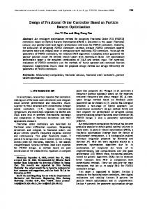
The differential equation of the PIλDδ controller in time domain is described by: (2.55) By taking the Laplace transform for the above equation, (2.56) The transfer function of the FOPID controller in s-domain is; (2.57) If taking λ = δ = 1, a conventional integer-order PID controller is obtained, if λ=0, δ=1, a conventional integer-order PD controller is obtained, and if λ=1, δ=0, a conventional integer-order PI controller is obtained. With the more freedom in the tuning the orders of FOPID controller, Figure (2.3) illustrates the plane of the integral and derivative actions of the PID controller. Obviously, the classical PID controller can be only represented by four points in the plane, while the FOPID controller is represented by the whole limited plane [26].

Chapter Two:


λ (2,2)

(0,2) (0,1) PI

(1,1) PID (1,0)

P

PD

(2,0) δ

Figure (2.3) The order of derivative and integral of PID and FOPID: From point to plan[31]

For the FOPID controller, besides selecting Kp, Ki, and Kd, it needs to select λ and δ which are not necessary integer numbers [32]. The searching operation of the five parameters which can be done through an optimization method makes the design scenario of the FOPID controller is more challenging than the conventional PID controllers. Several methods have been proposed for this design by using optimization methods [32].

v The Root Locus of Fractional Transfer Function The most popular and powerful tools for both analysis and design of single-input single-output (SISO) linear time-invariant (LTI) systems is the root-locus method. There are two main application areas for this method as follows. The first one is the stability: to obtain sufficient conditions on a real parameter K under which the closed-loop system in Figure (2.4) remains stable. The second is the compensator design: the root-locus method offers an efficient tool for the design of lead-lag compensators [33, 34].

Chapter Two:


K

Figure (2.4) Standard closed-loop system

To understand the root locus of fractional order system, one must know some definitions such as: Riemann surface: the two or more s planes that do not cross a cat, but pass continuously from one plane to the other if these s planes are joined in this way is called Riemann surface. In other words, a multilayered surface in the theory of complex functions on which a multi valued complex function can be treated as a single valued function of a complex variable [35]. Riemann sheet: Each s plane of a Riemann surface is called Riemann sheet or any complex functions that the values put in the run -π< θ 1)

(2.65)

Note that the domain of definition of P(s) is a Riemann surface with δ Riemann sheets. From 1+k P (s) =0, when k is a positive real constant, the poles and zeros can be calculated, some of these poles and zeros are put in the first Riemann sheet (FRS) and only these poles and zeros affected on the stability of the system [33,34]. If the fractional-order polynomial D(s) is not minimal, the number of the poles is increased, but the location of poles and the order (degree {D (s)} are unchanged. For example, if the fractional-order polynomial D (s) =s1/2-1 (is minimal) and G (s) = s2/4-1 (is not minimal), then the equation D (s) =0 has only one root at s = ei0 (on the first Riemann sheet), while G (s) = 0 has a same root at s =ei0 (on the first Riemann sheet) and other root at s =e i4π (on the third Riemann sheet). The characteristic equation of the closed-loop system of Figure (2.4) is

(2.66) It is desired to address the generalized root-locus problem that is to plot the root loci of the first Riemann sheet poles and zeros (2.66) when k varies. Note that the time domain behavior and stability properties of the closed-loop system are determined only by the roots that lie on the first Riemann sheet.

Chapter Two:


The system is stable, if and only if, all roots are in the closed left half plane (CLHP) of the first Riemann sheet poles and zeros [33]. To solve this problem, replacing every s1/δ with w gives,

1

+ 2

+

=0

(2.67)

The relationship between w-plane and sheets of the s Riemann surface can be explained by the Figure (2.6) that is the sector to FRS and the stable pole region in

corresponds .

Im s s1

Im w Sheet 1

Re s

Stable region Unstable region

The s-plane of first pole in the first sheet Im s

Sheet 2

s2

Sheet 2

Re s

Sheet 1

Re w

Stable region Stable region

The s-plane of second pole in the second sheet

The w-plane of system has two sheets (2.6.a) The s-plane of the system

(2.6.b) The w-plane of the system

Figure (2.6) The correspondence between w-plane and s Riemann sheets where the number of Riemann sheets = δ = 2.

Chapter Two:


The algorithm of the root locus is as follows; 1- Find the characteristic equation of the closed loop as equation (2.60). 2- Find the least common multiple for the fractional order of the nominator and denominator of the plant. 3- Divide the fractional order of the nominator and denominator of the plant by the least common multiple (let the least common multiple=δ). 4- Exchange from s-plane tow-plane and that is means exchange the s1/δ to w, in another word w= s1/δ. 5- Find the roots of the characteristic equation of w-plane when k changes from zero to infinity. 6- Apply s= wδ exchange from w-plane to s-plane for the poles in the first Riemann sheet FRS only

(Because only these poles

effected on the stability) 7- Plot the poles of the first Riemann sheet FRS only in the Real and Imaginary axis . vi Bode Plot for Fractional Orders Transfer Function The method to calculate the frequency response of fractional order transfer function is same as the frequency response of integer order transfer function [26]. Let,

(2.68)

Then,

(2.69) (2.70) (2.71)

The gain in decibel shall be;

Chapter Two:


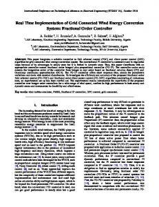
(2.72) The bode plot of order fractional transfer function

is shown in the

Figure (2.7), where α > 0 and α < 0.

20α dB/dec

0

1

20α dB/dec

0

ω red/s

απ

ω red/s

0

/2 0

ω red/s

1

απ

ω red/s a. α > 0

/2 b. α < 0

Figure (2.7) The bode diagrams of fractional order transfer function

vii Nyquist for Fractional Orders Transfer Function The stability rules and the plot of Nyquist for fractional order transfer function is same as the stability rules and the plot of Nyquist for integer order transfer function. 2. 3 Particle Swarm Optimization (PSO) The PSO algorithm was originally proposed by Kennedy and Eberhart in 1995 [9]. The PSO is the abbreviation of Particle swarm optimization. It depends on the behavior of a colony or swarm of insects, such as bees, termites, ants, and wasps or a school of fishes or a flock of birds. The PSO algorithm mimics the behavior of these social organisms. The word particle represents a bee in a colony or a bird in a flock. Each individual or particle in

Chapter Two:


a swarm behaves in a distributed way using its own intelligence and the collective or group intelligence of the swarm. As an example, if one particle found a good path for food, the rest of the swarm would also be able to follow the good path instantly, even if their locations in the swarm were far away from the path. PSO optimization methods based on swarm intelligence are called behaviorally inspired algorithms instead of the genetic algorithms, which are called evolution-based procedures [36]. In the context of multivariable optimization, the swarm is assumed to be of a specified or fixed size with each particle located initially at random locations in the multidimensional design space. Each particle initially assumed to have two characteristics: a position and a velocity. Each particle wanders around in the design space and remembers the best position (in terms of the food source or objective function values) which is discovered by it. The particles communicate information or good positions to each other, and accordingly adjust their individual positions and velocities based on the information received about the best positions [37]. Consider the behavior of birds in a flock. Although each bird has a limited intelligence by itself, it follows the following simple rules: 1. The bird is trying to not be close to other birds. 2. The bird is trying to head towards the average direction of other birds. 3. It tries to fit the "average position" among other birds with no large gaps in the flock. Thus, the behavior of the flock or swarm is based on a combination of three simple factors: 1. Cohesion—sticks together. 2. Separation—doesn’t come too close. 3. Alignment—follows the general heading of the flock. The PSO is developed based on the following model:

Chapter Two:


1. If one bird finds the target or the food (or the maximum of the objective function), it immediately transmits the information to all other birds. 2. All other birds will receive information and will be attracted to the target or the food (or the maximum of the objective function), but not directly. The particle velocity and position of the standard PSO can be updated by the following equations:

(2.73) (2.74) Where

is the velocity of the jth particle at (i) iterations,

position of the jth particle at (i) iterations,

and

is the

are the cognitive

(individual) and social (group) learning rates, respectively,

1 and

2

are uniformly distributed random numbers in the range 0 to 1 and N is the number of particles in swarm [9]. Figure (2.8) shows the trajectory of the particle in the swarm.

previous velocity Current position

new position

Pbest new velocity

Optimal solution

gbest Figure (2.8) The trajectory of the particle after velocity updating

There are different types of improvement to the PSO algorithm and in this thesis using weight method. It turns out that the particle velocities usually build up very fast and skip the maximum of the objective function. Hence, an inertia term W is added to reduce the speed. Usually, the assumed value of W

Chapter Two:


varies linearly from 0.9 to 0.4 as the iterative process progresses. The speed of the particles in swarm with the term of inertia is [10,19],

(2.75) The inertia weight W was introduced by Shi and Eberhart in 1999 [37]. The inertia weight W was added to the velocity equation to dampen the velocities over time (or iterations). This damping is enabling the swarm to converge more accurately and efficiently compared to the original PSO algorithm. This addition improves the fine tuning ability of the PSO to find precise solutions. A larger value of W enhances the global exploration of the PSO, while a smaller value of W enhances the local search. Thus, a large value of W makes the algorithm is constantly exploring new areas without much local search, and hence fails to find the true optimum. To achieve a balance between global and local exploration and to speed up convergence to the true optimum, the value of an inertia weight has to decrease linearly with the iterations’ number, as shown in equation (2.70):[10] (2.76) Where,

is the maximum value of the inertia weight,

minimum value of the inertia weight,

is the maximum number of

iterations used in PSO and i is the current iteration. The value of and

is the

= 0.4 are commonly used.

The flow chart of PSO is illustrated in Figure (2.9).

= 0.9

Chapter Two:

PID Controller and Searching Method: 32 Start

Initialize the positions for each particle and the velocities =0 Evaluate cost value of each particle For each particle set local best cost =current objective function Local best position = current position

Set global best objective function = min (for all local best objective functions)

Update the positions and velocities for each particles using position and velocity update equation

Evaluate objective function t value of each particle

No

For each particle If current cost