Hindawi Publishing Corporation Mathematical Problems in Engineering Volume 2013, Article ID 419043, 7 pages http://dx.doi.org/10.1155/2013/419043
Research Article Design Optimization of a Speed Reducer Using Deterministic Techniques Ming-Hua Lin,1 Jung-Fa Tsai,2 Nian-Ze Hu,3 and Shu-Chuan Chang2,4 1
Department of Information Technology and Management, Shih Chien University, No. 70, Dazhi Street, Taipei 10462, Taiwan Department of Business Management, National Taipei University of Technology, No. 1, Section 3, Chung-Hsiao E. Road, Taipei 10608, Taiwan 3 Department of Information Management, No. 64, Wunhua Road, Huwei Township, Yunlin County 632, Taiwan 4 Department of Information Management, St. John’s University, No. 499, Section 4, Tam King Road, Tamsui District, New Taipei City 25135, Taiwan 2
Correspondence should be addressed to Jung-Fa Tsai;
[email protected] Received 26 June 2013; Accepted 10 September 2013 Academic Editor: Yi-Chung Hu Copyright © 2013 Ming-Hua Lin et al. This is an open access article distributed under the Creative Commons Attribution License, which permits unrestricted use, distribution, and reproduction in any medium, provided the original work is properly cited. The optimal design problem of minimizing the total weight of a speed reducer under constraints is a generalized geometric programming problem. Since the metaheuristic approaches cannot guarantee to find the global optimum of a generalized geometric programming problem, this paper applies an efficient deterministic approach to globally solve speed reducer design problems. The original problem is converted by variable transformations and piecewise linearization techniques. The reformulated problem is a convex mixed-integer nonlinear programming problem solvable to reach an approximate global solution within an acceptable error. Experiment results from solving a practical speed reducer design problem indicate that this study obtains a better solution comparing with the other existing methods.
1. Introduction Many engineering design problems are formulated as mathematical programming models. In last few decades, these nonlinear engineering problems have been investigated in much research that solved the formulated problems by different methods. The methods can be generally categorized into metaheuristic and deterministic approaches. To compare the performance of different optimization algorithms, several structural engineering applications are often solved to validate or test the suitability of the optimization algorithms. The speed reducer problem is one of the benchmark problems in structural optimization. The problem represents the design of a simple gear box used in a light airplane between the engine and propeller to allow each to rotate at its most efficient speed. A large number of algorithms have been developed to solve different engineering optimization problems. In order
to overcome the computational drawbacks of existing numerical methods, many metaheuristic algorithms that combine rules and randomness to imitate natural phenomena [1] have been developed. The most general metaheuristic methods include evolutionary computation (EC), tabu search (TS), simulated annealing (SA), ant colony optimization (ACO), and particle swarm (PS) [2]. The surveys of applications and algorithmic advances for metaheuristic algorithms are provided by Glover and Kochenberger [3], Lee and Geem [1], and Bianchi et al. [4]. Li and Papalambros [5] used the global optimization knowledge that is incorporated in several types of rules concerning constraint activity, redundancy, and dominance to solve the speed reducer problem. Ku et al. [6] solved the speed reducer problem using the Taguchi method that emphasizes the design of a robust product insensitive to disturbances. Akhtar et al. [7] developed an optimization algorithm based on a sociobehavioural concept of society and
2
Mathematical Problems in Engineering
civilization to solve the same problem. The essence of their methodology is derived from the concept that the behaviour of an individual changes and improves due to social interaction with the society leaders. Rao and Xiong [8] proposed a hybrid genetic algorithm that combines the advantages of random search and deterministic search methods to improve the convergence speed and computational efficiency for solving mixed-discrete nonlinear design optimization problems. They also solved the speed reducer problem to demonstrate the effectiveness and robustness of their approach. Cagnina et al. [9] developed a particle swarm optimization algorithm to solve constrained engineering optimization problems and used four standard engineering design problems including a speed reducer problem to validate their algorithm. Jaberipour and Khorram [2] proposed two new harmony search (HS) metaheuristic algorithms for engineering optimization problems with continuous design variables and applied their method to solve the speed reducer problem. Although the metaheuristic algorithms have the advantages of broad applicability, easy implementation, and robustness, these methods cannot guarantee global optimality of the solution. Several deterministic approaches based on mathematical programming techniques have been developed to solve engineering design problems. Tosserams et al. [10] proposed a decomposed problem formulation based on the augmented Lagrangian penalty function and the block coordinate descent algorithm for quasiseparable multidisciplinary design optimization problems. They solved the speed reducer design problem by the proposed decomposition algorithms. Lu and Kim [11] proposed a decomposition algorithm for the multidisciplinary design optimization problems with complementarity constraints based on the regularization technique and inexact penalty decomposition. They also solved the design problem of a speed reducer. One major deterministic approach to globally solve generalized geometric programming problems is to reformulate the original problems into convex mixed-integer nonlinear programming (MINLP) problems. Some transformation techniques have been developed to convexify the nonconvex functions. P¨orn et al. [12] introduced different convexification strategies to deal with posynomial and negative binomial terms. Floudas and Pardalos [13] and Maranas and Floudas [14] proposed exponential transformations to treat nonconvex terms. Lundell et al. [15] proposed some transformation techniques to solve optimization problems including signomial functions to global optimality. Li and Lu [16] applied convexification strategies and piecewise linearization techniques to solve generalized geometric programming problems with free discrete/continuous variables. Tsai and Lin [17] proposed an efficient method to solve a posynomial geometric programming problem with separable functions by applying an appropriate variable transformation and an efficient piecewise linearization formulation. Lin et al. [18] used convexification strategies and piecewise linearization techniques to solve engineering optimization problems including the speed reducer design problem. Lu [19] proposed a convexification transformation method (beta method) based on the concept of 1-convex functions to improve the efficiency of solving generalized geometric programming problems. Huang [20] proposed
x7
x4 x2
x3
x5 x1
x6
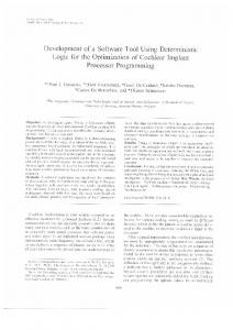
Figure 1: Speed reducer design [24].
a deterministic optimization approach to solve geometric programming problems including the speed reducer design problem. His method converts all signomial terms into convex and concave terms, and then the concave terms are further treated with a piecewise linearization method. Lin and Tsai [21] also used convexification strategies and piecewise linearization techniques to solve the speed reducer design problem. This study applies an efficient optimization approach to globally solve speed reducer design problems based on deterministic techniques. In addition to convexification strategies and piecewise linearization techniques, this study applies optimization-based range reduction techniques [22, 23] to improve computational efficiency in globally solving the speed reducer design problem. Compared with existing methods, the proposed method is capable of obtaining a better solution. The rest of the paper is organized as follows. Section 2 describes the process of globally solving a speed reducer design problem. A practical speed reducer problem is solved in Section 3 to demonstrate the effectiveness of the proposed method. After that, conclusion remarks are made in Section 4.
2. Global Optimization Approach of a Speed Reducer Design Problem A speed reducer is part of the gear box of mechanical system, and it is used in many other types of applications. The design of the speed reducer is a more challenging benchmark, because it involves seven design variables [25]. As shown in Figure 1, the design of the speed reducer is considered with the face width (𝑥1 ), the module of the teeth (𝑥2 ), the number of teeth on pinion (𝑥3 ), the length of the first shaft between bearings (𝑥4 ), the length of the second shaft between bearings (𝑥5 ), diameter of the first shaft (𝑥6 ), and the diameter of the second shaft (𝑥7 ). Another schematic of the speed reducer is presented in Figure 2 with its design variables being labeled. This problem is taken from Golinski [26]. The objective is to minimize the total weight of the speed reducer while satisfying eleven constraints. The constraints include the limits on the bending stress of the gear teeth, surface stress, transverse deflections of shafts 1 and 2 due to transmitted force, and stresses in shafts 1 and 2. The mathematical
Mathematical Problems in Engineering
3 1.5𝑥6 + 1.9 − 1 ≤ 0, 𝑥4 1.1𝑥7 + 1.9 𝑔11 = − 1 ≤ 0, 𝑥5
𝜙x6
𝑔10 =
x3 : number of teeth x2 : tooth model 𝜙x7 Shaft 2
Bearing 2 x4 x5
2.6 ≤ 𝑥1 ≤ 3.6,
Gear 1
17 ≤ 𝑥3 ≤ 28,
x1
0.7 ≤ 𝑥2 ≤ 0.8, 7.3 ≤ 𝑥4 ≤ 8.3,
7.3 ≤ 𝑥5 ≤ 8.3,
2.9 ≤ 𝑥6 ≤ 3.9,
5 ≤ 𝑥7 ≤ 5.5. Bearing 1
Gear 2
Figure 2: A schematic of the speed reducer [11].
programming model of a speed reducer problem considered in this study is expressed as follows. Minimize
(1)
Shaft 1
The original speed reducer problem described previously can be simplified as the following generalized geometric programming problem. Minimize
𝑓 (𝑥1 , . . . , 𝑥7 )
+ (0.7854 × 14.9334) 𝑥1 𝑥22 𝑥3
= 0.7854𝑥1 𝑥22 × (3.3333𝑥32
− (0.7854 × 43.0934) 𝑥1 𝑥22 + 14.9334𝑥3 − 43.0934)
− 1.508𝑥1 𝑥62 − 1.508𝑥1 𝑥72 + 7.4777𝑥63 + 7.4777𝑥73 + 0.7854𝑥4 𝑥62 + 0.7854𝑥5 𝑥72 ,
− 1.508𝑥1 (𝑥62 + 𝑥72 ) + 7.4777 (𝑥63 + 𝑥73 ) + 0.7854 (𝑥4 𝑥62 subject to
𝑓 (𝑥1 , . . . , 𝑥7 ) = (0.7854 × 3.3333) 𝑥1 𝑥22 𝑥32
+
𝑥5 𝑥72 ) ,
subject to
𝑔1 = 27𝑥1−1 𝑥2−2 𝑥3−1 − 1 ≤ 0, 𝑔2 = 397.5𝑥1−1 𝑥2−2 𝑥3−2 − 1 ≤ 0,
𝑔1 =
27 − 1 ≤ 0, 𝑥1 𝑥22 𝑥3
𝑔3 = 1.93𝑥43 𝑥2−1 𝑥3−1 𝑥6−4 − 1 ≤ 0,
𝑔2 =
397.5 − 1 ≤ 0, 𝑥1 𝑥22 𝑥32
𝑔5 = 7452 𝑥42 𝑥2−2 𝑥3−2 − 1102 𝑥66 + 16.9 × 10⁶
1.93𝑥43 − 1 ≤ 0, 𝑔3 = 𝑥2 𝑥3 𝑥64 𝑔4 =
1.93𝑥53 𝑥2 𝑥3 𝑥74
𝑔5 =
745𝑥4 2 1 √ ( ) + 16.9 × 10⁶ − 1 𝑥2 𝑥3 110𝑥63
− 1 ≤ 0,
≤ 0, 𝑔6 =
745𝑥5 2 1 √ ( ) + 157.5 × 10⁶ − 1 𝑥2 𝑥3 85𝑥73
≤ 0, 𝑔7 =
𝑥2 𝑥3 − 1 ≤ 0, 40
5𝑥 𝑔8 = 2 − 1 ≤ 0, 𝑥1 𝑥 𝑔9 = 1 − 1 ≤ 0, 12𝑥2
𝑔4 = 1.93𝑥53 𝑥2−1 𝑥3−1 𝑥7−4 − 1 ≤ 0, ≤ 0, 𝑔6 = 7452 𝑥52 𝑥2−2 𝑥3−2 − 852 𝑥76 + 157.5 × 10⁶ ≤ 0, 𝑔7 = 𝑥2 𝑥3 − 40 ≤ 0, 𝑔8 = 5𝑥2 − 𝑥1 ≤ 0, 𝑔9 = 𝑥1 − 12𝑥2 ≤ 0, 𝑔10 = 1.5𝑥6 − 𝑥4 + 1.9 ≤ 0, 𝑔11 = 1.1𝑥7 − 𝑥5 + 1.9 ≤ 0, 2.6 ≤ 𝑥1 ≤ 3.6, 17 ≤ 𝑥3 ≤ 28, 7.3 ≤ 𝑥5 ≤ 8.3,
0.7 ≤ 𝑥2 ≤ 0.8, 7.3 ≤ 𝑥4 ≤ 8.3, 2.9 ≤ 𝑥6 ≤ 3.9,
5 ≤ 𝑥7 ≤ 5.5. (2) The simplified problem above is a nonconvex program. Based on the deterministic techniques, this study transforms the problem into a convex MINLP problem by the convexification strategies and piecewise linearization methods. Then
4
Mathematical Problems in Engineering
the reformulated problem can be solved by convex MINLP solvers to obtain a global optimal solution. First, we determine that certain classes of signomial terms in the above simplified problem are convex and do not necessitate any transformations. Consequently, the number of concave functions requiring to be piecewise linearized decreases, and the resulting problem is a computationally efficient model. 𝑥63 and 𝑥73 are convex terms. According to Maranas and Floudas [27], 𝑥1−1 𝑥2−2 𝑥3−1 and 𝑥1−1 𝑥2−2 𝑥3−2 are also convex terms. Then, the nonconvex monomials are transformed. By taking exponential transformation [28, 29] on the variable with a positive exponent, the positive monomial terms 𝑥1 𝑥22 𝑥32 , 𝑥1 𝑥22 𝑥3 , 𝑥4 𝑥62 , 𝑥5 𝑥72 , 𝑥43 𝑥2−1 𝑥3−1 𝑥6−4 , 𝑥53 𝑥2−1 𝑥3−1 𝑥7−4 , 𝑥42 𝑥2−2 𝑥3−2 , 𝑥52 𝑥2−2 𝑥3−2 , and 𝑥2 𝑥3 are transformed into convex terms 𝑒𝑦1 +2𝑦2 +2𝑦3 , 𝑒𝑦1 +2𝑦2 +𝑦3 , 𝑒𝑦4 +2𝑦6 , 𝑒𝑦5 +2𝑦7 , 𝑒3𝑦4 𝑥2−1 𝑥3−1 𝑥6−4 , 𝑒3𝑦5 𝑥2−1 𝑥3−1 𝑥7−4 , 𝑒2𝑦4 𝑥2−2 𝑥3−2 , 𝑒2𝑦5 𝑥2−2 𝑥3−2 , and 𝑒𝑦2 +𝑦3 , respectively, where 𝑦𝑖 = ln 𝑥𝑖 , 𝑖 = 1, 2, . . . , 7. By taking power transformations [28–32] on the variables to make the sum of the exponents not greater than one, the negative monomial terms −𝑥1 𝑥22 , −𝑥1 𝑥62 , −𝑥1 𝑥72 , −𝑥66 , and −𝑥76 are transformed into convex terms −𝑧11/3 𝑧22/3 , −𝑧11/3 𝑧61/3 , −𝑧11/3 𝑧71/3 , −𝑧6 , and −𝑧7 , respectively, where 𝑧𝑖 = 𝑥𝑖3 , 𝑖 = 1, 2, 𝑧𝑖 = 𝑥𝑖6 , 𝑖 = 6, 7. The nonconvex problem can be convexified and underestimated by the convexification strategies mentioned previously if the inverse transformations (𝑦𝑖 = ln 𝑥𝑖 , 𝑖 = 1, 2, . . . , 7, 𝑧𝑖 = 𝑥𝑖3 , 𝑖 = 1, 2, and 𝑧𝑖 = 𝑥𝑖6 , 𝑖 = 6, 7) are approximated by piecewise linear functions. The efficiency of the piecewise linearization technique has a critical impact on the computational efficiency in solving the reformulated problems. Vielma and Nemhauser [33] proposed a linearization approach that has favorable tightness properties. Their experimental results showed that the Vielma and Nemhauser [33] method significantly outperforms other models. Tsai and Lin [17] employed the Vielma and Nemhauser [33] method to solve posynomial geometric programming problems. This study also adopts the Vielma and Nemhauser [33] method to linearly approximate the inverse transformations. Compared with the Lin and Tsai [21] method, this study utilizes range reduction techniques [22, 23] to further improve the computational efficiency. Adding more break points can construct a tighter underestimator of the original problem, and the obtained solution is more closer to the real global solution. If 𝑔𝑖 (𝑥) < 0 is the 𝑖th constraint and 𝑥∗ is the solution derived from the reformulated model, then the number of break points does not need to increase until Max𝑖 (𝑔𝑖 (𝑥∗ )) ≤ 𝜀, where 𝜀 is the feasibility tolerance.
+ (0.7854 × 14.9334) 𝑒𝑦1 +2𝑦2 +𝑦3
3. Computational Experiments By using the deterministic approach introduced above, this study reformulates the original speed reducer problem as a convex MINLP problem as follows. Minimize
𝑓 (𝑥1 , . . . , 𝑥7 ) = (0.7854 × 3.3333) 𝑒𝑦1 +2𝑦2 +2𝑦3
− (0.7854 × 43.0934) 𝑧11/3 𝑧22/3 − 1.508𝑧11/3 𝑧61/3 − 1.508𝑧11/3 𝑧71/3 + 7.4777𝑥63 + 7.4777𝑥73 + 0.7854𝑒𝑦4 +2𝑦6 + 0.7854𝑒𝑦5 +2𝑦7 , subject to
𝑔1 = 27𝑥1−1 𝑥2−2 𝑥3−1 − 1 ≤ 0, 𝑔2 = 397.5𝑥1−1 𝑥2−2 𝑥3−2 − 1 ≤ 0, 𝑔3 = 1.93𝑒3𝑦4 𝑥2−1 𝑥3−1 𝑥6−4 − 1 ≤ 0, 𝑔4 = 1.93𝑒3𝑦5 𝑥2−1 𝑥3−1 𝑥7−4 − 1 ≤ 0, 𝑔5 = 7452 𝑒2𝑦4 𝑥2−2 𝑥3−2 − 1102 𝑧6 + 16.9 × 10⁶ ≤ 0, 𝑔6 = 7452 𝑒2𝑦5 𝑥2−2 𝑥3−2 − 852 𝑧7 + 157.5 × 10⁶ ≤ 0, 𝑔7 = 𝑒𝑦2 +𝑦3 − 40 ≤ 0, 𝑔8 = 5𝑥2 − 𝑥1 ≤ 0, 𝑔9 = 𝑥1 − 12𝑥2 ≤ 0, 𝑔10 = 1.5𝑥6 − 𝑥4 + 1.9 ≤ 0, 𝑔11 = 1.1𝑥7 − 𝑥5 + 1.9 ≤ 0, 𝑦𝑖 = 𝐿 (ln 𝑥𝑖 ) ,
𝑖 = 1, 2, . . . , 7,
𝑧𝑖 = 𝐿 (𝑥𝑖3 ) ,
𝑖 = 1, 2,
𝑧𝑖 = 𝐿 (𝑥𝑖6 ) ,
𝑖 = 6, 7,
2.6 ≤ 𝑥1 ≤ 3.6, 17 ≤ 𝑥3 ≤ 28, 7.3 ≤ 𝑥5 ≤ 8.3,
0.7 ≤ 𝑥2 ≤ 0.8, 7.3 ≤ 𝑥4 ≤ 8.3, 2.9 ≤ 𝑥6 ≤ 3.9,
5 ≤ 𝑥7 ≤ 5.5. (3) In the transformation process, the piecewise linearization technique introduced by Vielma and Nemhauser [33] is utilized to approximate ln 𝑥𝑖 (𝑖 = 1, 2, . . . , 7), 𝑥𝑖3 (𝑖 = 1, 2), and 𝑥𝑖6 (𝑖 = 6, 7). The Vielma and Nemhauser [33] method represents a piecewise linear function with 𝑚 break points by ⌈log2 𝑚⌉ binary variables. By using 3, 4, . . . , 9 binary variables, respectively, we convert this program to a convex MINLP problem with 8, 16, . . . , 512 break points, respectively, used in linearly approximating the inverse transformations. The reformulated problems are solved by LINGO [34]. Table 1 lists the reported solutions from LINGO, objective values on
Mathematical Problems in Engineering
5
Table 1: Experiment results of the speed reducer problem by the proposed method under different numbers of break points. No. of break points
No. of binary variables
Reported solution (𝑥1 , 𝑥2 , 𝑥3 , 𝑥4 , 𝑥5 , 𝑥6 , 𝑥7 )
CPU time (mm:ss)
Objective value
Error in constraint
3 4 5 6 7 8 9
(3.5, 0.7, 17.0, 7.3, 7.714826, 3.347398, 5.286205) (3.5, 0.7, 17.0, 7.3, 7.715248, 3.349748, 5.286589) (3.5, 0.7, 17.0, 7.3, 7.715291, 3.350039, 5.286628) (3.5, 0.7, 17.0, 7.3, 7.715313, 3.350187, 5.286648) (3.5, 0.7, 17.0, 7.3, 7.715318, 3.353125, 5.286653) (3.5, 0.7, 17.0, 7.3, 7.715320, 3.350213, 5.286654) (3.5, 0.7, 17.0, 7.3, 7.715320, 3.350214, 5.286654)
00:07 00:09 00:10 00:42 01:27 05:23 15:09
2993.457535 2994.308994 2994.408856 2994.459757 2994.467375 2994.470348 2994.470603
0.002526473 0.000418000 0.000157319 0.000024774 0.000009551 0.000001492 0.000000596
8 16 32 64 128 256 512
Table 2: Experiment results of the speed reducer problem by the proposed method with range reduction. Iteration
1
2
Variable bound [2.6, 3.6] [0.7, 0.8] [17, 28] [7.3, 8.3] [7.3, 8.3] [2.9, 3.9] [5, 5.5] [3.5, 3.500182] [0.7, 0.700011] [17, 17.000419] [7.3, 7.307746] [7.715291, 7.718508] [3.350039, 3.350290] [5.286628, 5.286654]
Reported solution (𝑥1 , 𝑥2 , 𝑥3 , 𝑥4 , 𝑥5 , 𝑥6 , 𝑥7 )
Accumulated CPU time (mm:ss)
Objective value
Error in constraint
(3.5, 0.7, 17.0, 7.3, 7.715291, 3.350039, 5.286628)
00:10
2994.408856
0.000157319
(3.5, 0.7, 17.0, 7.3, 7.7153190, 3.350282, 5.286654)
07:56
2994.471921
0.000000264
2,994.75 2,994.50
Objective value
2,994.25 2,994.00 2,993.75 2,993.50 2,993.25 2,993.00 2,992.75 8
16
32 64 128 Number of break points
256
512
Figure 3: Objective values of the speed reducer problem under different numbers of break points.
the reported solutions, and errors in constraint Max𝑖 (𝑔𝑖 (𝑥∗ )) under different numbers of break points. Using more break points derives a solution with a lower error in constraint. Figure 3 indicates the objective value obtained from the proposed method under different numbers of break points. We observe that the objective value approximates the real global objective value better as the number of break points increases. Figure 4 indicates the CPU time required to solve
the speed reducer problem under different numbers of break points. The required CPU time to solve the reformulated model tends to grow exponentially as the number of break points becomes large. To enhance computational efficiency, this study applies the range reduction techniques to effectively tighten variable bounds. Table 2 lists variable bound, solution, objective value, accumulated CPU time, and error in constraint in each iteration to solve this problem by the proposed method with range reduction. Thirty-two break points are used in the piecewise linearization process in each iteration. The accumulated CPU time consists of the CPU time to update variable bounds and solve the reformulated models iteratively. The global solution (3.5, 0.7, 17.0, 7.3, 7.7153190, 3.350282, and 5.286654) with objective 2994.471921 and an error in constraint below 10−6 can be obtained within 8 minutes. If no range reduction is adopted and 512 line segments are used in the piecewise linearization process, the global solution with an error in constraint below 10−6 is obtained within 16 minutes as shown in Table 1. Table 3 displays the comparison of results with existing methods. The solutions listed in the table are reported from their original research, and the objective values are computed from the objective function 𝑓(𝑥1 , . . . , 𝑥7 ) = 0.7854𝑥1 𝑥22 (3.3333𝑥32 +14.9334𝑥3 −43.0934)−1.508𝑥1 (𝑥62 +𝑥72 ) + 7.4777(𝑥63 + 𝑥73 ) + 0.7854(𝑥4 𝑥62 + 𝑥5 𝑥72 ) on the reported solutions. Tosserams et al. [10] and Lu and Kim [11] obtained
6
Mathematical Problems in Engineering Table 3: Comparisons of optimal solutions of the speed reducer problem by different methods.
Methods
Method type
Reported solution (𝑥1 , 𝑥2 , 𝑥3 , 𝑥4 , 𝑥5 , 𝑥6 , 𝑥7 )
Objective value
Error in constraint
Ku et al. [6]
Metaheuristic
2876.219475