Design Patterns in Beeping Algorithms

Design Patterns in Beeping Algorithms A. Casteigts, Y. M´etivier, J.M. Robson and A. Zemmari

arXiv:1607.02951v1 [cs.DC] 11 Jul 2016

Universit´e de Bordeaux - Bordeaux INP LaBRI UMR CNRS 5800 351 cours de la Lib´eration, 33405 Talence, France {acasteig, metivier, robson, zemmari}@labri.fr

Abstract. We consider networks of processes which interact with beeps. In the basic model defined by Cornejo and Kuhn [15], which we refer to as the BL variant, processes can choose in each round either to beep or to listen. Those who beep are unable to detect simultaneous beeps. Those who listen can only distinguish between silence and the presence of at least one beep. Stronger variants exist where the nodes can also detect collision while they are beeping (Bcd L) or listening (BLcd ), or both (Bcd Lcd ). Beeping models are weak in essence and even simple tasks are difficult or unfeasible with them. This paper starts with a discussion on generic building blocks (design patterns) which seem to occur frequently in the design of beeping algorithms. They include multi-slot phases: the fact of dividing the main loop into a number of specialised slots; exclusive beeps: having a single node beep at a time in a neighbourhood (within one or two hops); adaptive probability: increasing or decreasing the probability of beeping to produce more exclusive beeps; internal (resp. peripheral) collision detection: for detecting collision while beeping (resp. listening); and emulation of collision detection: for detecting collisions when this feature is not available as a primitive. The paper then provides algorithms for a number of basic problems, including colouring, 2-hop colouring, degree computation, 2-hop MIS, and collision detection (in BL). Using the patterns, we formulate these algorithms in a rather concise and intuitive way. Their analyses are more technical. One of them relies on a Martingale technique with nonindependent variables. Another of our analyses improves that of the MIS algorithm in [24] by getting rid of a gigantic constant (the asymptotic order was already optimal). Finally, we study the relative power of several variants of beeping models. In particular, we explain how every Las Vegas algorithm with collision detection can be converted, through emulation, into a Monte Carlo algorithm without, at the cost of a logarithmic slowdown. We prove this is optimal up to a constant factor by giving a matching lower bound, and provide an example of use for solving the MIS problem in BL.

Keywords. Beeping models, Design patterns, Collision detection, Colouring, 2-hop colouring, Degree computation, Emulation.

1 1.1

Introduction Overview of problems

Beeping models. Distributed computing is concerned with various assumptions, like the structure of the network (trees, rings, planar graphs, etc.) or knowledge available to the nodes (network size, identifiers, port numbering, etc.). Another important aspect is the size of messages, which may range from unbounded, to logarithmic size, to constant size.

As a natural goal is to reduce assumptions as much as possible. Typically, when a problem is solved in some strong model, the community strives to solve it in weaker models. In a recent series of works [15,41,1,23,24,21], new models were explored that are even weaker than constant size messages, namely beeping models. In beeping models, the only communication capabilities offered to the nodes are to beep or to listen. Several variants exist. In [15], a node that beeps is unable to detect whether other nodes have beeped simultaneously. When listening, it can distinguish between silence or the presence of at least one beep, but it cannot distinguish between one and several beeps. In Section 6 of [1], beeping nodes can detect whether other nodes are beeping simultaneously. In [41] and Section 4 of [1], yet another variant is considered where listening nodes can tell the difference between silence, one beep, and several beeps. In this paper, we denote the ability to detect collision while beeping (internal collision) by Bcd and that of detecting collision while listening (peripheral collision) by Lcd . The absence of such ability is denoted by B and L, respectively. The various existing models can be reformulated using the cartesian product of these capabilities. Hence, the basic model introduced by Cornejo and Kuhn in [15] is BL; the model considered by Afek et al. in [1] (Section 6) and Jeavons et al. in [24] is Bcd L; and the model considered in [41] and in Section 4 of [1] is BLcd . To the best of our knowledge, Bcd Lcd was only used in a previous work by the authors [11]. Although some variants are stronger than others, all beeping models remain extremely weak in essence. Yet, they are relevant to account for real-world applications or phenomena. For instance, they reflect the features of a network at the lowest levels (physical and MAC layers), where a node can probe or emit signals, with or without collision detection. At a higher level of abstraction, beeping models also reflect some communication patterns in biology [14,1,39]. Investigated Problems. Usually, the topology of a distributed system is modelled by a graph and paradigms of distributed systems are represented by classical problems in graph theory such as vertex degree, MIS1 , 2-hop MIS (we recall that a 2-hop MIS of a graph G is a MIS of the square of G, i.e., the graph with the set of vertices of G in which there is an edge between any two different vertices u and v if the distance between u and v in G is at most 2), colouring (a colouring of a graph G assigns colours to vertices such that two neighbours have different colours), 2-hop colouring (as for a 2-hop MIS, a 2-hop colouring of a graph G is a colouring of the square of G). Each solution to one of these problems is a building block for many distributed algorithms: symmetry breaking, topology control, routing, resource allocation or network synchronisation. As explained in [40] (p. 79), a MIS or a colouring enables the construction of schedules such that two neighbouring vertices do not act concurrently. Furthermore, a MIS can help for the decomposition of a network into clusters. A 2-hop MIS makes it possible to assign each vertex to exactly one cluster head. Channel assignment for a radio network with collision-freedom corresponds to a 2-hop colouring of the graph corresponding to 1

Let G = (V, E) be a graph. An independent set of G is a subset I of V such that no two members of I are adjacent. An independent set I is maximal, denoted MIS, if any vertex of G is in I or adjacent to a vertex of I.

2

the network since each colour corresponds to a channel [31]. The importance of 2-hop colouring is also attested by Emek et al. [16], they prove that in an anonymous network any randomised algorithm can be seen as the composition of a randomised 2-hop colouring and a deterministic algorithm. Finally, in an anonymous wireless network there are no port numbers, in this context a 2-hop colouring ensures that no node has two neighbours with the same colour, and colours act as port numberings. One of the aim of this work is the study of the resolution of these problems in the framework of beeping models. 1.2

Contributions

The contributions of this paper are manifold. As a warm-up, we start by identifying generic building blocks (we call them design patterns) which seem to occur often in the design of beeping algorithms. Then we present a number of algorithms for various graph problems, together with their complexity analyses. Depending on the problems, our algorithms are either the first to solve the problems, or they improve upon previous solutions. Finally, we study the relative power of several variants of beeping models and describe emulation techniques to rely on collision detection even if it is not available. Design patterns. We identify a number of common building blocks in beeping algorithms, including multi-slot phases: the fact of dividing the main loop into a (typically constant) number of slots having specific roles (e.g., contention among neighbours, collision detection, termination detection); exclusive beeps: the fact of having a single node beep at a time in a neighborhood (within one or two hops, depending on the needs); adaptive probability: increasing or decreasing the probability of beeping in order to maximise the number of exclusive beeps; internal (resp. peripheral) collision detection: the fact of detecting collision while beeping (resp. listening); and emulation of collision detection: the fact of detecting collisions even when it is not available as a primitive. As we show in the paper, these patterns make it possible to formulate the algorithms in a rather concise and elegant way. Algorithms and analyses for basic graph problems. We present, or analyse algorithms for a number of basic graph problems, including colouring, 2-hop colouring, degree computation, MIS and 2-hop MIS. For each of the algorithms, we characterise (an upper bound on) its time complexity. All analyses are put together in a dedicated section to maintain a smooth reading of the other parts. More often than not, the design of algorithms is easier and more natural if collision detection is assumed as a primitive, e.g., in Bcd Lcd or Bcd L. Furthermore, emulation techniques such as those described later in this paper enable safe and automatic translations of algorithms into weaker models like BL. For this reason, our algorithms are expressed using whichever model is the most convenient. We first present and analyse a Las Vegas (i.e. guaranteed result, uncertain time) colouring algorithm in the Bcd L model, with time complexity of O(log n + ∆) slots, where ∆ is the maximum degree in G. We prove this bound both on average and with 3

high probability (w.h.p.), that is, with probability 1 − o(n−1 ). (In this particular case, we also prove an even a stronger bound of 1 − o (n−c ), for any c > 1.) The analysis relies on a martingale technique with non-independent random variables, which makes use of a result by Azuma [4]. In fact, the phenomenon we analyse is quite general in beeping models: we characterise the first moment when every node has produced an exclusive beep at least once within its (1-hop) neighbourhood. The main difficulty in this analysis arises from the adaptive probability pattern mentioned above. Another algorithm for 2-hop colouring is given, this time in the Bcd Lcd model, with slot complexity O(log n + ∆2 ) w.h.p. Both algorithms require no knowledge on G. However, both can result in arbitrarily many colours (in fact, as much as the number of slots). If the nodes know an upper bound K ≥ ∆, we propose a different strategy that uses at most K + 1 colours. However, the slot complexity becomes O(K(log n + log2 K)) w.h.p. for colouring (trade K for K 2 in the 2-hop variant). The corresponding analysis is not tight and the real complexity is thought to be lower. These results are summarised on Table 1. A comparison with other algorithms is given in the last section of the paper.

Model Time (# slots) Message size Knowledge # colours This paper Bcd L O(log n + ∆) ≃ 1 bit None O(log n + ∆) expected and w.h.p.
(Bcd L beeps) This paper Bcd L O K(log n + log2 K) ≃ 1 bit Upper bound K on K w.h.p. (Bcd L beeps) the max degree of G Table 1. Randomised Las Vegas colouring algorithms on graphs with n vertices.

Based on the observation that degree computation is strongly related to 2-hop colouring, we present an adaptation of the algorithm for this problem, with same slot complexity, that is, O(log n + ∆2 ) w.h.p. In fact, the analysis of both problems is almost the same as that of colouring, but considered in the square of the graph (whence the ∆2 term). One difference is that the main loop contains more specialised slots (e.g., one for peripheral collision reporting), but still a constant number of them, which keeps the asymptotics unchanged. We then turn our attention to the 2-hop MIS problem, which shares common traits and patterns with 2-hop colouring and degree computation. Here, however, the running time is significantly faster (and the analysis quite different) due to the fact that an exclusive beep causes the whole neighborhood to terminate at once. In fact, we prove that the slot complexity of this algorithm is O(log n) w.h.p. with a “reasonable” constant factor of 76. Noteworthily, the number of phases (i.e. iterations of the main loop) for the 2-hop MIS is the same as what the analogue for classical MIS algorithm would produce in the square of the graph. As a consequence, our analysis substantially improves that of the MIS algorithm presented in [24], where a gigantic constant factor (i.e. one larger than e25 ) is used. An earlier analysis in [42] yielded a better, yet huge constant of 2 × 1011 (see Table 2). Although constant factors are less meaningful in general, the gap in this case is one between practical and unpractical run4

ning times. Furthermore, the contribution it not as much in the constant itself than in the analysis techniques that achieve it (presented in Section 5). Analysed by

Model Time (# slots/rounds)

Scott et al. [42]

Bcd L c log n, with c ≥ 2 × 1011

Jeavons et al. [24] Bcd L ≤ c log n, with c ≥ e25 This paper

Bcd L ≤ c log n, with c = 76

Table 2. Different analyses of the complexity of Scott et al. MIS algorithm.

Collision detection and emulation techniques. Classical considerations on symmetry breaking in anonymous beeping networks, see for example [1] (Lemma 4.1), imply that there is no Las Vegas internal collision detection algorithm in the beeping models BL and BLcd . Likewise, there is no Las Vegas peripheral collision detection algorithm in the beeping models BL and Bcd L. Since collision detection is required to detect exclusive beeps with certainty, and this pattern is central in most beeping algorithms, this implies that a large range of algorithms cannot exist in a Las Vegas version in these models. We study the cost of detecting collision when it is not available, typically in BL, and present generic techniques to emulate collision detection probabilistically in order to transform Las Vegas algorithms with collision detection into Monte Carlo algorithms (uncertain result, guaranteed time) in BL. These techniques generalise that of Algorithm 3 in [1], where a similar strategy is encapsulated into the algorithm. We show how, given 0 < ǫ < 1, any collision in the neighborhood of a given node can be detected in O(log( 1ǫ )) slots with error at most ǫ, and similarly it can be detected in O(log n) slots w.h.p. Ensuring that this is true for any node requires more time. By union bound, it holds that O(log( nǫ )) slots are sufficient with error ǫ and that O(log n) slots are sufficient w.h.p. We prove that this technique is essentially optimal (asymptotically and up to a constant factor) by giving a matching lower bound. Precisely, we prove that some topologies require Ω(log n) slots to break symmetries w.h.p. We provide two generic procedures that can be used in an algorithm to emulate collision detection when it is not available (e.g. in BL). These procedures are EmulateBcdinBL(), to detect collision while beeping, and EmulateLcdinBL(), to detect collision while listening. We illustrate their use in the case of the computation of a MIS given in Bcd L, thus obtaining a Monte Carlo algorithm in BL.

1.3

Organisation of the paper

In Section 2 we present the model and give further definitions. Section 3 introduces design patterns in a tutorial manner. These patterns are then used in Section 4 to describe the various algorithms. For the sake of readability, the corresponding analyses 5

are put together in Section 5. Finally, Section 6 presents our contribution on collision detection and emulation techniques. An extra bibliography is provided in Section 7 on related questions.

2

Network Model and Definitions

We consider a wireless network and we follow definitions given in [1] and [15]. The network is anonymous: unique identifiers are not available to distinguish the processes. Possible communications are encoded by a graph G = (V, E) where the nodes V represent processes and the edges E represent pairs of processes that can hear each other. We denote by ∆ the maximum degree of G. The neighbourhood of a vertex v, denoted N (v), is the set of vertices adjacent to v (at distance 1 from v). We define N (v) by including v itself in N (v). We also use the set of vertices at distance at most 2 from v called the 2-neighbourhood of v and denoted N2 (v) (or N2 (v) if it includes v). Finally, we write log n for the binary logarithm of n. Time is divided into discrete synchronised time intervals (rounds) also called slots (following the usual terminology in wireless networks). All processes wake up and start computation in the same slot. In each slot, all processors act in parallel and either beep or listen. In addition, processors can perform an unrestricted amount of local computation in-between two slots (in effect, our algorithms require little computation). Remark 1. In general, nodes are active or passive. When they are active they beep or listen; in the description of algorithms we say explicitly when a node beeps meaning that a non beeping active node listens. The time complexity, also called slot complexity, is the maximum number of slots needed until every node has terminated. Our algorithms are typically structured into phases, each of which corresponds to a small (constant or logarithmic) number of slots. In the algorithm, we specify which one is the current slot by means of a switch instruction with as many case statements as there are slots in the phase. Phases repeat until some condition holds for termination. Remark 2. An algorithm given in a beeping model induces an algorithm in the (synchronous) message passing model. Thus, given a problem, any lower bound on the round complexity in the message passing model also holds for slot complexity in the beeping model. Distributed Randomised Algorithm. A randomised (or probabilistic) algorithm is an algorithm which makes choices based on given probability distributions. A distributed randomised algorithm is a collection of local randomised algorithms (in our case, all identical). A Las Vegas algorithm is a randomised algorithm whose running time is not deterministic, but still finite with probability 1, and that always produces a correct result. A Monte Carlo algorithm is a randomised algorithm whose running time is deterministic, but whose result may be incorrect with a certain probability. Put differently, Las 6

Vegas algorithms have uncertain execution time but certain result, and Monte Carlo algorithms have certain execution time but uncertain result. Classical considerations on symmetry breaking in anonymous beeping networks (see for instance Lemma 4.1 in [1]), imply that: Remark 3. There is no Las Vegas (and a fortiori no deterministic) algorithm in BL which allows a node to distinguish between an execution where it is isolated and one where it has exactly one neighbour. From this remark we deduce that there is no Las Vegas counting algorithm in BL, which advocates the use of stronger models. In what follows, we consider whichever model is the most convenient and provide Las Vegas algorithms in these models. We then present canonical emulation techniques to turn any such algorithm into a Monte Carlo one in BL.

3

Design patterns for beeping algorithms

As a warm-up, this section presents a number of design patterns which seem to occur frequently in the design of beeping algorithms. The concept of pattern refers here to reusable solutions to common problems. These patterns are then used to describe algorithms in the other sections. Exclusive beeps. Beeping algorithms operate in synchronous periods called slots, which are equivalent to the concept of rounds in message passing models. Most problems in distributed computing require some node v to take exclusive decisions at times (i.e., with respect to vertices of N (v) or N2 (v)), which requires some type of symmetry breaking. In beeping networks, this goal is all the more difficult to achieve that the nodes cannot use identifiers nor even port numbers in their basic exchanges. If we assume that a node that is beeping can detect whether another node beeps simultaneously (Bcd ), then this feature can be used to take exclusive decision if indeed it beeps alone. We call this an exclusive beep. Algorithm 1 illustrates an empty shell of algorithm that relies on repeated attempts to produce exclusive beeps. Most, if not all algorithms rely implicitly on this pattern as a basis.

Algorithm 1: Exclusive beeps (using Bcd ). repeat beep with some probability; if I beeped alone then do something exclusive; ... until f inished;

7

2-hop exclusive beeps. For some problems like 2-hop colouring, 2-hop MIS, or computation of the degree (all discussed in this paper), the level of mutual exclusion offered by exclusive beeps is not sufficient and the algorithm requires that a node be the only one to beep at distance 2. Assuming collision can also be detected upon listening (Lcd ), one can design a 2-slots pattern whereby non-beeping neighbours report if they have heard more than one beep. Hence, if a node produced an exclusive beep in the first slot, and none of its neighbours reported a collision in the second, then it knows that it has produced a 2-hop exclusive beep (see Algorithm 2).

Algorithm 2: Two-hops exclusive beeps (using Bcd Lcd ). repeat switch slot do slot 1 // contending beep with some probability; slot 2 // detection of peripheral collision if several neighbours beeped in slot 1 then beep after slot 2 if I beeped alone in slot 1 and no neighbour beeped in slot 2 then do something 2-hop exclusive ... until f inished;

Multi-slot phases. The example in Algorithm 2 illustrates another common aspect of beeping algorithms, namely multi-slot phases. The expressivity of a single beep is rather poor, but several combined slots can achieve elaborate behavior. In Algorithm 2, one slot is devoted to contending and another to peripheral collision detection. The whole compound is then called a phase. Another common task is termination detection. In a termination slot, all nodes which have not yet performed some action beep. If the slot remain silent, then a form of local termination is detected: nodes are in a terminal state. Adaptive probability. As far as feasibility and expressivity are concerned, the next design pattern is not crucial. However, it plays a central role in terms of performance. Adaptive probability consists in adapting the probability to beep in the next phase depending on the outcome of previous phases. Typically, if a collision occurs, the probability is reduced, and if no one beeps, it is increased. Since the nodes do not know how many neighbours are contending with them, this technique proves useful in optimizing the odds of producing exclusive beeps. The values given to the probabilities in Algorithm 3 are left unspecified. There are several options. In this paper, we use a doubling/halving pattern, that is, p is increased to 2p (up to 1/2), and it is decreased to p/2 (without 8

Algorithm 3: Adaptive beeping probability (using Bcd Lcd ). F loat p ← 1/2 // say repeat beep with probability p; if I beeped alone then do something exclusive; else if no one beeped then increase p; else decrease p; until f inished;

limit). A similar doubling/halving pattern was used in [42]. One could also increment or decrement the denominator of p as done in [11]. The consequences of choosing one over the other are not discussed here. Collision detection. Most algorithms in this paper use collision detection as a built-in primitive, referred to as Bcd for detection on beeping and Lcd for detection on listening. However, this feature is not always available as a primitive. An important question is the transformation of a (high-level) algorithm using Bcd or Lcd (or both) into one that works in the weakest BL model. This question is the topic of Section 6, in which we study generic mechanisms to achieve this goal. Essentially, each slot that requires collision detection can be replaced with a logarithmic number of slots (in the size of various quantities depending on the desired guarantees) where the ties are broken w.h.p. We provide dedicated procedures that generalise the technique used internally to one of the algorithms in [1]. Besides complexity, the price to pay is that the algorithm becomes Monte Carlo instead of Las Vegas, that is, the result is correct only probabilistically (though possibly w.h.p.). We present a matching lower bound showing that these procedures are essentially optimal.

4

Algorithms for basic graph problems

We now present algorithms for a number of problems, including colouring (with or without knowledge on the degree), 2-hop colouring, computation of the degree and 2hop MIS. These algorithms are based on various combinations of the patterns presented in Section 3. All algorithms are Las Vegas, and they rely on medium to strong primitives (Bcd L to Bcd Lcd models) depending on the needs. The adaptation of these algorithms in the weakest model (BL) is discussed in Section 6. We recall also Jeavons et al.’s Las Vegas algorithm for the MIS [24] problem, to which we propose a new analysis in Section 5 that also applies to our 2-hop MIS algorithm. Finally, observe that whenever describing adaptive probability in the algorithms, we keep using the words increase and decrease for generality. The analyses of Section 5 9

instanciate that to a doubling/halving pattern, that is, the probability p of beeping is increased to 2p (up to 1/2), and it is decreased to p/2 (without limit). 4.1

Colouring

The colouring problem consists of assigning a colour to every node in the network, such that no two neighbours have the same colour. We first consider the case that no extra information is available to the nodes. Then we consider that (an upper bound on) the maximum degree is known. Colouring without knowledge. Informally, the algorithm proceeds as follows (see Algorithm 4 for details). Initially, every node is uncoloured (nil). In every phase, each node increments a counter. Uncoloured nodes contend with each other to produce an exclusive beep, and when one succeeds, it takes the current value of the counter as its colour and retires. An adaptive probability is used to regulate the probability of beeping among uncoloured nodes. Local termination (a node and its neighbours are coloured) detection is not explicitly handled here, though we could add a termination slot where uncoloured nodes are the only ones to beep.

Algorithm 4: A Las Vegas colouring algorithm in Bcd L (without knowledge). F loat p ← 1/2; Integer colour ← nil; Integer counter ← 0; repeat beep with probability p; if I beeped alone then colour ← counter else if no one beeped then increase p; else decrease p; counter ← counter + 1; until colour 6= nil;

The running time of this algorithm is analysed in detail in Section 5 (see Theorem 1). We show that the number of phases is O(log n + ∆) w.h.p and on average (none of both imply the other trivially). Note that this is also the number of slots, since each phase consists of a constant number of slots. As for the number of colours, it is incremented with time, thus it is at most the same (at most, because some phases may not produce exclusive beeps). 10

Colouring with a bound K on the maximum degree ∆. If a bound K ≥ ∆ is known, then one can obtain a better colouring using at most K + 1 colours. The algorithm follows the same lines as Algorithm 4, i.e. a colour counter is incremented in each phase, and its current value is chosen by those nodes who produced an exclusive beep. The main difference (see Algorithm 5 for details) is that only those colours within {0, . . . , K} are considered and thus the counter is incremented modulo K + 1. Conflicts of colours are avoided by keeping a phase idle if the corresponding value was already taken in the past (locally). To do so, when a node takes a colour, it re-beeps in a new slot called confirmation slot to inform its neighbours that they must remove the current colour from their list of authorized colours. Accordingly, the uncoloured will contend in a phase only if the current colour is still available (otherwise, they wait). An adaptive probability is used similarly to Algorithm 4, except that idle phases are not considered as silent (the probability is not updated in these phases).

Algorithm 5: A Las Vegas colouring algorithm in Bcd L (knowing K ≥ ∆). Colours = {0, · · · , K}; F loat p ← 1/2; Integer colour ← nil; Integer counter ← 0; repeat if counter ∈ Colours then switch slot do slot 1 // contending beep with probability p slot 2 // confirmation if I beeped alone in slot 1 then colour ← counter; beep; else if no one beeped then increase p; else decrease p; if someone beeped in slot 2 then Colours ← Colours \ {counter} counter ← (counter + 1) mod (K + 1); until colour 6= nil;

Regarding performance, the only difference between this algorithm and Algorithm 4 is that a growing number of phases are idle in each neighbourhood. The analysis thus 11

comes to characterise the slowdown factor induced by these phases compared to the orig-
inal algorithm. We show in Section 5 that the number of phases is O K(log n + log2 K) w.h.p. 4.2

2-hop colouring

A 2-hop colouring of a graph G is a colouring such that any two nodes at distance ≤ 2 have different colours. In other words, it is a colouring of the square of G, the graph where an edge exists between nodes which are neighbours in G or share a common neighbour in G. 2-hop colouring without knowledge. A similar strategy is used as in Algorithm 4 (colouring), except that exclusive beeps are replaced with 2-hop exclusive beeps. Whenever a node produces such a beep, it takes the current value of the counter as colour. Since no other node has beeped within distance 2, the colouring is legal. Contrary to the 1-hop colouring, the collaboration of a node remains crucial even after it becomes coloured. Indeed, this node must keep on reporting peripheral collisions to its neighbours. As a result, instead of retiring from computation, coloured nodes keep on listening until all of their neighbours are coloured, which is detected using an extra termination slot. Details are given in Algorithm 6. Four slots are used in total, the first two being devoted to the management of 2-hop exclusive beeps (see Section 3 for details). The third slot manages a (2-hop) adaptive probability based on beeps heard at distance one (slot 1) or at distance two (slot 3 itself). Finally, slot 4 is the termination slot. Once we realize that the execution produced here is the same as what Algorithm 4 would produce in the square of G, analysis of this algorithm is straightforward. The only difference is that the maximal number of contenders of a node becomes ∆2 instead of ∆. Thus Algorithm 6 takes O(log n + ∆2 ) phases (and slots) w.h.p., and the number of colours cannot exceed that same value. With a bound K on the maximum degree ∆. The same idea can be applied as in the 1-hop case, that is, considering only colours between 0 and K 2 + 1 (instead of K + 1) and incrementing the counter accordingly (modulo K 2 + 1). As a result, at most K 2 + 1 colours are used and the time complexity is O(K 2 (log n + 4 log2 K)) w.h.p. 4.3

Degree computation

Let us recall that 2-hop exclusive beeps allow a node v to perform an exclusive action within a radius of distance 2. This feature was used in Section 4.2 to assign unique colours. At it turns out, the pattern is very versatile and it can be used to count the degree of a node as well. The strategy consists in replacing the colour-related action in slot 2 (second if-then block) by an action aiming at having v counted in the degree of its neighbours (then v stops contending and keeps on reporting collisions, as before). Precisely, a new confirmation slot is inserted wherein v re-beeps if indeed it produced a 2hop exclusive beep. Upon hearing the confirmation beep, all of v’s neighbours increment a local counter that eventually amounts to their degree. Termination proceeds in the same 12

way as for the 2-hop-colouring algorithm (i.e. uncounted nodes beep in a termination slot). Up to a constant factor which accounts for the additional confirmation slot in each phase, the running time of this algorithm is again O(log n + ∆2 ) w.h.p. 4.4

Jeavons et al.’s Las Vegas Algorithm for the MIS in Bcd L

We recall here Jeavons et al.’s Las Vegas Algorithm for the MIS [24]. This algorithm uses an adaptive probability to maximize the frequency of exclusive beeps (with a doubling/halving pattern for p, starting at 1/2). If a node v produces an exclusive beep, it enters the MIS (by the end of the first slot), then it uses a confirmation slot to inform its neighbors, all of which terminate together with v. Since the whole neighborhood shuts down at once, the algorithm progresses faster than, for instance, the basic colouring algorithm discussed above. This algorithm was already proven by Jeavons et al. to terminate within O(log n) with a huge constant factor (larger than e25 ). In Section 5, we propose a new analysis of this algorithm that takes the constant down to 76. 4.5

Computing a 2-hop MIS

As a last example, we solve the 2-hop MIS problem. In this problem, we must select a set of nodes (the MIS) such that no pair of selected nodes are within distance 2 and no node can be added further to the set. This algorithm is a combination of those of other 2-hop algorithms seen above, and Jeavons et al’s MIS algorithm. That is, the same structure of algorithm is used as for 2-hop colouring or degree computation, except that whenever a node produces a 2-hop exclusive beep, it enters the MIS and informs its neighbours (using the confirmation slot) that they will not be in the MIS. This algorithm takes the same number of phases than for the MIS before terminating, that is, O(log n) w.h.p. (see Section 5 for details).

13

Algorithm 6: A Las Vegas 2-hop-colouring algorithm in Bcd Lcd (without knowledge). F loat p ← 1/2; Integer colour ← nil; Integer counter ← 0; repeat switch slot do slot 1 // contending slot if colour = nil then beep with probability p; slot 2 // peripheral collision detection (and consequences) if several neighbours beeped in slot 1 then beep if I beeped alone in slot 1 and heard no beep in slot 2 then colour ← counter slot 3 // adaptive probability if someone beeped in slot 1 then beep if colour = nil then if no beep heard in slot 1 nor 3 then increase p else decrease p slot 4 // termination slot if colour = nil then beep counter ← counter + 1 until no beep heard in slot 4;

14

5

Complexity analysis

This section is devoted to the analysis of algorithms presented in the previous section. 5.1

Colouring algorithm without knowledge

Informally the execution progresses as follows. There is a first period of adjustment in which the probabilities will converge towards “good values”. Then the probability that an exclusive beep is produced in a given phase in a given neighbourhood remains bounded in some ways. Loosely speaking, the final bound is essentially obtained by a repetition of the corresponding periods ∆ times. More precisely, we prove the following theorem: Theorem 1. There are constants α, β and γ such that for any graph G = (V, E) of n vertices and maximum degree ∆, the number of phases of Algorithm 4 to colour all the nodes in G is:
1. less than α(∆ + log n) with probability 1 − o n−1 , 2. less than β(∆ + log n) on average, 3. less than γ(∆ + log n) with probability 1 − o (n−c ), for any c > 1. (This result is stronger than 1, but the proof is more difficult, which is why we keep both.) Local Average Time Complexity. First, we give an overview. We define pv as the probability that vertex v claims the colour in a given round and qv as the sum of p over all neighbours of v which we will call ui (1 ≤ i ≤ d) where d is v’s degree in the residual graph (taken as 0 if v has been eliminated from the graph). We define a measure M of the distance from a given situation to the goal where p = 1/2, qv ≤ 1/2, d = 0 as follows: M = − log(p) + f (q) + 10d where f is the function defined as follows: – f (x) = 4x if x ≤ 1, – for x > 1, f is the piecewise linear approximation to 2 log2 4x wheref is interpolated linearly between f (2i ) = 2i + 4 and f (2i+1 ) = 2i + 6. We note the following properties of f which will be used in what follows: – – – –

f (x) is continuous for x > 0, except at powers of 2, f is differentiable with derivative ≤ 4, f (x) − f (x/2) = 2 for x ≥ 1, f (x) − f (x/2) = 2x for x ≤ 1.

We show that in any round, the mean decrease in M is at least 1. Then after a number of rounds equal to the initial M (≤ 1 + 2 log(2d) + 10d), M is reduced on average to 0 unless the algorithm has already terminated at v and after O(log n) further rounds, the algorithm has terminated at v with probability o(n−2 ) and so it has terminated everywhere with probability o(n−1 ). 15

Intuitively, we expect both p and q to decrease initially until q < 1/2, after which p will re-ascend until it is at least close to 1/2 and then d will start to descend. We actually analyse the variation in a random variable M ′ which dominates the r.v. M . The r.v. M ′ is initially equal to M but its changes may be slightly different from those of M in the following ways: – if the degree of v decreases by more than 1, the change in M ′ only includes −10 in total for the change in d rather than −10 for each neighbour removed; – if v takes a colour, M ′ is decreased by just 10 whatever the values of p at v and its neighbours; – in a round where v is already coloured, M ′ is decreased by 1. This ensures that: – if the algorithm has not terminated at v, M ′ ≥ M , meaning that M ′ dominates M ; – if M ′ ≤ 0, the algorithm has terminated at v; – M ′ decreases at each round by a value in [−3 . . . 11] (since, log p can only change by ±1, f (q) can only change by up to ±2, and if d decreases because a neighbour u takes the colour, u beeped in the round and so p has halved). Available Neighbours. In a given round any ui has a well defined probability ai of being available that is able to take the current colour since no neighbour claims it. These probabilities are far from being independent. We will argue that, except for cases where pdec (the probability of a decrease in d) is at least 2/5, the average decrease in M ′ is always minimised when all ai = 0. Consider a situation where pdec < 2/5 and some ai > 0. We can decrease ai to 0 with no change to the other aj by adding an infinite number of vertices adjacent to ui but to no other vertex in N (v). This will change the average increase/decrease in q and d; qi will be halved instead of doubled with probability ai , decreasing q by 3qi /2 and so decreasing f (q) by at most 6ai qi on average. The probability of a decrease in d is decreased by ai times the probability that ui claims and no other uj takes the colour. This last probability is the product of qi and the conditional probability that no other uj takes the colour given that ui claims. But, since the probabilities of ui claiming and of some uj (j 6= i) taking the colour are negatively correlated or independent, this conditional probability is at most the unconditional probability that no uj (j 6= i) takes the colour and so greater than the probability that no uj takes the colour, namely 1 − pdec ≥ 3/5, giving an average decrease in d (respectively M ′ ) reduced by more than 3ai qi /5 (resp. 6ai qi ). Thus the decrease in the measure is decreased more by the d component than it is increased by the change in q. Repeating this process at most d times we arrive at a situation with a smaller mean decrease in M ′ than the initial one and either pdec ≥ 2/5 or all ai = 0 so, to lower-bound the decrease in M ′ , we need only consider such situations. 16

The mean decrease in M ′ . We consider cases depending on the value q. First note that if pdec ≥ 2/5, the mean decrease in M ′ is at least 10(2/5) − 2 − 1 = 1. So in the other cases we suppose that all ai = 0 so that q is halved. In the case where q < 1, we need to consider what happens when no ui claims the colour. If p < 1/2 this is that p increases, decreasing M ′ by 1; if p = 1/2 it is that, with probability 1/2, v takes the colour so that d decreases by 1, decreasing M ′ by 10 so that on average M ′ decreases by 5. Accordingly we suppose that the former happens. – q ≥ 1: q decreases to q/2, reducing f (q) by 2 and log p can decrease by at most 1 so that M ′ is decreased by at least 2 − 1 = 1. – q < 1: q decreases to q/2, decreasing f (q) by 2q while p doubles with probability at least 1 − q (and halves with probability at most q). This gives a mean decrease in M ′ of at least 2q + (1 − 2q) = 1. Time Complexity w.h.p.. We define the sequence of r.v.’s (Mk )0≤k≤t as follows M0′ = M0 and for any k ≥ 1, Mk is the value of M ′ after time k. We also define the sequence (Gk )0≤k≤t as the sequence of residual graphs, i.e., G0 = G and Gk+1 is the graph obtained from Gk after round k + 1 (each vertex which succeeds in beeping alone is removed from the graph). Then for any k ≥ 1: E (Mk | G1 , G2 , · · · , Gk−1 ) ≤ Mk−1 − 1.

(1)

Hence, (Mk )k≥0 is a super-martingale with respect to (Gk )k≥0 . We define the r.v. Dk = Mk − Mk−1 for any k ≥ 1 and we denote µ = E (Dk ). We also introduce the r.v.: 3µ + 3 4 Dk + . Dk′′ = − µ−3 µ−3 Then, it is easy to see that E (Dk′′ ) = −1 and Pr (−11 ≤ Dk′′ ≤ 3) = 1. Now, define the r.v. (Mk′′ )k≥0 as follows: M0′′ = M0 and for any k ≥ 1, Mk′′ = ′′ Mk−1 + Dk′′ + 1. Then (Mk′′ )k≥0 is a martingale with respect to (Gk )k≥0 . We apply Theorem 18 of [4] to our martingale Mt′′ with expectation M0 . Since the increments (Dk′′ + 1)k≥0 are in [−10..4] and have mean 0, their variance is upper bounded by the case of a distribution with values −10 and 4 with probabilities 2/7 and 5/7 respectively, giving variance of 40 and maximum discrepancy from the mean of 10. Applying the theorem with t = 2M0 +174 ln n and λ = t−M0 , we see that the probability that Mt ≥ 0 is less than Pr (Mt′′ ≥ t) which is at most: 2 e(−λ /2(40t+10λ/3)) ,

and we claim that this is o(n− 2). This is because λ2 /2(40t + 10λ/3) >> 2 ln n, i.e. λ2 >> 4 ln n(40t + 10λ/3). (Proof of this claim: λ2 /13 >> 4 ln n(10λ/3) because λ >> 520 ln n/3; 12λ2 /13 > 12(t2 − 2M0 t)/13 = 12t(t − 2M0 )/13 = 12t(174 ln n)/13 >> 160t ln n. Adding these two gives the claim.) Then taking α = 174, this proves the first claim of Theorem 1.

17

Average Time Complexity. We first prove the following lemma: Lemma 1. Let v be any vertex in G, and t > 0. We have: 3

Pr (v is not coloured at time t) ≤ e− 260 (t−2M0 ) . Proof. Let Tv denote the time before v gets coloured. Then, by discussions above, taking λ = t − M0 in Theorem 18 of [4]: −

Pr (Tv − M0 > λ) ≤ e

λ2 2(40t+ 10 3 λ)

.

On the other hand, λ ≥ t − 2M0 and hence, a simple computation yields: 3 λ (t − 2M0 )(4t + ), 13 3

λ2 > which proves the lemma.

⊔ ⊓

Back to Theorem 1. Let T denote the time before all the vertices in the graph are coloured. Then: X E (T ) = Pr (T ≥ t) . t≥1

Now, let t0 = 2M0 +

260 3

ln n then:

E (T ) =

t0 X t=1

Pr (T ≥ t) +

≤ 2M0 +

X

Pr (T > t)

t>t0

X 260 ln n + Pr (T > t) . 3 t>t 0

On the other hand, for any t > 0: X 3 Pr (T > t) ≤ Pr (Tv > t) ≤ ne− 260 (t−2M0 ) . v∈V

Yielding: X 3 260 e− 260 (t−2M0 ) ln n + n 3 t>t0 X 3 260 ln n + n e− 260 (t+t0 −2M0 ) = 2M0 + 3 t>0 X 3t 260 = 2M0 + ln n + e− 260 3

E (T ) ≤ 2M0 +

t>0

260 1 = 2M0 + ln n + 3 . 3 1 − e− 260

Taking β = 87, this proves the second claim of Theorem 1.

18

Time Complexity With Very High Probability. To prove the last claim, let c > 1 and take t = 260 3 (c + 1) ln n + 2M0 in Lemma 1, this gives: 

260 Pr Tv > (c + 1) ln n + 2M0 3



≤

1 nc+1

=o



1 nc



.

Thus, taking γ = 87 proves the last claim of Theorem 1.

5.2

Colouring algorithm knowing K ≥ ∆.

Remark 4. We can consider the modified colouring algorithm, deduced from Algorithm 5, defined in the following way. By a cycle we mean K rounds considering the K colours. Now, every vertex uses the value of |Colours| at the start of each cycle to decide the beeping probability it uses throughout this cycle. We have the following theorem: Theorem 2. Let G be a graph of size n, let K be an upper bound on the maximum degree
of G. Algorithm 5 computes a K + 1 colouring of G in at most O K(log n + log2 K) slots w.h.p. Proof. We consider the Colouring algorithm in which every node has the same upper bound K on the maximum degree. We consider both the basic algorithm in which v uses the current value of |Colours| to decide its beeping probability and also the modified algorithm in which it uses the value at the start of the current cycle. We recall that by a cycle we mean K phases considering the |Colours| colours. We consider Pk the probability that vertex v survives uncoloured over k cycles. In what follows: – i ranges over 1..k, – c ranges over the Ci colours possible for v at the start of cycle i, – u ranges over the neighbours of v still uncoloured at the start of cycle i, – pu (i, c) is the probability that u beeps at colour c in cycle i. First we consider the probability p that v survives uncoloured in a single phase using a colour c ∈ colours(v). Then: p = Pr (v does not beep at colour c in cycle i) + Pr (v does beep and some neighbour u also beeps) , 19

but Pr (v does beep) ≥ 1/2Ci and the beeping probabilities of v and its neighbours are independent giving: p ≤ (1 − 1/2Ci ) + Pr (some neighbour beeps) /2Ci

= (1 − 1/2Ci ) (1 + Pr (some neighbour beeps) /(2Ci − 1)) ! X ≤ (1 − 1/2Ci ) 1 + pu (i, c)/(2Ci − 1) . u

After the first phase, pu (i, c) and Ci are random variables dependent on what has happened so far, and we consider the tree of all possible executions up to k cycles, where each tree node has its own value of p. It is easily shown by induction that Pk is upper bounded by the maximum over all paths in this tree of the product of the values of p along the path. We fix a path which gives this maximum and bound for this path. We Q the product P have the probability pu (i, P P of surviving cycle i ≤ (exp(−1/2) ∗ c (1 +P uP Pc)/(2Ci − 1))) ≤ exp(−1/2+ c u pu (i, c)/(2Ci −1)) and so Pk ≤ exp(−k/2+ i c u pu (i, c)/(2Ci − 1)). P P P We will give an upper bound on i c u pu (i, c)/(2Ci − 1). We number v’s neighbours in the initial graph from 1 to deg(v) in decreasing order of their lifetime, that is the number of phases in which they remain uncoloured. Thus as long as uj is not coloured the degree of v in the residual graph is at least j and so |colours(v)| > j. We write pu (i, c) as base+δ where base = 1/2Ci and δ is what has as a rePbeen P added P sult of colours(u) P P P being decreased before colour c and we will bound i u c base/(2Ci − 1) and u i c δ/(2Ci − 1) separately. Firstly base: in cycle hasP less than Ci neighbours; P i, v has Ci colours available and soP base ≤ 1/2, giving, for this cycle, each neighbour u has u c base/(2Ci − 1) ≤ 1/4 c P P P so that i u c base/(2Ci − 1) ≤ k/4. Secondly δ: For the modified algorithm δ = 0. In the basic algorithm, a node uj initially has K colours available and when (if) this number decreases from l to l − 1, pu (i, c) increases from 1/2l to 1/2(l − 1) and this increase of 1/2l(l − 1) Paffects δ only for the, at most, l − 1 colours still to be considered in this cycle so that c δ for a cycle P l for which the number of colours is at most l 1/2l, the sum being taken over those P P is reduced from l. This on i c δ/(2Ci − 1) of log K/2(2j + 1) P gives P Pan upper bound P since Ci > j and so u i c δ/(2Ci − 1) < j log K/2(2j + 1) < log2 K/4. Hence, by standard arguments, after k = O(log n + log2 K) cycles for the basic algorithm or O(log n) cycles for the modified algorithm, v has probability o(1/n2 ) of remaining uncoloured and the graph has probability o(1/n) of having any uncoloured node. 5.3

2-hop colouring

To calculate a 2-hop colouring of a graph G, we need to calculate a colouring of the “square” of G, that is the graph with the same vertices as G and an edge between any 20

pair v and w of vertices which either are neighbours in G or have a common neighbour in G. In this context, Theorem 1 becomes: Theorem 3. There are constants α, β and γ such that for any graph G = (V, E) of n vertices and maximum degree ∆, the number of phases of Algorithm 6 to calculate a 2-hop colouring in G is:
1. less than α(∆2 + log n) with probability 1 − o n−1 , 2. less than β(∆2 + log n) on average, 3. less than γ(∆2 + log n) with probability 1 − o (n−c ), for any c > 1. Remark 5. The same transformation can be done starting from Algorithm 5 when we know an upper bound of the maximum degree. 5.4

Analysis of Jeavons et al.’s Las Vegas Algorithm for the MIS in Bcd L

In [24], Jeavons et al. give and analyse a Las Vegas beeping algorithm to compute a MIS in the model Bcd L. They prove that for any graph G with n vertices, their algorithm terminates in at most K0 log n phases, with probability at least 1− o(n−1 ) and K0 ≥ e25 . The starting point of our work is the observation made by Scott et al. at the end of Section 4 in [42]: “Our simulations show that in practice the constants are rather lower”. We verify this observation by proving that the number of phases taken by the Jeavons et al. algorithm on any graph with n vertices is at most 76 log n w.h.p. We first introduce some notation that we will use in this section. If a neighbour of v beeps (in a slot), we say that v is “inhibited” (in that slot). For any vertex v, we define the following sum: X qv = pu . u∈N (v)

We also note qv∗ = max{qv , 1/5} and finally t0 = 3 log(5qv∗ ) − 2 log pv . We omit the subscript v where there is no risk of ambiguity. We finally write l(q) for log(5 max{q, 1/5}), that is l(q) = max{log(5q), 0}. Then, we have the following theorem: Theorem 4. For any t ≥ 0 and for any vertex v, its probability of remaining active after the next t phases is at most αt0 −t for the constant α = 21/36 ≈ 1.01944. Proof. Note that α3 log q = q 3 log α = q 1/12 . The proof will be by induction on t. We have t0 ≥ 2, so that if t = 0, αt0 −t > 1 and the claim is trivially true. Let t > 0. After one phase which does not add v or a neighbour to the MIS we have by induction that the probability of remaining active for the following t − 1 phases is ′ at most αt0 −t+1 where t′0 is the new value of t0 , namely 3l(q ′ ) − 2 log p′ . So we conclude that the probability of survival is upper bounded by the mean of the random variable ′ which is αt0 −t+1 if v survives the first phase and 0 otherwise. We refer to this mean as the bound and note that it is dependent on what happens outside the neighbourhood of v. 21

We will come back to the proof of the Theorem, but we first prove the following lemma: Lemma 2. The bound is maximised when what happens outside the neighbourhood of v is that every neighbour u of v is inhibited from joining the MIS by some external neighbour beeping and no neighbour of v becomes inactive through another vertex (outside N (v)) joining the MIS. Proof. Clearly a vertex ouside N (v) joining the MIS can only affect the bound by reducing q which reduces the bound. Consider any external behaviour E in which some u is not inhibited; we will show that the bound is increased or unchanged if the behaviour is changed to E ′ in which u is inhibited and there is no change for any other neighbours of v. (In a given graph there may be no such E ′ but we consider the maximum possible over any graph containing the neighbourhood N (v).) We consider fixed beeping decisions of all vertices in N (v) except u and show that with these decisions E ′ gives a value of the bound greater than or equal to that of E. We consider three cases: – Some neighbour of v which is neither u nor a neighbour of u enters the independent set: Note that this is determined by the fixed beeping decisions and the external behaviour other than as it affects u. Hence this happens for E iff it also happens for E ′ and in each case the bound is 0. – Some neighbour of u in N (v) beeps: pu will be halved whether or not u is inhibited by E ′ and so both p′ and q ′ and the probability of survival are the same for E and E ′ . The bound is identical in the two cases. – Otherwise: Let the value of p′ be p0 if u does not beep and p1 if u does beep. p1 ≤ p0 . Let the value of q ′ be q0 if u does not beep and is not inhibited, q1 if it beeps and is inhibited and q2 if it does not beep and is inhibited. Note that if u beeps and is not inhibited, u enters the independent set and v does not survive. We have q1 ≥ q0 /4 since, at most, u’s beeping can result in a vertex w halving qw when otherwise it would have doubled it. Similarly q2 ≥ q0 /4 and q2 ≥ q0 − 3pu /2 since the inhibition results in pu being halved rather than potentially doubled. The bounds are thus pu α3l(q1 )−2 log(p1 )−t+1 + (1 − pu )α3l(q2 )−2 log(p0 )−t+1 in the inhibited case and (1 − pu )α3l(q0 )−2 log(p0 )−t+1 in the uninhibited case. We claim that the ratio of the inhibited bound to the uninhibited is at least 1. This ratio ≥ pu α3l(q1 ) +(1−pu )α3l(q2 ) (since p1 ≤ p0 ) (1−pu )α3l(q0 ) Remember that pu is a power of 1/2. We consider four subcases: • q0 ≤ 1/5: l(q1 ) = l(q2 ) = l(q0 ) = 0 and the ratio ≥ (pu + 1 − pu )/(1 − pu ) > 1. • 1/5 < q0 and pu ≥ 1/8: We use the bounds q1 ≥ q0 /4 and q2 ≥ q0 /4 giving that the ratio is at least (pu + 1 − pu )α−6 /(1 − pu ) = α−6 /(1 − pu ) ≥ α−6 (8/7) ≥ 1. • 1/5 < q0 ≤ 4/5 and pu ≤ 1/16: We use the bounds q1 ≥ q0 /4 and q2 ≥ q0 − 3pu /2 and the fact that for 0 < x ≤ 15/32, (1 − x)1/12 > 1 − 4/3(x/12) so that the ratio is at least pu α−6 /(1 − pu ) + (1 − 3pu /2q0 )3 log α ≥ pu α−6 + (1 − 15pu /2)1/12 ≥ pu α−6 + (1 − (15pu /2)/12 × (4/3)) ≥ 1 + pu (α−6 − 5/6) > 1. 22

• q0 > 4/5 and pu ≤ 1/16: Using the same bounds as in the previous subcase the rapu pu α−6 +α3(l(q0 −3pu /2)−l(q0 )) > 1−p α−6 +α3(l(4/5−3pu /2)−l(4/5)) tio is greater than 1−p u u and this is the bound already used for the case with q0 = 4/5 and the same value of pu and so is greater than or equal to 1. This ends the proof that E ′ gives a value for the bound at least as great as that for E. The lemma is then proved by a simple induction on the number of uninhibited vertices. ⊔ ⊓ We return to the inductive proof. Using the lemma we will always take q ′ = q/2 ′ giving probability of survival ≤ α3l(q/2)−2 log p −t+1 . We consider five cases. – q ≥ 2/5: We have l(q/2) = l(q)−1 and p′ ≥ p/2 giving P (survival) ≤ α3(l(q)−1)−2(log p−1)−t+1 = α3l(q)−2(log p)−t as claimed. – 1/5 ≤ q < 2/5 and p < 1/2: The probability that a neighbour of v beeps is less than q so that pv is doubled with probability at least 1 − q and halved in the remaining cases. In all cases l(q/2) = 0. Hence P (survival) ≤ α−2 log(p)−t+1 ((1 − q)α−2 + qα2 ) and our claim is that it is at most α3 log(5q)−2 log(p)−t . That is the claim is valid since (1 − q)α−1 + qα3 ≤ α3 log(5q) in the range 1/5 ≤ q < 2/5. (It is valid at q = 1/5 since 4α−1 + α3 < 5 and at q = 2/5 since 3α−1 + 2α3 < 5α3 ; between these two limits, the left hand side is linear and the right hand side ((5q)3 log α ) has a negative second derivative so the inequality holds there also.) – 1/5 ≤ q < 2/5 and p = 1/2: With probability greater than 1 − q no neighbour of v beeps and then v has probability 1/2 of entering the independent set; otherwise pv remains 1/2. On the other hand, if a neighbour does beep, pv becomes 1/4. In all cases l(q/2) = 0. Thus the probability of survival ≤ α2−t+1 ((1−q)/2+qα2 ) and the claim is that it is at most α3log2 (5q)+2−t . That is the claim is valid if (1−q)α/2+qα3 ≤ α3 log(5q) a weaker condition than in the previous case. – q < 1/5 and p < 1/2: The probability that a neighbour of v beeps is less than 1/5 so that pv is doubled with probability at least 4/5 and halved in the remaining cases. In all cases l(q) decreases or is unchanged. Hence P (survival) ≤ α3l(q)−2 log(p)−t+1 ((4/5)α−2 + (1/5)α2 ) and this is less than α3l(q)−2 log p−t as claimed, again since 4α−1 + α3 < 5. – q < 1/5 and p = 1/2: With probability greater than 4/5 no neighbour of v beeps and then v has probability 1/2 of entering the independent set; otherwise pv remains 1/2. On the other hand, if a neighbour does beep, q decreases and pv becomes 1/4. Hence P (survival) ≤ (2α3l(q/2)−2 log(1/2)−t+1 + α3l(q/2)−2 log(1/4)−t+1 )/5 ≤ α3l(q)−2 log(1/2)−t+1 (2 + α2 )/5 which is at most α3l(q)−2 log(1/2)−t as claimed since 2 + α2 < 5α−1 . This completes the proof of the theorem. We end this section by the following corollary:

⊔ ⊓

Corollary 1. The number of phases taken by Jeavons et al.’s algorithm on any graph with n nodes is, in fact, less than 76 log n w.h.p. 23

Proof. Since initially pv = 1/2 and qv < n/2 where the graph has n vertices, we conclude that t0 < 3 log(5n/2) − 2 log(1/2) < 3 log n + 6 so that after t = 76 log 2 n phases, every vertex v has probability n−2 of still being active and therefore the algorithm has terminated with probability 1 − o(n−1 ). ⊔ ⊓ Remark 6. The number of phases before the probability is 1−o(n−1 ) compares well with the value of K0 ≥ e25 proved in [24]. 5.5

The Case of the 2-hop MIS Las Vegas Algorithm in Bcd Lcd

The 2-hop MIS algorithm simulates the MIS algorithm in the square of G; knowing that the complexity depends only on the number of vertices of the graph we deduce from the previous section: Theorem 5. The number of phases taken by the 2-hop MIS algorithm on any graph with n nodes is less than 76 log n w.h.p.

6

Collision detection and emulation techniques

In the algorithms of Section 4, we have considered that collision detection is a built-in primitive. Depending on the algorithms, we assumed that collision detection was possible while beeping (Bcd ) or while listening (Lcd ). This assumption is convenient because it allows one to design Las Vegas algorithms for all the problems at stake. Unfortunately, we know since [1] that no Las Vegas algorithms can be designed for most problems without collision detection, that is, in the BL model. One has to turn to Monte Carlo instead, which means that the result is correct only with some probability (possibly w.h.p.). In this Section, we investigate the cost of building a collision detection primitive in the BL model with almost sure correctness. Then we adapt the solution into two emulation procedures, one for detecting collision while beeping, the other while listening. They can be used to convert any Las Vegas algorithm in a strong model (e.g., Bcd L, BLcd , or Bcd Lcd ) into a Monte Carlo algorithm in BL. This emulation procedure inflicts a logarithmic slowdown to the execution, and we prove that this cost is essentially optimal (i.e. up to a constant factor for sufficiently large n). 6.1

Collision detection

Classical considerations on symmetry breaking in anonymous beeping networks (see for instance Lemma 4.1 in [1]), imply that no Las Vegas algorithm exists in BL which allows a node to distinguish between an execution where it is isolated and one where it has exactly one neighbour. This observation has strong implications. For instance, in the colouring problem, it means that two neighbours could possibly end up with the same colour. In the MIS problem, two neighbours could enter the MIS. In fact, there is no guarantee on the correctness of basic patterns like exclusive beeps or 2-hop exclusive beeps, which are at the basis of most (if not all) Las Vegas algorithms. 24

We present a (Monte Carlo) algorithm for detecting collisions in BL. This procedure generalises the technique used in Algorithm 3 of [1]. It consists of replacing each slot that requires collision detection in the original model, with several BL slots in which symmetries are broken in a probabilistic manner. Of course, the more slots are used, the more reliable the detection. The algorithm. Each slot that requires collision detection (Bcd or Lcd ) is replaced with a number of phases, each consisting of two BL slots. If a node wishes to beep (in the original algorithm), then in each phase it chooses one of the two slots uniformly at random and it beeps in that slot (it listens in the other). If it hears a beep while listening in one of these phases, then an internal collision is detected. If a node does not wish to beep (in the original algorithm), then it listens in both slots of each phase. A peripheral collision is detected if a beep is heard in both slots of a same phase. The procedure is detailed by Algorithm 7, where k is the number of phases to be executed for each slot of the original algorithm that requires collision detection.

Algorithm 7: Collision detection algorithm in BL (with parameter k) Boolean collision ← f alse; Integer i ← 0; while i < k do if v wishes to beep then Flip a coin; if heads then beep in slot 1; listen in slot 2; else listen in slot 1; beep in slot 2; if a beep was heard then collision ← true else listen in both slots; if beeps are heard in both slots then collision ← true;

i ← i + 1; return collision;

False positives never happen, but real collisions might go unnoticed. Of course, the more phases, the less likely. We are interested in determining how many phases are required to guarantee that a given node detect a collision in its neighbourhood with a given probability. The stronger question asks how many phases are required to guarantee that none of the nodes do miss a collision. 25

Lemma 3. Let v be a
node. If a collision occurs in the neighbourhood of v, then v detects it in O log( 1ǫ ) phases (slots)
with probability at least 1 − ǫ, and in O (log n) phases (slots) with probability 1 − o n12 .

Proof. Assume a collision occurs between some nodes u1 and u2 in the neighbourhood of v (one of them being possibly v itself). It is detected if u1 and u2 choose a different
k slot in at least one of the k phases. The probability that this does not happen is 21 .
This probability is less than ǫ (resp. o n12 ) for any k ≥ log( 1ǫ ) (resp. 2 log(n)). Observe that if collisions occur between more than two nodes in the neighbourhood of v, this cannot decrease the odds of a successful detection (to the contrary, the odds can only increase). ⊔ ⊓ Corollary 2. Let G be a graph. If collisions occur in the neighbourhood
of an arbitrary number of nodes, then all of them detect collision after at most O log( nǫ ) phases (slots) with probability at least 1 − ǫ, and after at most O (log n) phases (slots) w.h.p. Proof. Assume collisions occur in G and let T denote the number of phases before all concerned nodes detect collision. Clearly T = max{Tv | v ∈ V }, where Tv is the time it takes to any node v to decide collision. By the same argument as in the proof of Lemma 3, together with union bound, it holds that   n    n  ≤ n × Pr Tv > log Pr T > log ǫ ǫ 1 = n × log( n ) = ǫ 2 ǫ

(2) (3)

which proves the first claim. The same argument, combined with the second claim of Lemma 3 proves the second claim. ⊔ ⊓ 6.2

Emulation procedures

Based on the tie-breaking technique of Algorithm 7, we define two randomised emulation procedures whose purpose is to replace beep or listen instructions with collision detection in BL. Both are Monte Carlo in the sense that detection is only guaranteed with some probability. The first procedure, EmulateBcdinBL(), is given by Algorithm 8 and the second, EmulateLcdinBL(), by Algorithm 9. Both procedures are parametrized by an integer k > 1, which accounts for the number of phases that are used in each call (which controls the error bound). They return true if a collision has been detected, false otherwise. Let v be a vertex. We denote by s the signature of the vertex v which is the word formed by k bits generated uniformly at random; it is denoted by s := gen(k). Before any emulation each vertex generates its signature s which depends on k: s := gen(k); then it uses the following procedures: Algorithm 8 and Algorithm 9. Hence, the value of k depends on the bound we require on the probability of error, a straightforward adaptation of the analysis done in Section 6.1 gives us the values of Lemma 4. 26

Algorithm 8: A Procedure to emulate a Bcd in the BL model. Procedure EmulateBcd inBL(IN:s : word of bits associated to the vertex; OUT: collision : boolean) collision := f alse; i := 0; repeat if s[i] = 0 then beep in slot 1; listen in slot 2 else listen in slot 1; beep in slot 2 if a beep was heard then collision := true i := i + 1 until i = k; End Procedure

Lemma 4. For any ε > 0, and any n > 0:
1. if k = ⌈log 1ε ⌉, the procedures are locally correct (i.e. for a given node) with probability 1 − ε
2. if k = ⌈log nε ⌉, the procedures are globally correct (i.e. for any node) with probability 1−ε 3. if k = ⌈2 log(n)⌉, the procedures are globally correct w.h.p. Observe that in general, the size of the network n is not known to the nodes, which is an obstacle to achieving the second and third types of guarantees. However, it is reasonable in practice to assume that the nodes know an upper bound on n, e.g., when a network of wireless sensors is deployed. The upper bound may even be loose without much consequence: so long as it is polynomial in n, the slowdown factor is constant. Using the procedures. In the listings of our algorithms (see Section 4), listen instructions are implicit. By default, a node listens if it does not beep. Emulation procedures should be used explicitly, for both beep and listen primitives. An example of conversion is shown on Figure 1. One should keep in mind that the nodes must remain synchronized. if condition then beep

becomes

−→

if condition then EmulateBcd inBL(k, collision) else EmulateLcd inBL(k, beep, collision);

Fig. 1. Example of usage of the emulation primitives (listen calls are made explicit).

Therefore, whenever a node calls EmulateBcdinBL or EmulateLcdinBL, the other nodes should also call one of these, or wait the corresponding amount of time (2k slots). Resulting complexity. All algorithms presented in Section 4 can be adapted in BL by replacing those beep or listen instructions which require collision detection by calls to 27

Algorithm 9: A Procedure to emulate a Lcd in the BL model. Procedure EmulateLcdinBL(in : Integer k; out : Boolean beep, Boolean collision) Boolean beep ← f alse; Boolean collision ← f alse; Integer i ← 0; repeat switch slot do slots 1 and 2 listen end of phase: if a beep was heard in any slot then beep ← true if a beep was heard in both slots then collision ← true i← i+1 until i = k; End Procedure

EmulateBcdinBL or EmulateLcdinBL. In the worst case, all the slots need such an adaptation. Thus the cost depends on the complexity of the basic algorithm. For instance, the complexity of the MIS algorithm in BL deduced from Algorithm 7 in Bcd L and denoted Algorithm 7’, is given in Theorem 6. We recall that the complexity of the MIS algorithm described in Algorithm 7 is O(log n), and more precisely, it is upper bounded by 76 log n. Theorem 6. For any graph G of size n and any 0 < ε < 1:   n – If k = ⌈log 76 log ⌉, each node v computes its final value with Algorithm 7’ in ε    log n O log n(log , and the result is correct with probability at least 1 − ε.   ε – if k = ⌈log n(76 εlog n) ⌉, Algorithm 7’ computes a MIS in G in   O log n(log( n(76 εlog n) )) , and the result is correct with probability at least 1 − ε. – If k = ⌈2 log(n76 log n)⌉, Algorithm 7’ computes a MIS in G in

3 O (log n) , and the result is correct with probability 1 − o n1 . 6.3

Optimality of the emulation

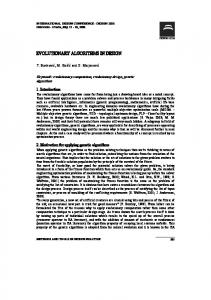
In this section we prove that the emulation procedures presented in Section 6.2 are essentially optimal (i.e. asymptotically and up to a constant factor). Precisely, we prove a lower bound Ω (log n) on the number of slots required to detect collision in some graphs called wheels. A (m, s)-wheel, illustrated in Figure 2, is a graph W = (V, E) such 28

2ms + 2is

.. .

that V = u1 , . . . u4ms , the edges E are all the (ui−1 , ui ) (arithmetic modulo 4ms) plus m spokes, that is edges (uis , u(i+2m)s ) (1 ≤ i ≤ 2m), where the wheel can be odd (all spokes with i odd) or even (all spokes with i even). The even and odd (m, s)-wheels are isomorphic. We consider only situations in which all vertices uis are in the same state, a state in which they wish to beep and all other vertices are in the same internal state, a state in which they do not wish to beep. Thus vertices at the ends of spokes and no others must conclude that there is a collision. We prove that the complexity of any algorithm which detects collision in wheels with high probability is Ω(log n). 4ms

1s

2s

. ..

4s

2ms + 4s

. ..

.. .

2ms + 2s 2ms + 1s 2ms

2is

Fig. 2. A wheel.

Considering a computation of a collision detecting algorithm on a wheel, we define, for any t > 0, bit as the signal (beep or not) from ui to all its neighbours at time t, and, for any t ≥ 0, Bti the sequence bi1 · · · bit . Then, we define the event Et for a spoke uis , u(i+2m)s as follows: o n (i+2m)s−1 (i+2m)s+1 (i+2m)s ) . ) ∧ (Btis−1 = Bt ) ∧ (Btis+1 = Bt Et = (Btis = Bt Lemma 5. For any t (0 ≤ t < s), we have the following: Pr (Et ) ≥ 2−3t . Proof. By induction on t. Clearly the claim is true for t = 0. We suppose that Et−1 is true and we consider probabilities conditional on the values of Bt−1 for is − 1, is, is + 1, (i + 2m)s − 1, (i + 2m)s and (i + 2m)s + 1. (i+2m)s−1 (i+2m)s and = bt and bis−1 We will show that the probability that bis t = bt t (i+2m)s+1 −3 . is at least 2 = b bis+1 t t The three events: (i+2m)s

– bis t = sb (i+2m)s−1 is−1 = bt – bt 29

(i+2m)s+1

– bis+1 = bt t

are independent. For the first, uim and u(i+2m)s started in the same state and have sent and heard identical signals. Thus they have the same probability of beeping at the next round and so have probability at least 1/2 of either both beeping or neither. For the second, the two chains (u(i−1)s · · · uis−1 ) and (u(i+2m−1)s · · · u(i+2m)s−1 ) started in the same states, have received the same signals from uis and u(i+2m)s , and have sent the same signals. Thus, again the two vertices uis−1 and u(i+2m)s−1 have the same conditional probability of beeping and so probability at least 1/2 of making the same choice. The argument for the third event is identical. This proves that the three events happen with probability at least 2−3 yielding that the probability of event Et is lower bounded by 2−3t . ⊔ ⊓ If Et holds for the spoke (uis , u(i+2m)s ), we say that the spoke fails to break symmetry within time t. This happens with probability at least 2−3t and, if it happens, the existence of the spoke has had no influence on the computation up to time t. In particular, whenever uis beeped, u(i+2m)s also beeped and so neither has ever heard the other beep. Theorem 7. For any Monte Carlo algorithm A which detects collision in W , if A halts in less than log2 n/4 rounds with probability greater than 3/4 then for some situations in some wheels, A gives incorrect results for some vertices with probability greater than 1/4. Proof. For simplicity we consider wheels (m, s) where s is a power of 2 and m = 24s−2 /s so that s = log2 n/4. We consider a computation on this wheel without specifying whether it is the odd or even wheel. By the lemma, the probability that a given spoke i breaks symmetry within time s − 1 is at most 1 − 23−3s < exp(−23−3s ) and this is independent for all spokes so that the probability that every spoke breaks symmetry in the even case in time s − 1, is at most exp(−23−3s m) = exp(−2s+1 /s) < 1/4. Hence the probability that the algorithm halts and some spoke fails to break symmetry is greater than 1/2. If, in the even case, spoke i fails to break symmetry, vertex ui hears the same signals from its neighbours in the odd and even cases and, so, if it terminates the algorithm in this time, it has the same probability of deciding collision in the two cases. Hence it gives the wrong response in one case with probability at least 1/2. Hence there is a vertex which gives the wrong response in the odd or even case with probability greater than 1/4. Thus if an algorithm halts in time o(log n) with probability ≥ 3/4, for sufficiently large n it halts in time less than s and so its probability of giving an incorrect result is at least 1/4 for some initial conditions. It follows that the same is true for any algorithm halting in expected time o(log n). ⊔ ⊓ In the context of this paper, we can state explicitly: Corollary 3. The complexity of a Monte Carlo algorithm which detects collision with high probability is Ω(log n). 30

7

Related Work

As explained by Chlebus [12], in a radio network, a node can hear a message only if it was sent by a neighbour and this neighbour was the only neighbour that performed a send operation in that step. If no message has been sent to a node then it hears the background noise. If a node v receives more than one message then we say that a collision occurred at the node v and the node hears the interference noise. If nodes of a network can distinguish the background noise from the interference noise then the network is said to be with collision detection, otherwise it is without collision detection (see for example the Wake-up problem or the MIS problem for radio networks in [19,38,13,26] where nodes do not make the difference between no neighbour sends a message and at least two neighbours send a message; see also the broadcasting problem in radio network in [20] where nodes make the difference between no neighbour sends a message, exactly one neighbour send a message and at least two neighbours send a message). In this context, an efficient randomised emulation of single-hop radio network with collision detection on multi-hop radio network without collision detection is presented and analysed in [5]. To summarise: Remark 7. Detecting a collision in a radio network is to be able to distinguish between 0 message and at least 2 messages while detecting a collision in the beeping model is to be able to distinguish between 1 message and at least 2 messages. Thus, from now on, we consider collisions as explained above for beeping models. Our collision detetection algorithm and the degree computation algorithm use similar ideas to those used for initialising a packet radio network [22] or for election in a complete graph with wireless communications [10] (Algorithm 50, p. 132). The impact of collision detection is studied in [41,30], where it is proved that performances are improved, and in certain cases the improvement can be exponential. The complexity of the conflict resolution problem (the goal is to let every active node use the channel alone (without collision) at least once) is studied in [23] (they assume that nodes are identified), and an efficient deterministic solution is presented and analysed. General considerations and many examples of Las Vegas distributed algorithms related to MIS or colouring can be found in [40]. The computation of a MIS has been the object of extensive research on parallel and distributed complexity in the point to point message passing model [2,35] [3,34]; Karp and Wigderson [27] proved that the MIS problem is in NC. Some links with distributed graph colouring and some recent results on this problem can be found in [33]. The complexity of some special classes of graphs such as growth-bounded graphs is studied in [32]. Results have been obtained also for radio networks [38]. A major contribution is due to Luby [35]. He gives a Las Vegas distributed algorithm. The main idea is to obtain for each node a local total order or a local election which breaks the local symmetry and then each node can decide locally whether it joins the MIS or not. Its time complexity is O(log n) and its bit complexity is O(log2 n). Recently, a Las Vegas distributed algorithm has been presented in [37] which improved the bit complexity: its bit complexity is optimal and equal to O(log n) w.h.p. An experimental comparison between [35] and [37] is presented in [9]. If we remove the 31

constraint on the size of messages or on the anonymity recent new results have been obtained for distributed symmetry breaking (MIS or colouring) in [29,8,6,7]. Afek et al. [1], from considerations concerning the development of certain cells, studied the MIS problem in the discrete beeping model BL as presented in [15]. They consider, in particular, the wake-on-beep model (sleeping nodes wake up upon receiving a beep) and sender-side collision detection Bcd L: they give an O((log n)2 ) rounds MIS algorithm. After this work, Jeavons et al. [24] presents in the model Bcd L a randomised algorithm with feedback mechanism whose expected time to compute a MIS is O(log n). A node v is candidate for joining the independent set (and beeps) with a certain probability (initially 1/2); this value is decreased by some fixed factor if at least one neighbour whishes also to join the independent set. It is increased by the same factor (up to maximum 1/2) if neither v nor any neighbour of v are candidates. More generally, Navlakha and Bar-Joseph present in [39] a general survey on similarities and differences between distributed computations in biological and computational systems and, in this framework, the importance of the beeping model. In the model of point to point message passing, node colouring is mainly studied under two assumptions: - nodes have unique identifiers, and more generally, they have an initial colouring, - every node has the same initial state and initially only knows its own edges. If nodes have an initial colour, Kuhn and Wattenhofer [33] have obtained efficient time complexity algorithms to obtain O(∆) colours in the case where every node can only send its own current colour to all its neighbours. In [25], Johansson analyses a simple randomised distributed node colouring algorithm for anonymous graphs. He proves that this algorithm runs in O(log n) rounds w.h.p. on graphs of size n. The size of each message is log n, thus the bit complexity per channel of this algorithm is O(log2 n). [36] presents an optimal bit and time complexity Las Vegas distributed algorithm for colouring any anonymous graph in O(log n) bit rounds w.h.p. In [15], Cornejo and Kuhn study the interval colouring problem: an interval colouring assigns to each node an interval (contiguous fraction) of resources such that neighbouring nodes do not share resources (it is a variant of node colouring). They assume that each node knows its degree and an upper bound of the maximum degree ∆ of the graph. They present in the beeping model BL a probabilistic algorithm which never stops and stabilises with a correct O(∆)-interval colouring in O(log n) periods w.h.p., where: n is the size of the graph, and a period is Q time slots with Q ≥ ∆, thus it stabilises in O(Q(log n)) slots. Kothapalli et al. consider the family of anonymous rings and show in [28] that if only one bit can be sent along each edge in a round (point to point message passing model), then every Las Vegas distributed node colouring algorithm (in which every node has the same initial state and initially only knows its own edges) needs Ω(log n) rounds w.h.p. to colour the ring of size n with any finite number of colours. Kothapalli et al. consider also√the family of oriented rings and they prove that the bit complexity in this family is Ω( log n) w.h.p. [18] presents and analyses Las Vegas distributed algorithms which compute a MIS or a maximal matching for anonymous rings (in the point to point message passing model). √ Their bit complexity and time complexity are O( log n) w.h.p. 32

Jeavons et al. [24] presents and analyse a colouring algorithm in the message passing model with indistinguishable channels which computes a colouring in O(log n + ∆) slots on average. Emek and Wattenhofer introduce in [17] a model for distributed computations which resembles the beeping model: networked finite state machines (nFSM for short). This model enables the sending of the same message to all neighbours of a node; however it is asynchronous, the states of nodes belong to a finite set, the degree of nodes is bounded and the set of messages is also finite. In the nFSM model they give a 2-hop MIS algorithm for graphs of size n using a set of messages of size 3 with a time complexity equal to O(log n2 ). Model Time (number of Message Information required at number of slots/rounds) size each node colours (bits) Johansson Message O(log n) w.h.p. Ω(log ∆) Distinguishable channels ∆ [25] passing, - own degree point to point M´etivier et Message O(log n + ∆) on aver- O(log µ) Distinguishable channels ∆ al. [36] passing, age and w.h.p. where µ point to equals point max colour used Jeavons et Message O(log n + ∆) on aver- O(log µ) none ∆ al. [24] passing, age where µ equals indistmax inguicolour shable used channels Cornejo et BL never stops stabil- 1 maximum degree ∆ of G O(∆) al. [15] isation w.h.p. in O(∆ log n) This paper Bcd L O(log n + ∆) on aver- 1 none O(log n + ∆) age and w.h.p.
This paper Bcd L O K(log n + log2 K) 1 An upper bound K on K w.h.p. the max degree of G Randomised colouring algorithms on graphs with n vertices; they are all Las Vegas except Cornejo et al. which is Monte Carlo.

References 1. Y. Afek, N. Alon, Z. Bar-Joseph, A. Cornejo, B. Haeupler, and F. Kuhn. Beeping a maximal independent set. Distributed Computing, 26(4):195–208, 2013.

33

2. N. Alon, L. Babai, and A. Itai. A fast and simple randomized parallel algorithm for the maximal independent set. Journal of Algorithms, 7(4):567–583, 1986. 3. B. Awerbuch, A. V. Goldberg, M. Luby, and S. A. Plotkin. Network decomposition and locality in distributed computation. In Proceedings of the 30th ACM Symposium on FOCS, pages 364–369. ACM Press, 1989. 4. K. Azuma. Weighted sums of certain dependent random variables. Tohoku Mathematical Journal, Second Series, 19(3):357–367, 1967. 5. R. Bar-Yehuda, O. Goldreich, and A. Itai. Efficient emulation of single-hop radio network with collision detection on multi-hop radio network with no collision detection. Distributed Computing, 5:67–71, 1991. 6. L. Barenboim and M. Elkin. Distributed Graph Coloring: Fundamentals and Recent Developments. Synthesis Lectures on Distributed Computing Theory. Morgan & Claypool Publishers, 2013. 7. L. Barenboim and M. Elkin. Combinatorial algorithms for distributed graph coloring. Distributed Computing, 27(2):79–93, 2014. 8. L. Barenboim, M. Elkin, S. Pettie, and J. Schneider. The locality of distributed symmetry breaking. In FOCS, pages 321–330, 2012. 9. T. Bisht and K. Kothapalli. An empirical study of two MIS algorithms. In 2013 2nd International Conference on Advanced Computing, Networking and Security, Mangalore, India, December 15-17, 2013, pages 24–28, 2013. 10. Ph. Brandes and R. Wattenhofer. http://disco.ethz.ch/lectures/fs12/podc/lecture/chapter13.pdf. 2012. 11. A. Casteigts, Y. M´etivier, J. Michael Robson, and A. Zemmari. Counting in one-hop beeping networks. CoRR, abs/1605.09516, 2016. 12. B. Chlebus. Randomized communication in radio networks. I:401–456, 2001. 13. M. Chrobak, L. Gasieniec, and D. R. Kowalski. The wake-up problem in multihop radio networks. SIAM J. Comput., 36(5):1453–1471, 2007. 14. J. Collier, N. Monk, P. Maini, and J. Lewis. Pattern formation by lateral inhibition with feedback: a mathematical model of delta-notch intercellular signalling. Journal of Theoretical Biology, 183(4):429–446, 1996. 15. A. Cornejo and F. Kuhn. Deploying wireless networks with beeps. In DISC, pages 148–162, 2010. 16. Y. Emek, Ch. Pfister, J. Seidel, and R. Wattenhofer. Anonymous networks: Randomization = 2-hop coloring. In PODC, 2014. 17. Y. Emek and R. Wattenhofer. Stone age distributed computing. In PODC, pages 137–146, 2013. 18. A. Fontaine, Y. M´etivier, J.-M. Robson, and A. Zemmari. Optimal bit complexity randomized distributed mis and maximal matching algorithms for anonymous rings. Information and Computation, 233:32–40, 2013. 19. L. Gasieniec, A. Pelc, and D. Peleg. The wakeup problem in synchronous broadcast systems. SIAM J. Discrete Math., 14(2):207–222, 2001. 20. M. Ghaffari, B. Haeupler, and M. Khabbazian. Randomized broadcast in radio networks with collision detection. In ACM Symposium on Principles of Distributed Computing, PODC ’13, Montreal, QC, Canada, July 22-24, 2013, pages 325–334, 2013. 21. S. Gilbert and C. Newport. The computational power of beeps. In Proc. of 29th International Symposium on Distributed Computing (DISC), 2015. 22. T. Hayashi, K. Nakano, and S. Olariu. Randomized initialization protocols for packet radio networks. In IPPS/SPDP, pages 544–, 1999. 23. B. Huang and Th. Moscibroda. Conflict resolution and membership problem in beeping channels. In DISC, pages 314–328, 2013. 24. P. Jeavons, A. Scott, and L. Xu. Feedback from nature: simple randomised distributed algorithms for maximal independent set selection and greedy colouring. Distributed Computing, DOI 10.1007/s00446-016-0269-8, 2016. ¨ Johansson. Simple distributed (∆ + 1)-coloring of graphs. Information Processing Letters, 25. O. 70(5):229–232, 1999. 26. T. Jurdzinski and D. R. Kowalski. The wake-up problem in multi-hop radio networks. In Encyclopedia of Algorithms. 2015.

34

27. R. M. Karp and A. Wigderson. A fast parallel algorithm for the maximal independent set problem. In Proceedings of the 16th ACM Symposium on Theory of computing (STOC), pages 266–272. ACM Press, 1984. 28. K. Kothapalli, M. Onus, C. Scheideler, and C. Schindelhauer. Distributed coloring in o/spltilde/(/splradic/(logn)) bit rounds. In 20th International Parallel and Distributed Processing Symposium (IPDPS 2006), Proceedings, 25-29 April 2006, Rhodes Island, Greece. IEEE, 2006. 29. K. Kothapalli and S. V. Pemmaraju. Distributed graph coloring in a few rounds. In PODC, pages 31–40, 2011. 30. D. R. Kowalski and A. Pelc. Leader election in ad hoc radio networks: A keen ear helps. J. Comput. Syst. Sci., 79(7):1164–1180, 2013. 31. S. O. Krumke, M. V. Marathe, and S. S. Ravi. Models and approximation algorithms for channel assignment in radio networks. Wireless Networks, 7(6):575–584, 2001. 32. F. Kuhn, T. Moscibroda, T. Nieberg, and R. Wattenhofer. Fast deterministic distributed maximal independent set computation on growth-bounded graphs. In DISC, pages 273–287, 2005. 33. F. Kuhn and R. Wattenhofer. On the complexity of distributed graph coloring. In Proceedings of the 25 Annual ACM Symposium on Principles of Distributed Computing (PODC), pages 7–15. ACM Press, 2006. 34. N. Linial. Locality in distributed graph algorithms. SIAM J. Comput., 21:193–201, 1992. 35. M. Luby. A simple parallel algorithm for the maximal independent set problem. SIAM J. Comput., 15:1036–1053, 1986. 36. Y. M´etivier, J. M. Robson, N. Saheb-Djahromi, and A. Zemmari. About randomised distributed graph colouring and graph partition algorithms. Inf. Comput., 208(11):1296–1304, 2010. 37. Y. M´etivier, J.-M. Robson, N. Saheb-Djahromi, and A. Zemmari. An optimal bit complexity randomized distributed mis algorithm. Distributed Computing, 23(5-6):331–340, 2011. 38. T. Moscibroda and R. Wattenhofer. Maximal independent set in radio networks. In Proceedings of the 25 Annual ACM Symposium on Principles of Distributed Computing (PODC), pages 148–157. ACM Press, 2005. 39. S. Navlakha and Z. Bar-Joseph. Distributed information processing in biological and computational systems. Commun. ACM, 58(1):94–102, 2015. 40. D. Peleg. Distributed computing - A Locality-sensitive approach. SIAM Monographs on discrete mathematics and applications, 2000. 41. J. Schneider and R. Wattenhofer. What is the use of collision detection (in wireless networks)? In DISC, pages 133–147, 2010. 42. A. Scott, P. Jeavons, and L. Xu. Feedback from nature: an optimal distributed algorithm for maximal independent set selection. In PODC, pages 147–156, 2013.

35