Design, performance, and applications of a coherent ultra-wideband random noise radar Ram M. Narayanan Yi Xu Paul D. Hoffmeyer University of Nebraska—Lincoln Center for Electro-Optics Department of Electrical Engineering Lincoln, Nebraska 68588-0511 E-mail:
[email protected] John O. Curtis U.S. Army Waterways Experiment Station Environmental Laboratory Vicksburg, Mississippi 39180-6199
Abstract. A novel coherent ultra-wideband radar system operating in the 1- to 2-GHz frequency range has been developed recently at the University of Nebraska. The radar system transmits white Gaussian noise. Detection and localization of buried objects is accomplished by correlating the reflected waveform with a time-delayed replica of the transmitted waveform. Broadband dual-polarized log-periodic antennas are used for transmission and reception. A unique signal-processing scheme is used to inject coherence into the system by frequency translation of the ultrawideband signal by a coherent 160-MHz phase-locked source prior to performing heterodyne correlation. The system coherence allows the extraction of a target’s polarimetric amplitude and phase characteristics. This paper describes the unique design features of the radar system, develops the theoretical foundations of noise polarimetry, provides experimental evidence of the polarimetric and resolution capabilities of the system, and demonstrates results obtained in subsurface probing applications. © 1998 Society of Photo-Optical Instrumentation Engineers. [S0091-3286(98)03106-7]
Subject terms: polarimetry; radar; random noise; subsurface probing; ultrawideband. Paper 34097 received Sep. 27, 1997; revised manuscript received Feb. 14, 1998; accepted for publication Feb. 17, 1998.
1
Introduction
Ground-penetrating or subsurface radar systems are increasingly being used for a variety of military and civilian applications.1 Although such systems are essentially similar to other free-space radar systems, they present certain unique problems that demand specialized system design and signal-processing capabilities. Some of the primary issues that need special attention are efficient coupling of the electromagnetic energy into the ground, elimination of the large reflection from the air-ground interface, achieving adequate signal penetration into sometimes lossy media, and achieving adequate signal bandwidth consistent with desired depth resolution. From a phenomenological point of view, factors such as propagation loss, clutter characteristics, and target characteristics are quite different from those in free-space systems. Ground-penetrating radar systems operate over a wide range of probing depths, from closerange high-resolution applications such as locating buried mines and hidden voids in pavements at depths of up to 50 cm, to long-range low-resolution applications, such as probing geologic strata at depths of over 100 m. The University of Nebraska has developed a coherent polarimetric random noise radar system used mainly for detecting shallowly buried minelike objects. This novel ground-penetrating radar ~GPR! system was designed, built, and tested over the last two years. Although the transmit waveform is phase-incoherent, simulation studies and performance tests on the system confirm its ability to respond to phase differences in the received signal. This system uses a wide-bandwidth random noise signal operating within the 1- to 2-GHz frequency range. High spatial resoOpt. Eng. 37(6) 1855–1869 (June 1998)
0091-3286/98/$10.00
lution in the depth ~range! dimension is achieved, due to the wide bandwidth of the transmit signal. The radar system is operated and controlled by a personal computer ~PC!, and the data acquired are stored in the hard drive in real time. From the raw data, the system produces four images corresponding to the copolarized receive amplitude, crosspolarized received amplitude, depolarization ratio, and polarimetric phase difference between the orthogonally polarized received signals. This polarimetric system was used to gather data from a variety of buried targets from a specially designed sandbox 3.5 m long, 1.5 m wide, and 1.0 m deep. Targets that were buried included metallic as well as nonmetallic objects of different sizes and shapes that mimicked land mines as well as other objects. These objects were buried at different depths and with different relative orientations. This paper is organized as follows. Section 2 provides a detailed description of the coherent polarimetric random noise radar system. In Sec. 3, we develop the theoretical foundations of random noise polarimetry. Section 4 describes the results of a simulation study that confirms the ability of the system to respond to phase differences in the reflected signal. In Sec. 5, we show results of proof-ofconcept experimental tests in air that demonstrate the system performance. Section 6 discusses images of buried objects acquired from a specially designed sandbox. Section 7 summarizes and concludes. 2 Radar-System Description A block diagram of the system is shown in Fig. 1. The oscillator OSC1 provides a wideband noise signal with a © 1998 Society of Photo-Optical Instrumentation Engineers 1855
Narayanan et al.: Design, performance, and applications . . .
Fig. 1 Block diagram of polarimetric random noise radar system.
Gaussian amplitude distribution and a constant power spectral density in the 1- to 2-GHz frequency range. The average power output of the noise generator is 0 dBm. This output is split into two in-phase components in the power divider PD1, which has a 1-dB insertion loss over the 3-dB power split. Thus the power divider outputs are at 24-dBm nominal level. One of these outputs is amplified in a power amplifier AMP1, which has a gain of 34 dB and a power output greater than 140 dBm at its 1-dB gain compression point. Thus, the average power output of AMP1 is 130 dBm ~1 W!, but the amplifier is capable of faithfully amplifying noise spikes that can be as high as 10 dB above the mean noise power. The output of the amplifier is connected to a dual-polarized broadband ~1 to 2 GHz! log-periodic transmit antenna ANT1. The antenna, in addition to being broadband, has desirable features such as a frequency-independent gain of 7.5 dB, superior crosspolar isolation greater than 20 dB, and main-to-back lobe ratio better than 30 dB over the operating frequency band. Although our initial design calls for transmission of linearly polarized signals, the dual-polarized antenna can also be configured to transmit circularly polarized signals through the use of switches and hybrids. The other output arm of the power divider PD1 is connected to a combination of a fixed and a variable delay line, DL1 and DL2, respectively. These delay lines are used to provide the necessary time delay for the sampled transmit signal so that it can be correlated with the received signal scattered from objects or interfaces at the appropriate depth corresponding to the delay. The fixed delay line DL1 is used to ensure that the correlation operation is performed only at depths below the air-soil interface, thereby serving to eliminate ground clutter. Since the total probing depths are of the order of 1 m maximum, the delay lines are short, with maximum losses not more than 1 dB. These delay lines are physically realized by low-loss phase shifters, 1856 Optical Engineering, Vol. 37 No. 6, June 1998
which can be rapidly programmed to step through the entire range of available delays, so that various probing depths can be obtained. Assuming a 6-dB maximum loss in DL11DL2, the noise power available at the input of the lower-sideband upconverter MXR1 is 210 dBm. In order to perform coherent processing of the noise signals, a unique frequency translation scheme is proposed. The primary component of this technique is a 160-MHz phase-locked oscillator OSC2, which has a power output of 113 dBm. This is connected via a power divider PD2 to the if input terminal of MXR1. Assuming a 0.5-dB insertion loss in PD2 ~over the 3-dB power split!, an adequate level of 19.5 dBm is available for the frequency translation. The output of MXR1 is the lower sideband of the mixing process, which lies within the 0.84- to 1.84-GHz frequency range. The nominal average power level is 215 dBm. This coherent noise signal is split by power divider PD3 into two channels: the copolarized and the cross-polarized channels. Also, the second output of the power divider PD2 is again split into two 160-MHz signals in the power divider PD4. We now discuss the signal processing of the copolarized channel. The operation in the cross-polarized channel is essentially identical, so it will not be described. One of the outputs of PD3, at a level of 219 dBm, is amplified in a 19-dB-gain amplifier AMP4, thereby providing nominal 0dBm average power at the output. Since this signal is noiselike, the amplifier AMP4 is chosen so as to provide a linear output of 110 dBm minimum. This signal is used as the local oscillator ~LO! input to a biasable mixer MXR2, whose rf input is obtained from the copolarized channel of the receive antenna ANT2 and a 20-dB-gain low-noise amplifier AMP2. The receive antenna is identical to the transmit antenna. Amplifier AMP2 is used to improve the noise figure at the receiver input. The mixer MXR2 is biased in the square-law region using a dc voltage, since the LO drive, being of varying amplitude, can sometimes attain low power levels, resulting in an inefficient mixing process. The dc bias ensures that the mixing process is efficient for LO drive levels as low as 210 dBm. In general, the rf input signal to the mixer MXR2 consists of transmitted noise at 1 to 2 GHz scattered and reflected from various objects/interfaces. However, since the LO signal has a unique delay associated with it, only the signal scattered from the appropriate depth ~i.e., range! bin will mix with the LO to yield an if signal at a frequency of exactly 160 MHz. The output of the mixer MXR2 is connected to a narrow-band bandpass filter FL1 of center frequency 160 MHz and bandwidth 5 MHz, ensuring that only 160-MHz signals get through. The output of the filter FL1 at 160 MHz is split into two outputs in the power divider PD5. One of these outputs is amplified and detected in a 70-dBdynamic-range 160-MHz logarithmic amplifier AMP6, whose logarithmic transfer function was measured as 25.2 mV/dB. The wide dynamic range ensures that a wide range of scattered power levels can be processed. The other output of the power divider PD5 is connected to one of the inputs of an I/Q detector IQD1, whose reference input is one of the outputs from PD4. Both of the signals are exactly at 160 MHz; thus the I/Q detector provides the inphase ~I! and quadrature ~Q! components of the phase dif-
Narayanan et al.: Design, performance, and applications . . .
ference between the two signals. Since frequency translation preserves phase differences, the I and Q outputs can be related to the polarimetric copolarized scattering characteristics of the buried object or interface. In a similar fashion, the cross-polarized channel is simultaneously processed using an amplifier AMP5 ~equivalent to AMP4!, biasable mixer MXR3 ~equivalent to MXR2!, 160-MHz bandpass filter FL1 ~equivalent to FL2!, power divider PD5 ~equivalent to PD6!, logarithmic amplifier AMP7 ~equivalent to AMP6!, and I/Q detector IQD2 ~equivalent to IQD1!. The system therefore produces the following outputs at various depths as set by the delay lines: 1. 2. 3. 4.
copolarized amplitude copolarized phase angle cross-polarized amplitude cross-polarized phase angle.
Photographs of the polarimetric random noise radar system are shown in Fig. 2. 3
Theory of Random Noise Polarimetry
Since the transmitted signal has a random amplitude distribution and a uniform power spectral density, we model the transmit voltage wave v t (t) as v t ~ t ! 5a ~ t ! cos~ v 0 1 d v ! t,
~1!
where a(t) takes into account the amplitude distribution, d v (t) takes into account the frequency spectrum of v t (t), and v 0 is the center frequency of transmission. We assume that a(t) follows a Gaussian distribution while d v (t) follows a uniform distribution, and that both a(t) and d v (t) are ergodic processes. Furthermore, we assume that a(t) and d v (t) are uncorrelated and statistically independent. The average power transmitted, P t , is given by P t5
v 2t ~ t !
R0
,
~2! Fig. 2 Photographs of polarimetric random noise radar system.
where R 0 is the characteristic system impedance, and a bar over a variable denotes its time-average value. Since a(t) and d v (t) are independent, we can write v 2t ~ t ! 5a 2 ~ t ! cos2 $ ~ v 0 1 d v ! t %
5a 2 ~ t ! • cos2 $ @ v 0 1 d v ~ t !# t % 5
1 2
a 2~ t ! ,
object reflectivity are invariant with frequency. If the dielectric constant of soil is e r (5 e r8 2 j e r9 ), the phase velocity of the electromagnetic wave is v p5
~4!
if we assume that the soil medium is low-loss, i.e., e r9 ! e r8 . Thus, the two-way delay for a signal that is transmitted, reflected, and arriving at the receive antenna, t, is
since the average value of cos2(•) is 1/2. Thus, P t5
1 a 2~ t ! . 2R 0
c
~3!
Consider an object of complex reflectivity R exp(jf0) buried at a depth d. To simplify the analysis, we assume that both the magnitude R and the phase angle f 0 of the
t5
~5!
Ae r8
2d 2d Ae r8 . 5 c vp
~6!
Optical Engineering, Vol. 37 No. 6, June 1998 1857
Narayanan et al.: Design, performance, and applications . . .
For lossy media, the phase velocity v p is lower than in the lossless case, thereby increasing the two-way signal delay t. Let the propagation constant in soil, g, be given by
g5a1 jb
~7!
Since both of these signals are at the same frequency v 8 , the I/Q detector can unambiguously measure the phase difference u, given by
u ~ t ! 52 v 8 t 1 f 0 22 b d.
~16!
The average value of u as measured by the I/Q detector is
where a is the attenuation constant and b is the phase constant. In general, a and b both increase with frequency. Thus, the two-way propagation factor is given by
¯u 52 v 8 t 1 f 0 22 b d.
A ~ d ! 5exp~ 22 g d !
Note that ¯b is simply the value of b at v 5 v 0 , which is
5exp~ 22 a d ! exp~ 22 j b d ! .
~8!
The time-varying expression for the received voltage v r (t) can now be obtained as the time-delayed version of v t (t) modified to include the effects of scattering and twoway propagation: v r ~ t ! 5a ~ t2 t ! R exp~ 22 a d ! cos@~ v 0 1 d v !~ t2 t ! 1 f 0
22 b d # .
~9!
The time-delayed sample of the transmit signal is v t ~ t2 t ! 5a ~ t2 t ! cos@~ v 0 1 d v !~ t2 t !# .
~10!
When this signal is passed through a double-sideband upconverter whose if is v 8 , the lower-sideband output v 8t (t 2 t ) is v t8 ~ t2 t ! 5a ~ t2 t ! cos@~ v 0 2 v 8 1 d v !~ t2 t !# .
~11!
The difference frequency from the mixing of v r (t) and v 8t (t2 t ) yields a voltage v d (t) given by v d ~ t ! 5K 1 Ra 2 ~ t2 t ! exp~ 22 a d ! cos@ v 8 ~ t2 t ! 1 f 0
22 b d # ,
~12!
¯b 5
v 0 Ae r8 . c
~18!
We therefore obtain ¯u 5 f 0 2 v 8 t 2
2 v 0 Ae r8 d c
~20!
P rx 5K 2 R 2x .
~21!
Thus the ratio of P rx to P rc yields the power depolarization ratio D, which is seen to be independent of the system transfer function, i.e.,
V d 5K 1 Ra 2 ~ t2 t ! exp~ 22 a 0 d !
Furthermore, we have
where a 0 is the value of a at v 5 v 0 . The average power in this signal, P r , is given by V d2 52K 21 R 0 P 2t exp~ 24 a 0 d ! R 2 5K 2 R 2 , P r5 2R 0
where K 2 is a constant. Thus measurement of the power P r yields the square of the reflection coefficient magnitude. In order to measure the phase f 0 , consider the output of the I/Q detector fed by v d (t) and v 1 (t), where v 1 (t) is given by v 1 ~ t ! 5cos v 8 t. 1858 Optical Engineering, Vol. 37 No. 6, June 1998
u c 5 f 0c 2 v 8 t 22 b d
~15!
~22!
~23!
and
u x 5 f 0x 2 v 8 t 22 b d. ~14!
~19!
P rc 5K 2 R 2c ,
P rx R 2x 5 5D. P rc R 2c
~13!
.
Thus, a measurement of the average value of u yields the phase angle f 0 . Until this point, we have not considered the effects of polarization. If the antenna can simultaneously measure both the copolarized and the cross-polarized scattered power, and if the hardware for copolarized and crosspolarized channels is identical, then we can measure P rc , P rx , u c , and u x , where the subscripts c and x refer to the copolarized and the cross-polarized channels, respectively. Thus
where K 1 is some constant. Note that this signal is always centered around v 8 . The average amplitude of this signal, V d , is given by
52K 1 RR 0 P t exp~ 22 a 0 d ! ,
~17!
~24!
Thus the difference between u x and u c yields the phase angle between the cross-polarized and copolarized channels, again seen to be independent of the system:
u x 2 u c 5 f 0x 2 f 0c .
~25!
The resolution properties of the system can be easily observed by considering a received signal from another range ~or depth! bin whose delay is different from t. Let the
Narayanan et al.: Design, performance, and applications . . .
delay from the buried object be t 8 , but the delay within the system be t. In this case, v r (t) is now modified and expressed as v r8 (t) as follows: v r8 ~ t ! 5a ~ t2 t 8 ! exp~ 22 a d ! cos@~ v 0 1 d v 8 !~ t2 t 8 ! 1 f 0
22 b d # .
~26!
When this signal is mixed with v 8t (t2 t ), we get v 8d (t) given by v 8d ~ t ! 5Ra ~ t2 t ! a ~ t2 t 8 ! exp$ 22 a d % cos@ v 8 ~ t2 t !
2 v 0 ~ t2 t 8 ! 1 d v 8 ~ t2 t 8 ! 2 d v ~ t2 t ! 1 f 0 22 b d # .
~27!
Since the noise voltage a(t) has a temporal correlation function of the form (sin x)/x, we have the result a ~ t 1 ! a ~ t 2 ! 50
~28!
for u t 1 2t 2 u @1/B, where B is the system bandwidth. Thus, the average power in the signal v 8d (t) can be shown to be equal to zero. We see, therefore, that unless the internal time delay is exactly matched to the expected time delay, the output of the detector is zero. As we step the internal time delay t from zero to the maximum expected value, the depth profile of scattering can be built up by the system, so that not only can targets be identified, but they can also be localized. In practice, the practical system will suffer from drawbacks such as system nonlinearities in amplitude and phase that can degrade the detection efficiency and resolution. In an ideal case, the resolution is determined by the system bandwidth B. The resolution Dd is given by Dd5
c vp 5 . 2B 2 Ae r8 B
~29!
For c533108 m/s and B51 GHz, we get Dd5
15
Ae r8
cm.
~30!
For dry soil, e r8 '3, and for wet soil, e r8 '25. Thus the system resolution varies from 8.6 cm in dry soil to 3 cm in wet soil, with an average value of about 5 cm. The maximum depth of detection is limited by the noise figure of the front end-receiver amplifier and the loss characteristics of the soil. The noise power level at the receiver, N, is given by N5kTB D F,
~31!
where k is the Boltzmann constant (1.37310223 J/K), T is the ambient temperature ~assumed to be 300 K!, B D is the detection bandwidth ~5 MHz!, and F is the front-end amplifier noise figure (2 dB51.58). Using these values, the noise power at the receiver is computed as 2104.9 dBm.
Soil losses vary widely in value, ranging from about 1–2 dB/m for dry sand to over 100 dB/m for wet clay, thereby yielding widely varying detection depths depending upon soil type and moisture content. It must also be noted that the transmission coefficient at the air-soil interface is modified by scattering caused by the soil surface roughness, although this effect is not expected to be significant, owing to the lower frequencies used for subsurface probing. From the raw data collected by the radar system, we generate images based on the Stokes matrix formulation for facilitating the detection and recognition of targets using the polarimetric information on the buried target. The Stokes vector is a convenient method for representing the polarization state of an electromagnetic wave. It is denoted as S and given by
FG
S0 S1 , S5 S2 S3
~32!
where the individual elements are defined as follows: S 05 u E Hu 21 u E Vu 2,
~33!
S 15 u E Hu 22 u E Vu 2,
~34!
S 2 52 u E H uu E V u cos u d ,
~35!
S 3 52 u E H uu E V u sin u d .
~36!
In the above equations, u d is the polarimetric phase angle, i.e., the difference between the phase angles of the horizontally received signal and the vertically received signal. Also, u E H u and u E V u are the electric field amplitudes of the horizontally and vertically polarized received signals, whose squared values represent the copolarized reflected power and cross-polarized reflected power, respectively ~assuming the transmit polarization is horizontal!. We recognize S 0 as the total reflected power ~sum of the copolarized and the cross-polarized reflected power!. Likewise, S 1 is the difference between the copolarized and the crosspolarized reflected power. Finally, S 2 is proportional to the cosine of the polarimetric phase angle u d , while S 3 is proportional to its sine. Both S 2 and S 3 are weighted by the absolute electric field amplitudes of the reflected copolarized and cross-polarized signals, as can be seen from their definitions. It is also to be noted that S 20 5S 21 1S 22 1S 23 .
~37!
The use of S 2 and S 3 is very helpful in detecting targets, since these parameters move in opposite directions and thereby provide additional information about the reflected signal. When S 2 is high, S 3 is low, and vice versa. Thus, no matter what the polarimetric phase angle is, the target image is bound to show up in either S 2 or S 3 , and sometimes in both. Optical Engineering, Vol. 37 No. 6, June 1998 1859
Narayanan et al.: Design, performance, and applications . . .
Fig. 3 Simulation results using random noise waveform for target reflectivity of 1 exp(j 0): (a) transmitted signal amplitude versus time, (b) transmitted signal shifted by 6 v 8 to simulate the doublesideband upconversion, (c) received signal amplitude versus time after two-way propagation and reflection, (d) multiplied output of signals in (b) and (c) versus time, (e) spectrum of filtered output in (d), showing the peak at v 8 , and (f) multiplied output in (d) filtered at v 8 , showing the input signal at the I/Q detector versus time (solid line).
4 Results of Simulation Study Various computer simulations were performed to evaluate the performance of the radar system design.2 These simulations were performed for various combinations of soil type, soil moisture, depth of target burial, and polarimetric response of the buried target. Ground reflections as well as uncorrelated system noise were added to the received signal to simulate realistic field conditions. Results of simulations using random noise as the probing signal are shown in Figs. 3 and 4. In Fig. 3, the reflectivity of the buried object is assumed to be 1 exp(j0), while in Fig. 4 it is assumed to be 1 exp(jp/2). The objects are assumed to be located at a 1860 Optical Engineering, Vol. 37 No. 6, June 1998
depth of 5 cm in clayey soil ~48% clay, 40% silt! with 10% volumetric moisture, whose dielectric constant was computed as e r 54.562 j1.32. The following plots are shown in the figures: ~a! transmitted signal amplitude versus time ~b! transmitted signal shifted by 6 v 8 to simulate the double-sideband upconversion ~c! received signal amplitude versus time after two-way propagation and reflection
Narayanan et al.: Design, performance, and applications . . .
Fig. 4 Simulation results using random noise waveform for target reflectivity of 1 exp(jp/2): (a) transmitted signal amplitude versus time, (b) transmitted signal shifted by 6 v 8 to simulate the doublesideband upconversion, (c) received signal amplitude versus time after two-way propagation and reflection, (d) multiplied output of signals in (b) and (c) versus time, (e) spectrum of filtered output in (d), showing the peak at v 8 , and (f) multiplied output in (d) filtered at v 8 , showing the input signal at the I/Q detector versus time (solid line).
~d! multiplied output of signals in ~b! and ~c! versus time ~e! spectrum of filtered output in ~d!, showing the peak at v 8 ~f! multiplied output in ~d! filtered at v 8 , showing the input signal at the I/Q detector versus time ~solid line!.
As can be seen, the polarimetric phase of the reflection from the buried object is clearly evident in Figs. 3~f! and 4~f!. These signals are 90 deg out of phase, consistent with the 90-deg phase difference in their assumed reflectivity. Results of simulations using a spread-spectrum waveform as the probing signal are shown in Fig. 5. The transmitted signal was assumed to be of constant amplitude 1, Optical Engineering, Vol. 37 No. 6, June 1998 1861
Narayanan et al.: Design, performance, and applications . . .
Fig. 5 Simulation results using spread-spectrum waveform for target reflectivity of 1 exp(j 0): (a) transmitted signal amplitude versus time, (b) transmitted signal shifted by 6 v 8 to simulate the doublesideband upconversion, (c) received signal amplitude versus time after two-way propagation and reflection, (d) multiplied output of signals in (b) and (c) versus time, (e) spectrum of filtered output in (d), showing the peak at v 8 , and (f) multiplied output in (d) filtered at v 8 , showing the input signal at the I/Q detector versus time (solid line).
while its frequency was changed in a random fashion between 1 and 2 GHz after each burst. The target reflectivity was assumed to be 1 exp(j0), while the soil and depth parameters were kept the same. Comparison of Figs. 3~f! and 5~f! indicates that the phase of the reflected signal is indeed preserved, and is independent of the transmitted waveform type. We also confirmed that the ratio of the power received to that transmitted, i.e., the average power in ~f! divided by average power in ~a!, was the same for both types of waveforms considered. 1862 Optical Engineering, Vol. 37 No. 6, June 1998
5
Proof-of-Concept Experimental Results
Preliminary test results on the radar system in air confirm its ability to extract the polarimetric response of targets with good range or depth resolution.3 These results are in conformity with our simulation studies performed earlier and described above. Figure 6 shows the ability of the system to track reflected signals from targets at various ranges. In this experiment, the transmitter output was directly connected to the copolarized receiver input using a coaxial cable, effectively
Narayanan et al.: Design, performance, and applications . . .
Fig. 7 Change in detected phase of copolarized signal as a function of incremental target range.
Fig. 6 Copolarized signal amplitude as a function of system delay under direct transmitter-receiver connection at various cable lengths.
bypassing both antennas. The intention was to confirm if the system delay time, as set by the variable delay line DL2, was able to track the pseudoreflected signal as its range was varied. The top curve shows a plot of the copolarized amplitude as a function of the system delay time for a coaxial-cable length of 1 m, which shows that the peak occurs at a delay time of 6 ns. The bottom curve shows that the peak occurs at a delay time of 10 ns for a cable length of 1.7 m. Using these values, the dielectric constant of the coaxial cable is computed as 2.9, which agrees with the manufacturer’s specification of 2.8. Thus, the radar system is capable of tracking reflections from targets by observing the delay time of the peak signal amplitude. Figure 6 also reveals that the cross-correlation function approximates the typical (sin x)/x response for the voltage with a sidelobe level of 13 dB. Thus, the maximum sidelobe level for power, which is proportional to the square of the voltage, is 26 dB. We note from Fig. 6 that an amplitude difference of approximately 600 mV exists between the peak of the correlation function and the sidelobes for the detected voltage. This corresponds to a sidelobe level of 23.8 dB for the reflected power, since the transfer function of the logarithmic amplifier is 25.2 mV/dB. Thus, the response from adjacent depth bins will obscure the main-lobe target response only if the reflectivity of the target located in the adjacent bin is about 24 dB higher than that of the main-lobe target.
The ability of the system to track the phase of the reflected signal amplitude was also confirmed. The radar system was pointed at a metal plate at a range of 1.2 m, and the phase of the copolarized signal, ¯ u c , was measured from the outputs of the I/Q detector IQD1. The metal plate was then moved back in 15-cm increments, and the corresponding unwrapped phase angle measured. A plot of the phaseangle difference ~from the 1.2-m reference! as a function of the range increment is seen to be linear in Fig. 7, thus showing that the system does respond to controlled phase changes brought about by changes in the transit time between the transmit and receive signals. In order to observe the polarimetric response of the radar system, a polarizing grid was fabricated. This was a square 60 cm360 cm wooden frame inside which thick copper wires were fixed along one direction at 5-cm spacing. The grid was placed in front of the antennas with the longitudinal axes of the copper wires parallel to the transmit electric field vector. This was denoted as u 590 deg. The depolarization ratio D was measured for different values of the angle between the polarizing grid axis and the electric field vector by rotating the grid, and this is plotted in Fig. 8. As expected, the D value is minimum when the axis of the grid coincides with the electric field vector, and reaches a value of 1 when the angle u is 45 deg. Below 45 deg, both copo-
Fig. 8 Depolarization ratio as a function of the angle between the electric field vector and the longitudinal polarizing grid axis. Optical Engineering, Vol. 37 No. 6, June 1998 1863
Narayanan et al.: Design, performance, and applications . . .
larized and cross-polarized signal amplitudes are very low, and this results in the D value leveling off to about 1. Finally, the resolution capabilities of the system were confirmed to meet design specifications. Since the system bandwidth is 1 GHz, the theoretical resolution in air is 15 cm. To test this, two similar objects were placed side by side within the antenna beams. The copolarized signal amplitude was recorded for three different distances between the objects ~one object was kept fixed, while the other was moved back in 7.5-cm increments!. These results are shown in Fig. 9. The dot-dash line is the raw data, while the solid line shows the smoothed data. When the target separation is zero, there is one single peak observed near the 9-ns delay time. At 7.5-cm separation, only one target is observed at 9 ns, but the peak appears somewhat broader. At 15-cm separation, we clearly see the presence of two discernible wellresolved peaks. Thus, our proof-of-concept experimental results do confirm that this novel radar system has the ability to characterize the high-resolution polarimetric scattering response of targets in air. 6 Results of Field Tests The radar system was used to gather data from an assortment of different buried objects in a specially designed sandbox.4 The sandbox is 3.5 m long, 1.5 m wide, and 1 m deep. Metallic as well as nonmetallic objects were buried at different depths and orientations. The radar antennas were scanned over the surface as data were collected continuously. The operational configuration is with the antennas pointing down; hence leakage through backlobes is not expected to be a problem, unless highly reflective objects appear above the system as it is scanned. Photographs of the data collection setup are shown in Fig. 10.
Raw Images The following raw images were obtained using the polarimetric random noise radar. Each figure ~Figs. 11–14! contains four images from one radar scan over various buried objects. The top image is the copolarized received power. The second image is the cross-polarized received power. The third image is the depolarization ratio, and the fourth image is the absolute phase difference between the copolarized and the cross-polarized received channels. The relative amplitude scale in decibels applies to the copolarized and cross-polarized power, and the depolarization ratio. Figure 11 shows the image pertaining to two metal plates, each 23 cm in diameter and 2 cm in thickness, buried 23 cm below the surface with a 30-cm lateral separation between the two. The copolarized and depolarization-ratio images clearly show and resolve these two objects. Figure 12 is the image obtained from the same metal plates as in Fig. 11, but with each plate buried at different depths. The first was buried 23 cm below the surface, and the second at 8 cm. The spacing between the plates was changed to 15 cm. Again the copolarized and depolarization-ratio images not only clearly show these objects, but are also able to resolve them. Figure 13 shows the image pertaining to a metal plate ~same size and shape as above! and an identical wooden plate. Both plates were buried at a depth of 23 cm below the surface, with a lateral separation of 30 cm. In this im6.1
1864 Optical Engineering, Vol. 37 No. 6, June 1998
Fig. 9 Copolarized signal amplitude as a function of system delay time for various separations between identical targets.
Narayanan et al.: Design, performance, and applications . . .
Fig. 10 Photographs of test setup showing data collection.
age, it is easy to detect the metal plate, but the wooden plate is not clearly observable on account of its low dielectric contrast with respect to the soil medium. Further data processing using the phase information may make this object more visible, and one such technique based on Stokes matrix processing is discussed in the next subsection. Figure 14 shows the image of a 6-cm-diam metal pipe that was buried 29 cm below the surface. The transmit polarization was parallel to the pipe’s axis, and the scan direction was perpendicular to the pipe’s axis. Under these conditions, the pipe acts as a point target with low interaction time with the radar during its scan. Again the copolarized and depolarization-ratio images clearly show the pipe, and the familiar hyperbolic curve shape is observed. From the images shown, it is easy to conclude that metallic objects are fairly easy to locate with the polarimetric random noise radar. Nonmetallic objects, such as the
Fig. 11 Raw image of two metal plates buried at same depth: (a) copolarized received power, (b) cross-polarized received power, (c) depolarization ratio, and (d) polarimetric phase difference.
wooden plate, are much harder to discern from the raw data, and additional processing may be required in order to enhance detection. The initial large reflection from the surface also obscures objects just below the surface. Further signal processing may also be used to overcome this drawback. The next subsection describes results from Stokes matrix processing. 6.2 Processed Images Stokes matrix images were generated and combined with simple image-processing operations to improve target deOptical Engineering, Vol. 37 No. 6, June 1998 1865
Narayanan et al.: Design, performance, and applications . . .
Fig. 12 Raw image of two metal plates buried at different depths: (a) copolarized received power, (b) cross-polarized received power, (c) depolarization ratio, and (d) polarimetric phase difference.
Fig. 13 Raw image of a metal plate and a wooden plate buried at same depth: (a) copolarized received power, (b) cross-polarized received power, (c) depolarization ratio, and (d) polarimetric phase difference.
tectability and clutter rejection. The smoothing filter is used for reduction of radar clutter and noise. It was found from the original raw data that high-frequency tonal variations were prevalent in regions without targets, and these grainy variations were attributed to the fact that the soil volume was inhomogeneous, and contained voids and rocks. The smoothing operation, when performed, results in low-pass filtering and eliminates the high-frequency noise components. The thresholding operation is applied on the global
scale to the entire smoothed image. It enhances image intensities above the mean intensity of the entire image, thereby enhancing target detectability, while simultaneously eliminating clutter, identified as low-intensity areas, by setting these to zero digital number. As will be shown, these postprocessing operations are successful in reducing clutter and enhancing target detectability. We emphasize here that smoothing and thresholding operations
1866 Optical Engineering, Vol. 37 No. 6, June 1998
Narayanan et al.: Design, performance, and applications . . .
Fig. 15 Postprocessed (smoothed and thresholded) images of a metal plate and a wooden plate buried at same depth: (a) S 0 , (b) S 1 , (c) S 2 , and (d) S 3 .
Fig. 14 Raw image of metal pipe with axis parallel to transmit polarization and perpendicular to scan direction: (a) copolarized received power, (b) cross-polarized received power, (c) depolarization ratio, and (d) polarimetric phase difference.
were performed on all four Stokes matrix images. The relative amplitude scale in decibels applies to all four images. The three postprocessed images ~Figs. 15–17! show S 0 ~top left!, S 1 ~bottom left!, S 2 ~top right!, and S 3 ~bottom right!. The preprocessed image corresponding to two objects, one a round metal plate 23 cm in diameter and 2 cm thick, and the other a wooden plate of the same shape and dimensions, is shown in Fig. 13. The objects are both bur-
ied in dry sand at 23-cm depth, with a lateral separation of 23 cm. The Stokes matrix processed images are shown in Fig. 15. Both objects, especially the wooden plate ~right object! are detectable in the S 1 image. In Fig. 16 and Fig. 17, we also show images of polarization-sensitive objects to demonstrate the ability of the system to utilize polarimetric features of the target. In these figures, images were obtained for combinations of target orientation parallel to ~Fig. 16! and perpendicular to ~Fig. 17! the scan direction. Note that Fig. 17 is the postprocessed image whose raw version is shown in Fig. 14. The transmit polarization was parallel to the longitudinal axis of the object, which was a metal pipe 6 cm in diameter and 85 cm long. When the transmit polarization was perOptical Engineering, Vol. 37 No. 6, June 1998 1867
Narayanan et al.: Design, performance, and applications . . .
Fig. 16 Postprocessed (smoothed and thresholded) images of a metal pipe with axis parallel to transmit polarization and parallel to scan direction: (a) S 0 , (b) S 1 , (c) S 2 , and (d) S 3 .
Fig. 17 Postprocessed (smoothed and thresholded) images of a metal pipe with axis parallel to transmit polarization and perpendicular to scan direction: (a) S 0 , (b) S 1 , (c) S 2 , and (d) S 3 .
pendicular to the object axis, detection was not possible; hence, these images are not shown. From the processed images, we observe that a long slender object can be detected, no matter what its orientation is with respect to the scan direction, as long as the transmit polarization is parallel to the object orientation. This indicates that a dualpolarized transmitter, i.e., one that simultaneously or switchably transmits vertically and horizontally polarized signals, can easily detect such an object.
a powerful technique for obtaining high-resolution images. Other applications being investigated that exploit the coherence in the system include interferometric ~using spaced antennas! and synthetic aperture radar ~SAR! techniques to sharpen the azimuthal resolution. In addition, random noise polarimetry can be used in foliage penetration ~FOPEN! radar systems by operating at lower frequencies, typically in the 250- to 500-MHz frequency range.
7 Conclusions In this paper, we have demonstrated the potential of random noise polarimetry for high-resolution subsurface probing applications. This unique concept synergistically combines the advantages of a random noise ultra-wideband waveform with the power of coherent processing to provide 1868 Optical Engineering, Vol. 37 No. 6, June 1998
Acknowledgments This work was supported by the U.S. Army Waterways Experiment Station through contract DACA39-93-K-0031. We appreciate the assistance of Dr. Lim Nguyen, who provided valuable comments.
Narayanan et al.: Design, performance, and applications . . .
References 1. D. J. Daniels, D. J. Gunton, and H. F. Scott, ‘‘Introduction to subsurface radar,’’ IEE Proc. F 135, 278–320 ~Aug. 1988!. 2. R. M. Narayanan, Y. Xu, and D. W. Rhoades, ‘‘Simulation of a polarimetric random noise/spread spectrum radar for subsurface probing applications,’’ in Proc. IGARSS’94 Symp., IEEE, pp. 2494–2498, Pasadena ~Aug. 1994!. 3. R. M. Narayanan, Y. Xu, P. D. Hoffmeyer, and J. O. Curtis, ‘‘Design and performance of a polarimetric random noise radar for detection of shallow buried targets,’’ in Detection Technologies for Mines and Minelike Targets, Proc. SPIE Orlando, 2496, 20–30 ~Apr. 1995!. 4. R. M. Narayanan, Y. Xu, P. D. Hoffmeyer, and J. O. Curtis, ‘‘Random noise polarimetry applications to subsurface probing,’’ Detection and Remediation Technologies for Mines and Minelike Targets, Proc. SPIE Orlando, 2765, 360–370 ~Apr. 1996!. Ram M. Narayanan received his BTech degree from the Indian Institute of Technology, Madras, India, in 1976, and his PhD degree from the University of Massachusetts, Amherst, MA, in 1988, both in electrical engineering. From 1976 to 1983, Dr. Narayanan was employed as a research and development engineer at Bharat Electronics Ltd., Ghaziabad, India, where he was involved in the development of microwave troposcatter communications equipment for the Indian Army and Air Force. He joined the Microwave Remote Sensing Laboratory at the University of Massachusetts, Amherst, MA, in 1983. His doctoral dissertation was on millimeter-wave scattering from vegetation and snow. He joined the University of Nebraska-Lincoln in 1988, where he is currently associate professor of electrical engineering. Dr. Narayanan’s research interests lie in the area of radar and laser remote sensing, and the development of ultrawideband radar systems. He serves on the IEEE Geoscience and Remote Sensing Society Administrative Committee, and on the National Research Council Committee on Radio Frequencies. Yi Xu received the BS degree from Beijing Normal University, Beijing, P.R. China, in 1982, the MS degree from Hangzhou University, Hangzhou, P.R. China, in 1989, and the PhD degree from University of Nebraska-Lincoln in 1997, all in electrical engineering. His doctoral dissertation dealt with the development of the random noise polarimetry technique for subsurface probing applications. Dr. Xu’s main areas of research interest are groundpenetrating radar system design and applications, remote sensing,
signal and image processing, and data communication and computer programming. He is currently with Sitel Corporation, Omaha, Nebraska. Paul D. Hoffmeyer received his BS degree in electrical engineering from the University of Nebraska, Lincoln, in 1994. He is currently pursuing his MS degree in electrical engineering at the University of Nebraska-Lincoln. In 1997, he joined Telex Communications in Lincoln, Nebraska, as an antenna design engineer.
John O. Curtis received his BSME degree with high honor from Northeastern University, Boston, MA, in 1971, the MS degree in engineering mechanics from Colorado State University, Fort Collins, in 1973, and his PhD degree in physics from Dartmouth College, Hanover, NH, in 1992. Dr. Curtis has served the Army research and development community as both a researcher and a project manager. His early assignments dealt with dynamic finite element simulations of the soil-structure interaction problems that included the development of non-linear constitutive models for soils. He then became involved in measuring and modeling the thermal infrared signatures of the Army’s high-valued fixed facilities and in better understanding as to how to protect these facilities against air-to-ground threats from sophisticated weapon systems and their users. His most recent work focuses directly on some of the issues relevant to subsurface characterization of military sites. Among these are measurements of the complex dielectric properties of soils and attempts to understand how soil moisture, sample density, sample chemistry, and other factors play a part in controlling the dielectric properties of soils. The goal of this research is to generate tools that will allow the designer to better predict the speed and losses associated with electromagnetic propagation through soils under a variety of environmental conditions.
Optical Engineering, Vol. 37 No. 6, June 1998 1869