Design Space Exploration of Caches Using Compressed Traces

Design Space Exploration of Caches Using Compressed Traces Xianfeng Li [email protected]

Hemendra Singh Negi [email protected]

Tulika Mitra [email protected]

Abhik Roychoudhury [email protected]

School of Computing National University of Singapore Republic of Singapore 117543

ABSTRACT

1.

Memory subsystem, in particular, cache design is important for both high performance and embedded computing systems. The trend towards increased customization for embedded systems, in addition, requires the design of an optimal cache configuration for each application. Trace driven simulation is widely used to evaluate cache performance. However, traces are storage inefficient and simulation is too slow especially when hundreds of design points need to be evaluated. Trace based simulation has two sources of redundancies: multiple occurrences of the same sequence in the trace and containment relationship among cache configurations. We exploit both the redundancies in a unified manner by simulating multiple cache configurations in a single pass directly over a compressed trace (which has already identified the repetitive sequences). Experimental results indicate that our approach achieves significant savings both in storage and in simulation time compared to existing methods.

Memory subsystems, and in particular caches, have significant impact on performance, power, and size of both high performance and embedded computing systems. For high performance systems, the processor architect attempts to find the optimal memory subsystem given a set of representative applications expected to run on the system. An embedded system, on the other hand, runs a specific application program for the entire lifetime of the system. As the application program is fixed, there exists a lot of flexibility in choosing an optimal design for the application in question. In particular, customized processors [4, 6] and configurable system-on-chip platforms [1] provide the designer of an embedded system with the opportunity to configure the memory subsystem for a particular application. This brings us to the problem of design space exploration: the designer needs to explore the various choices efficiently for a given application program. In this paper, we concentrate on choosing a suitable data/instruction cache for a given application program, where some representative inputs are provided by the user. The problem of design space exploration is computationally intensive. Clearly, it is expensive to simulate the traces for the representative inputs over the space of all designs. Consider the task of deciding a suitable cache memory for a given application. The design of the cache memory involves instantiating several parameters: line size, number of lines, associativity, replacement policy etc. Thus, the number of possible cache memories to be tried out can easily grow to hundreds. In addition, the traces of realistic programs can grow to billions of instructions. Clearly it is infeasible (both in time and space) to do a naive simulation of such traces on all possible design points. One possible approach to solve this problem would be to ignore part of the design space by applying statistical techniques. An alternative approach would be to identify and avoid the redundancies in the computation involved in exhaustive design space exploration. In this paper, we have taken the second approach. Given a representative trace of an application program, we employ a time and space efficient strategy to find out the optimal cache configuration for the trace. Note that with the increasing processor-memory gap, reducing the number of

Categories and Subject Descriptors B.3.2 [Memory Structures]: Design Styles—Cache memories

General Terms Algorithms, Performance, Design.

Keywords Cache, single pass simulation, compressed trace, design space exploration.

Permission to make digital or hard copies of all or part of this work for personal or classroom use is granted without fee provided that copies are not made or distributed for profit or commercial advantage and that copies bear this notice and the full citation on the first page. To copy otherwise, to republish, to post on servers or to redistribute to lists, requires prior specific permission and/or a fee. ICS’04, June 26–July 1, 2004, Saint-Malo, France. Copyright 2004 ACM 1-58113-839-3/04/0006 ...$5.00.

INTRODUCTION

cache misses is crucial for overall performance; furthermore since cache misses result in off-chip main memory accesses, they result in substantial energy consumption as well [19]. Thus, the number of cache misses incurred by a trace on a particular processor design is a meaningful indicator of the performance and energy consumption of the memory subsystem. Let us now inspect the problem at hand to identify the potential redundancies in simulating a trace against several cache configurations. • First of all, there exists an inclusion relationship among certain cache configurations. Clearly, if we simulate a trace against a direct-mapped cache with 8 cache lines we can on the way collect information about the simulation results for a direct mapped cache with 4 cache lines (with the same line size). Indeed, this inclusion property has been exploited in previous works on cache simulation [8, 12, 20]. • Secondly, the trace being simulated typically contains many repetitive patterns (i.e., the same address sequence being repeated many times) [3]. For the trace of data accesses this could be due to several sweeps through the same data structure or “similar” sweeps through different parts of the same data structure (such as accessing the rows of a matrix). It is possible to simulate such patterns only once assuming an empty cache and find out the confirmed hits and misses. Only the unconfirmed misses (misses due to empty cache) need to be resolved for the different occurrences of the pattern by looking at the state of the cache before that pattern. In this paper, we develop a cache simulation technique which exploits both of the aforementioned redundancies. Our technique works on compressed traces and the simulation proceeds without decompressing such traces. Our compression scheme is based on the lossless on-the-fly SEQUITUR algorithm [13] which represents a string σ via a context free grammar Gσ of language {σ}. The hierarchy of the rules in Gσ is created by the repetitive patterns in σ. Any such pattern (whose repetition is captured and exploited by the structure of Gσ ) is simulated only once. Furthermore, we do not simulate the compressed trace one cache configuration at a time. Instead, in a single pass of the grammar Gσ , we simulate multiple configurations which differ in number of cache sets and associativity. Since Gσ can be represented as a directed acyclic graph (i.e., the rules of Gσ are non-recursive), we achieve the simulation of multiple cache configurations in a single bottom-up pass of the directed acyclic graph. Experimental results on the MiBench embedded benchmarks show substantial time and space reduction in simulation of a trace against many cache configurations. This constitutes a time and space efficient strategy for design space exploration of caches. The rest of this paper is organized as follows. We survey related work on design space exploration of caches in the next section. Section 3 provides necessary background for our cache simulation technique; it discusses the SEQUITUR compression algorithm, as well as the data structures needed for simulating a trace against multiple cache configurations. Section 4 presents our core technique for directly simulating a compressed trace against multiple cache configurations.

We also discuss implementation issues in (a) optimizing the trace compression algorithm and (b) memory management of the internal data structures required by our simulation technique. Experimental results are presented in Section 5 and Section 6 concludes the paper.

2.

RELATED WORK

Design space exploration of caches has been investigated by many researchers in the past. Panda et al. in [16] have given a source code analysis method to determine an optimal data cache size by analyzing array access patterns. Subsequently, in [15], they have developed an analytical approach to decide upon the distribution of on chip memory into scratch-pad memory and data cache, and determine the appropriate cache line size. Ghosh and Givargis [5] have developed a trace analysis algorithm to determine the optimal cache size and associativity. The algorithm analyzes the data memory references and is guaranteed to satisfy designer-provided performance constraints. Finally, there are other approaches which use statistical models and symbolic execution to quickly generate performance estimation of design points [14]. Simulation based approaches for design space exploration of caches have also been studied. A key factor here is to cut down the time and memory requirements for simulation. Simulation time can be improved by trace reduction. One possibility in this direction is to obtain a reduced trace (which approximates the behavior of the original trace) via statistical sampling [9]. On the other hand, lossless techniques for trace reduction have been studied in [17, 22, 23]. Both [17] and [22] exploit the observation that the references that hit in a small direct-mapped cache will also hit in larger caches; this is used to remove certain references from the trace prior to simulation. However, they still employ multi-pass simulation. The main idea in [23] is that by simulating cache configurations in a particular order, some redundant information can be stripped off from the trace after each simulation. Another effective way to speedup the simulation of cache configurations is by doing single pass simulation of multiple configurations [8, 12, 21]. The inclusion property given by Mattson et al. [12] forms the backbone of single pass simulation technique. This property states that for certain replacement policies, the contents of a fully associative cache is included in the contents of all larger fully associative caches (with the same line size). Various types of data structures have been used for single pass simulation of multiple cache configurations. Mattson et al. [12] used a single stack, Hill and Smith [8] used a forest, and Sugumar and Abraham [20, 21] used binomial trees and generalized binomial trees for single pass simulation. Our work is closest to the work of Sugumar and Abraham. We adapt and augment the binomial tree data structure to simulate multiple cache configurations over compressed traces. The compression algorithm used to generate our trace is lossless; thus our simulation results are exact. We note that simulation of a compressed trace for a single cache configuration has been reported in [18]. There are several differences between [18] and our work: (a) we simulate multiple cache configurations in a single pass, (b) unlike our work, the technique of [18] is restricted to fully associative caches, and (c) our work employs customized memory management techniques (see Section 4.3) to achieve scalability;

on the other hand, the work of [18] mentions practical difficulties in simulating large caches. Simulation based exploration of cache configurations have also been studied for the purpose of minimizing energy consumption [11, 19]. These works exhaustively traverse the design space by enumerating the design points and estimating energy consumption at these points. Thus, these works can potentially be improved by using the data structures for performance simulation of multiple cache configurations (as in our work).

3.

SEQUITUR algorithm

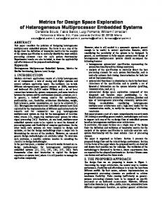
We present the SEQUITUR algorithm for lossless on-line compression of traces. The trace can be seen as a string over the alphabet of memory references. SEQUITUR represents a string σ via context free grammar whose language is the singleton set {σ}. Rules of the grammar capture the hierarchical structure of the trace; thus, the grammar is typically far more compact than the original trace. The SEQUITUR algorithm adds each symbol from the input string to the end of grammar’s start production and restructures the rules of the grammar to maintain the following invariants: Invariant 1 No pair of adjacent symbols appear more than once in the grammar Invariant 2 Every rule (except the rule defining the start symbol) is used more than once. To intuitively understand the algorithm, we briefly describe how it works on the string 123123. After reading the first four symbols, the grammar consists of the single production rule S → 1231 (where S is the start symbol). On reading the fifth symbol, it becomes S → 12312. Since the adjacent symbols 12 appear twice in this rule (violating the first invariant), SEQUITUR introduces a non-terminal to get S → A3A

A → 12

Note that here the rule defining non-terminal A is used twice. Finally, on reading the last symbol of the string 123123 the above grammar becomes S → A3A3

S −> BB B −> 123

B

1

2

3

Figure 1: SEQUITUR grammar and DAG corresponding to the trace 123123

BACKGROUND

In this section, we provide the relevant background needed for explaining our cache simulation technique. First, we describe SEQUITUR [13], the heart of the compression algorithm used by us for deriving space efficient trace representation. We then describe a data structure called Generalized Binomial Forest (GBF). It was developed by Sugumar and Abraham [20, 21] for simulating an uncompressed trace against multiple cache configurations in a single pass.

3.1

S

A → 12

This grammar needs to be restructured since the symbols A3 appear twice. SEQUITUR introduces another non-terminal to solve the problem S → BB B → A3 A → 12 However, now the rule defining non-terminal A is used only once. So, this rule is eliminated to produce the final result.

Note that the grammar accepts only the string 123123. S → BB

B → 123

The generated grammar can also be represented as a Directed Acyclic Graph (DAG) [10]. Figure 1 shows the grammar and the DAG corresponding to the input trace 123123.

3.2

Generalized Binomial Forest (GBF)

Generalized Binomial Forest (GBF) [20] is an efficient data structure to represent the contents of multiple caches by exploiting containment relationship among them. As this data structure is used for single pass cache simulation, the following operations need to be efficiently performed for an incoming address: (1) search to find out the hit/miss for all cache configurations, and (2) update to reflect the state of all the caches after the address is processed. Let CSL (N ) denote a cache configuration with 2S cache sets, the degree of associativity N and cache line size of 2L bytes. Then GBF can represent a group of cache configurations {CSL (n) | Smin ≤ S ≤ Smax ; n ≤ N }, where 2Smin is the smallest number of cache sets and 2Smax is the largest number of cache sets present among the group of cache configurations. For n = 1 (i.e., a direct mapped cache), we adopt a shorthand to write CSL (1) simply as CSL . Note that GBF representation assumes a Least Recently Used (LRU) policy. However, it can be suitably modified to accommodate certain other replacement policies such as FIFO. We first explain a simpler data structure called Binomial Forest containing one or more Binomial Trees which is used as a basis to develop GBF. A binomial forest can represent a group of direct mapped caches {CSL | Smin ≤ S ≤ Smax }. The binomial forest consists of 2Smin binomial trees, one corresponding to each set in CSLmin . A binomial tree can be defined recursively as follows. A binomial tree of degree 0 (B0 ) is a single node. A binomial tree of degree k (Bk ) is obtained from two binomial trees of degree k − 1 (Bk−1 ) by making the root of one as a child of the root of the other. The number of nodes in a binomial tree of degree k is 2k . The recursive definition of a binomial tree of degree k is illustrated in Figure 2. Binomial forest is a natural data structure to represent a group of direct mapped caches. It exploits the fact that L . In the content of CSL is included in the content of CS+1 L particular, let p1 and p2 be two cache sets in CS+1 with S least significant bits as identical and equal to p. Let the content of these cache sets be x1 and x2 (they can be empty as well). Then the content of cache set p in CSL will be either x1 or x2 depending on whichever is accessed last.

Bk

B k−1

B k−1

L C 3

000

L C 2

100

001

110

011

000

101

010

111

L C 1

001

010

110

010

011

100

101

110

111

001

100

101

011

Figure 2: Definition of Binomial Tree 000

The binomial forest for the cache configuration CSLmax consists of 2Smax binomial trees of degree 0 — one corresponding to each set; the binomial forest for CSLmax −1 consists of 2Smax −1 binomial trees of degree 1 each, and so on. L Note that the binomial tree for set s in Ci−1 is obtained by combining the binomial trees for set s and 2i−1 + s in the forest for CiL . Among these two sets (i.e., s and 2i−1 + s) we check which one was accessed last; the root of the corresponding binomial tree in CiL forms the root of binomial L tree for set s in Ci−1 . The aforementioned combination of binomial trees is followed till the binomial trees corresponding to each of the cache sets in CSLmin is obtained. Note that if Smin = 0, then the binomial forest contains only a single binomial tree (since the cache has a single set). The resulting binomial forest succinctly represents all the information needed to find the content for each of the constituent cache configurations. Figure 3 depicts the construction of a binomial tree for direct mapped cache configurations with 1 − 8 sets. For an incoming address, its index part is used to search in the appropriate binomial tree. The search exploits the structure of the binomial tree such that in a tree of degree k, at most k nodes have to be searched. Once the index matches at a node, the tags are checked for match. If the tags match, then the address is a hit corresponding to all the cache configurations represented by the subtree rooted at the matched node. This node now becomes the most recently used reference and is moved up to the root of the binomial tree with a series of transformations. We now describe the Generalized Binomial Forest (GBF), which is a forest of Generalized Binomial Trees (GBT). A Generalized Binomial Tree (GBT) can be thought of as a more general form of binomial tree where each set can contain a list of length at most n for n-way set-associative caches. The elements in the list are ordered according to Least Recently Used (LRU) replacement policy. The combination procedure is modified accordingly. A GBT can be defined recursively as follows. A GBT of degree zero (B0 (n)) is a list of length n. A GBT of degree x (Bx (n)) is constructed by putting together two GBTs of degree x−1 (Bx−1 (n)) and 0 Bx−1 (n)). The root list of the resulting GBT will contain the most recently accessed n references in either root lists of the two input GBTs. Figure 4 shows an example. Assume 0 that Bx−1 (4) and Bx−1 (4) are the GBTs corresponding to two sets s1 and s2 that map to the same set s in the next smaller cache configuration. Then the root list of the GBT Bx (4) represents the content of set s, while the remaining

111

110 L C 0

010

100

001

000

101

011

111 Order in which sets were updated 000,111,100,010,011,101,001,110

Figure 3: Construction of Binomial Forest

lines along the two branches represent the content of s1 and s2 that is not present in s. In order to represent a group of cache configurations {CSL (n) | Smin ≤ S ≤ Smax ; n ≤ N }, we will need 2Smin GBTs — one for each set in the smallest cache. The GBT is searched and updated in a manner similar to binomial tree. A detailed description of GBTs as well as their search and update procedure can be found in [20].

4.

COMPRESSION DOMAIN SIMULATION

In this section, we describe our technique for cache simulation over compressed traces. We start with simulation of a single cache configuration and extend it to simulating multiple cache configurations in a single pass of the compressed trace.

4.1 Cache simulation over compressed trace The context free grammar generated by SEQUITUR algorithm captures the repeating memory reference sequences present in the trace. The grammar opens up the opportunity to perform cache simulation for each repeating sequence only once and thereby reducing the simulation time significantly. This goal can be achieved by traversing the DAG corresponding to the grammar in a bottom-up fashion. Note that each internal (non-leaf) node R in the DAG represents a finite sequence of memory references TR that appears at least twice in the trace (Invariant 2 in Section 3.1). We simulate TR starting with an empty cache and the result is stored in R. This simulation result is used by R’s parent nodes, thereby saving repeated simulation of TR . For example, in Figure 1, the sequence 123 is repeated twice and

Bx-1(4)

B’x-1(4)

Bx(4)

1

a

1

2

b

2

3

c

a

4

d

3

T

T’

4

b

T

c d T’

/* Initialization*/ hit(R) ← hit(Y1 ); local miss(R) ← local miss(Y1 ); cache state(R) ← cache state(Y1 ); /* Process the symbols from left to right */ for i → 2 to n do /* Update hit array */ hit(R) ← hit(R) + hit(Yi ); /* Resolve local misses of Yi */ temp state ← cache state(R); foreach x ∈ local miss(Yi ) do if x ∈ temp state then hit(R) ← hit(R) + 1; else if x is a local miss in R then append x to local miss(R); insert x into temp state; end /* Update cache state */ UPDATE(cache state(R), cache state(Yi )); end Algorithm 1: Processing a grammar rule R → Y1 Y2 · · · Yn for simulating one cache configuration

Figure 4: Generalized Binomial Tree this fact is captured in the DAG by the internal node B. Once we have computed the result for B by simulating the sequence 123, it can be used to compute the cache miss at S. We now present (1) what information needs to be stored at a node R after simulation of the corresponding sequence TR is complete, and (2) how the cache miss of a node is computed from its children. Without loss of generality, we assume an N-way set-associative cache with LRU replacement policy. Direct-mapped and fully-associative caches are just instances of set-associative caches. Also, it is possible to simulate other replacement policies by modifying the information stored at a node accordingly. Let TR be the sequence of memory references represented by an internal node R. Let m be a memory reference in TR and let sm be the cache set that m maps to. If TR is simulated in isolation starting with an empty cache, the following are the possible outcomes when m is looked up. • Local miss: m results in a miss and there are less than N unique references to cache set sm in TR before m (where N is the associativity of the cache). • Global miss: m results in a miss, but it is not a local miss. • Hit: m results in a hit. If the outcome of m is a global miss or hit, it is not affected by the cache state before TR . However, if the outcome of m is a local miss, then it may hit or miss in the global trace depending on the cache state before TR . Based upon the above observation, we store the following information at a node R of the directed acyclic graph corresponding to the SEQUITUR grammar. • hit(R): Number of hits in TR . • local miss(R): Sequence of local miss references for each cache set in the order in which they appear in

TR . Note that there can be at most N local misses per cache set. • cache state(R): Cache content after simulating TR . For a leaf node m denoting a single memory address hit(m) = 0, local miss(m) and cache state(m) contain m in the corresponding cache set. Let R be an internal node (non-terminal) corresponding to the grammar rule R → Y1 Y2 · · · Yn (Y1 · · · Yn are children of node R). As any non-terminal in SEQUITUR grammar is defined using exactly one rule, it is possible to compute 1 result of R given the simulation results of the simulation its children. Algorithm 1 does the processing of the rule R → Y1 Y2 · · · Yn to compute the hits, local misses and cache state for the trace representing R. In the first step of the algorithm, the hits, local misses and cache state are initialized. We then process the terminal/nonterminal symbols on the r.h.s of the rule from left to right to update each of these three quantities. In Algorithm 1, the variable temp state is initialized to the state of the cache after processing the grammar symbols Y1 , Y2 , . . . , Yi−1 . For each of the local misses x of a child node Yi , the algorithm checks if it is a local miss, global miss, or a hit given the sequence represented by Y1 , Y2 , . . . , Yi−1 as the context; it then updates the local miss and hit accordingly. Let m1 , m2 , . . . , mni be the memory address sequence corresponding to symbol Yi and let the local misses among these addresses be mi1 , mi2 , . . . and so on. When we resolve the local miss mi2 (to find out whether it is a hit or a global miss) the variable temp state has only been updated with mi1 and not the addresses between mi1 and mi2 . In other words,to resolve the local misses, we only consider the preceding local misses of Yi and the cache state after Y1 , . . . , Yi−1 . Updating with the local misses is required because the contents of each cache set is actually maintained as a sequence depending on the replacement policy in question. To see why updating with only local misses is sufficient, note that given a cache state whether an access is a hit or a

miss is determined only by the cache contents and not the usage ordering among the contents of a cache set. Clearly, the hits in Yi do not change the cache contents; they only reorder the sequence of elements in a cache set. Furthermore, no global miss can precede a local miss by definition. Therefore, to resolve a local miss of Yi , it is sufficient to consider the preceding local misses in Yi , and the cache state after Y1 , . . . , Yi−1 (which is maintained by the variable temp state in Algorithm 1). The procedure invocation U P DAT E(cache state(R), cache state(Yi )) updates cache state of R with cache state of Yi , such that it reflects the cache state for the segment of trace Y1 Y2 · · · Yi . Later symbols Yi+1 · · · Yn will be processed against this updated cache state. Figure 5 shows an example of compression domain simulation for a direct mapped cache with two sets and a rule E → ABC. Addresses 0 and 2 map to cache set 0 and addresses 1 and 3 map to cache set 1. The memory access sequences corresponding to the symbols A, B, and C are shown in the Figure. The hit, local miss, and cache states corresponding to each symbol are also shown. For the sequence 01220 corresponding to the symbol A, 0 and 1 are local misses (stored in local miss array), the first access to 2 is a global miss, the second access to 2 is a hit, and the second access to 0 is also a global miss. The final cache state corresponding to this sequence contains 0 and 1. While processing the rule corresponding to symbol E, we first add up the number of hits for A, B, and C. In addition notice that some of the local misses may become hits in E. An example is the local miss of address 0 in B. It becomes a hit in E. The cache set 1 in the final cache set(E) contains 1 from cache state(C). However, the 0th cache set in cache state(C) is empty. It is filled up in cache set(E) by 2 from the cache state(B). As mentioned before, the source of performance improvement by processing a compressed trace comes from the fact that a rule represents a segment of trace which appears multiple times. All references except local misses only need to be processed once. The overheads involved are the time required to look up the local misses and to update the cache state for each rule. As the SEQUITUR algorithm achieves high compression ratio, indicating that typically a rule appears multiple times, the overheads are offset by the time saved in processing each rule only once.

4.2

Simulating Multiple Configurations

In this section, we present an algorithm to simulate multiple cache configurations in one pass over the compressed trace. The multiple cache configurations have fixed cache line size, variable number of cache sets and degree of associativity. Using the terminology from Section 3, we are interested in exploring the design space represented by {CSL (n) | Smin ≤ S ≤ Smax ; n ≤ N }. Smin is the smallest number of cache sets and Smax is the largest number of cache sets present among the cache configurations in the design space. Our simulator reports the hit rate for all the cache configurations in a single pass. This information can be used by the designer to choose an appropriate configuration given the constraints. Note that our simulator has to be invoked for each different cache line size. However, as observed in [5], varying

cache line size is not common as it requires significant reengineering of processor and memory data path as well as their interfaces. Similarly, we assume LRU replacement policy and write-allocate caches, which are the most common choices. A separate run of the simulator will be required for each of the different choices of replacement and write allocation policies. Our algorithm traverses the grammar in the same way as single cache configuration presented in Section 4.1. However, the information that needs to be stored at node R is modified as follows. • A two dimensional array hit(R). • local miss(R) for CSLmax (N ), the largest cache configuration. The references in local miss(R) can not be hit in smaller cache configurations. • A forest of General Binomial Trees GBF (R) described in Section 3, which is a compact representation of multiple cache configurations. The idea is to efficiently capture the hit, local miss and cache state of multiple cache configurations. First, we use a two-dimensional array hit(R) instead of a single value to maintain the number of hits corresponding to a symbol. However, hit(R)[m][n] only stores the number of references L that hits in cache configuration Cm (n) but misses in all the 0 0 0 0 L smaller caches Cm 0 (n ) where (m ≤ m, n < n) or (m < m, 0 n ≤ n). This is because, the hits in smaller caches will definitely be hits in larger caches. Thus, the total number of hits L of Cm (n) can be computed by accumulating the hit count L 0 0 of itself and those from the smaller caches Cm 0 (n ) (m ≤ m and n0 ≤ n) at the end of the simulation. The time for this post-processing of hit counts is of course negligible. We maintain the local misses corresponding to the largest cache configuration CSLmax (N ). This is justified by the fact that all the local misses of smaller cache configurations will definitely be included in the local misses of CSLmax (N ). Finally, GBF (R) succinctly captures the content of all the cache configurations after simulating the sequence corresponding to R. Figure 6 illustrates how multiple cache configurations are simulated over compressed trace by processing each rule. For a non-terminal node E in the DAG, the GBFs of its children are merged together to generate the GBF corresponding to E. The local misses are resolved to update the hit array and generate the local miss array of E. The detailed algorithm is given next. Let R be an internal node corresponding to the grammar rule R → Y1 Y2 · · · Yn (Y1 · · · Yn are children of node R). Algorithm 2 computes the simulation result of R given the simulation results of its children. Each local miss x in Yi is searched in the generalized binomial tree corresponding to the cache set of x in the smallest cache configuration. However, we use an efficient search procedure that starts searching from the middle of a GBT instead of from the root. This can be done because x will first encounter other local misses of Yi in the search path (which are the most recently used references). However, we already know the result of looking up x against that sequence from the simulation of Yi . So we can start searching from the first node in the GBT which is not from Yi . The search continues till either the address is a hit, or a leaf node is reached. The

CS(E) Hit = 3 0 1 E LM(E)

CS(A) A

01220 Hit = 1

0 1 LM(A)

2 1 Direct mapped cache with 2 sets LM = Local Misses CS = Cache State at the end of simulation

CS(B) B

0 1

CS(C) C

2 3

1

0322 Hit = 1

0 3 LM(B)

1 Hit = 0

1 LM(C)

Figure 5: Example of compression domain simulation /* Initialization*/ hit(R) ← hit(Y1 ); local miss(R) ← local miss(Y1 ); GBF (R) ← GBF (Y1 ); /* Process the symbols from left to right */ for i → 2 to n do /* Update hit array */ hit(R) ← hit(R) + hit(Yi ); /* Resolve local misses of Yi */ temp GBF ← GBF (R); foreach x ∈ local miss(Yi ) do search x in temp GBF ; if x is a hit then update hit(R); else if x is a local miss in R then append x to local miss(R); update temp GBF to insert x; end /* Update cache state */ UPDATE(GBF (R), GBF (Yi )); end Algorithm 2: Processing a grammar rule for simulating multiple cache configurations

hit and local miss array are updated accordingly and the GBT is modified to represent the new state of the cache. The U P DAT E routine merges the cache state represented by GBF (R) after processing rules Y1 . . . Yi−1 with that of GBF (Yi ) to represent the state of the cache for the sequence Y1 . . . Yi . The U P DAT E routine looks up the references present in GBF (Yi ) one by one in GBF (R). For each reference x in GBF (Yi ), the search of GBF (R) can again bypass all the references of GBF (Yi ) that appear before x. However, in this case the search is simpler as the hit and local miss array are not updated.

4.3

Implementation Issues

We discuss two major implementation issues in this section. First, the memory requirement to maintain GBTs cor-

E LM = Local Misses GBF = Generalized Binomial Forest

A

B

C

LM(E)

GBF(E)

GBF(A)

LM(A)

GBF(B)

GBF(C)

LM(B)

LM(C)

1

Figure 6: Simulating multiple cache configurations.

responding to all the grammar rules can be prohibitively expensive. We discuss a memory management scheme to alleviate this problem. This allows our simulation technique to scale up w.r.t. size of the caches and the number of cache configurations. Secondly, we discuss specific improvements made to the SEQUITUR algorithm to make the compressed trace suitable for cache simulation. We use an array based implementation of Generalized Binomial Tree [20]. It is more efficient than manipulating pointer-based data structures. For a group of cache configurations {CSL (n) | Smin ≤ S ≤ Smax ; n ≤ N }, a forest of GBTs is represented as 2Smin two dimensional arrays, each with 2Smax −Smin +1 − 1 rows and N columns. The array implementation has a factor of two redundancy. However, note that we need a GBF for each rule in the grammar generated by SEQUITUR, which may require considerable amount of memory. For example, to simulate multiple cache configurations with cache sets ranging from 1 to 256, and set associativity from 1 to 4, each rule needs roughly 8KB. Assuming that the grammar has ten thousands rules, the memory al-

1

located for GBFs is 80MB. Besides, we also need to allocate memory for hit array and local misses for each rule. Thus the total memory usage can be above 100MB. With larger range of cache configurations, there will be significant swapping. However, we observed that, in practice, for the majority of the rules, the GBTs are far from being full. On an average, only about 20% of the GBT array is used for the set of cache configurations and benchmarks we have studied. Recall that our SEQUITUR grammar representation of the trace can be represented as a directed acyclic graph (DAG). We observed via experiments that typically, the GBTs for only a few nodes near the root of the DAG are close to full. Based on these observations, we allocate a working pool of GBTs in the memory at the very beginning. A rule R is processed using the GBTs from the working pool. Once the processing is finished, the GBTs corresponding to R are converted into a more compact format and stored away. Later on, when R is required again by its parent(s), the GBTs are constructed again from the compact format. This approach cuts down the memory usage and subsequent swapping considerably. We also make several modifications to SEQUITUR algorithm to make it more suitable for cache simulation. First, the original grammar generated by SEQUITUR often contains rules with very few symbols. This can cause many problems: (a) the grammar will contain many rules and hence will require considerable amount of memory for processing, and (b) there is a lot of overhead in processing a short rule. Let us elaborate the second point. Simulation over compressed trace will be efficient only if there are lot of references that generate global misses and hits within a rule. This is because only these references need to be processed once, whereas references corresponding to the local misses need to be processed more than once. Within a short rule, there are very few global misses or hits and local misses are dominant. To solve this problem, we do some postprocessing of the grammar generated by the SEQUITUR algorithm. The short rules below some threshold are eliminated via inlining. The post-processed grammar will typically have less number of rules and the rules are longer. The grammar generated by SEQUITUR algorithm also has the obvious problem that it requires log(n) rules to represent a sequence xn as it uses hierarchical representation. Instead, we use run-length encoding to represent these sequences. For example, we represent the sequence xxxx as A → x(4) instead of B → AA; A → xx. The run-length encoding has two benefits: (a) it reduces the number of rules and therefore it is more compact and requires less memory, (b) it reduces the processing time for the sequence. The second point needs some explanation. First, note that the final cache state and the local miss sequence for xn is the same as the symbol x. The only thing that needs to be modified is the number of hits of xn as it needs to include the local misses of x that generates hit in xn . Again the number of extra hits is the same for the second to nth instances of x. Finally, for benchmarks with huge traces, we divide the trace into multiple sub-traces and generate grammar for each. This is done to avoid generating huge grammars and keep the number of rules between thousands to ten thousands. In our experiments, we generate a grammar for every 128MB of a trace.

5.

EXPERIMENTAL RESULTS

We evaluate the efficiency of our technique by comparing it against the fastest known cache simulator Cheetah. Cheetah is an accurate single pass cache simulator over uncompressed traces that implements the algorithm based on Generalized Binomial Forest. Our technique also produces accurate cache hit/miss rates. This is because we perform exact simulation (even though in a single pass) and employ a lossless compression scheme. In other words, we do not use any approximation. However, our technique achieves significant speedup compared to Cheetah as it works on compressed traces. We select programs from MiBench [7], an embedded benchmark suite, for our experiments. The description of the benchmarks chosen is given in Table 1. The benchmark programs are compiled and simulated by SimpleScalar toolset[2] with some code plugged into the simulator to collect traces. We report experimental results for data caches only. Instruction traces have more regularity than data traces, which result in higher compression ratios. Therefore, the speedups obtained by simulating over compressed traces are observed to be higher for instruction traces (compared to the speedups that we report here for data memory traces). We simulate cache configurations with 1 to 256 cache sets, degree of associativity from 1 to 4, and 16-byte cache lines. That is, a total of 24 cache configurations are simulated in a single pass. The experiments are performed on a Pentium IV 1.3GHz computer with 1 GB main memory. Both Cheetah and our simulator are compiled with the same optimization options. The performance results are presented in Table 2. Column Uncompressed gives sizes of raw traces which Cheetah uses for simulation. Column Compressed gives sizes of compressed traces. For most benchmarks, the SEQUITUR grammar along with our optimization achieves a compression ratio of more than 10. The simulation timings for Cheetah and our method are given in the columns Cheetah and Our method respectively. The Ratio column gives the speedup of simulation time that our work achieves over Cheetah. For most benchmarks, the speed-ups are significant. The last two benchmarks rijndael and typeset achieve little speed-up. This is because not much compression is achieved due to the irregular data access in these traces. Table 2 also indicates that the speedup is not proportional to the compression ratio. This is because the processing of a node in the directed acyclic graph (for the SEQUITUR grammar) has overheads in terms of resolving the local misses and combining the cache states of its children. Table 3 gives more insight into the behaviors of the two simulators. In both cases, we need to perform search and update of GBTs, which are the most time consuming operations in both the simulators. The column Search show the number of addresses that are looked up in GBTs for both the simulators. In case of Cheetah (uncompressed trace), this is exactly same as the number of memory references present in the trace. In our method (compressed trace), the number of searches is cut down significantly as the hits and global misses are only searched once. Columns under Compare show the total number of nodes in the GBT that are looked up during the search. This number is also significantly less in our method compared to Cheetah. Finally, column Local miss gives the percentage of local misses in the rules. These numbers justify one of the major sources of the speedup that

Program basicmath bitcount cjpeg djpeg dijkstra FFT ghostscript gsm(encode) gsm(decode) ispell lame patricia rijndael typeset

Description Performs simple mathematical calculations Counting the number of bits in an array of integers JPEG image compression JPEG image decompression Computing shortest paths between pairs of nodes in a graph Fast Fourier Transform on an array of data A postscript language interpreter Encoding of GSM voice communication standard Decoding of GSM voice communication standard A Spelling checker A MP3 enocder Representing trees of sparse leaf nodes with Patricia trie A block cipher selected by AES A general typesetting tool

Table 1: Description of benchmark programs.

Program basicmath bitcount cjpeg djpeg dijkstra FFT ghostscript gsm(encode) gsm(decode) ispell lame patricia rijndael typeset

Trace size (MB) Uncompressed Compressed 160 2.9 291 3.5 107 29.3 44 4.7 339 19.7 122 9.4 1209 45.7 1583 62.6 296 45.6 1191 83.9 204 13.6 847 44.3 797 480.8 85 43.2

Ratio 55.17 83.14 3.65 9.36 17.21 12.98 26.46 25.29 6.49 14.20 15.00 19.12 1.66 1.97

Cheetah 12.34 18.17 10.67 3.47 29.11 9.36 104.24 132.20 18.96 94.82 16.73 68.21 88.52 9.11

Time (sec) Our Method 2.81 1.32 5.77 1.12 13.54 2.95 26.59 17.27 8.18 39.88 4.87 18.41 84.94 8.64

Ratio 4.39 13.77 1.85 3.10 2.15 3.17 3.92 7.65 2.32 2.38 3.44 3.71 1.04 1.05

Table 2: Comparison of single pass simulation for uncompressed (Cheetah) and compressed traces (Our method).

Program basicmath bitcount cjpeg djpeg dijkstra FFT ghostscript gsm(encode) gsm(decode) ispell lame patricia rijndael typeset

Uncompressed 41.97 76.52 28.14 11.72 89.10 32.20 317.12 415.06 77.67 312.32 53.62 222.08 209.01 22.40

Search Compressed 5.15 2.20 11.50 2.12 24.75 5.57 52.42 31.66 15.54 69.03 9.20 32.73 133.62 15.42

Ratio 8.15 34.79 2.45 5.53 3.60 5.60 6.05 13.11 5.00 4.52 5.83 6.79 1.56 1.45

Compare Uncompressed Compressed 193.98 20.92 272.44 7.03 172.75 63.61 51.82 7.23 504.68 136.27 147.21 21.66 1670.40 204.45 1929.99 124.30 279.87 69.02 1487.94 335.68 284.97 44.10 1065.83 151.37 1505.82 1105.02 156.47 91.93

Ratio 9.27 38.75 2.72 7.16 3.70 6.80 8.17 15.6 4.05 4.43 6.46 7.04 1.36 1.7

Local Miss (%) 2.94 10.09 6.12 14.08 10.26 4.49 3.06 4.98 4.92 6.11 9.05 5.39 0.08 4.79

Table 3: Sources of speedup for our method (numbers of search and compare are in millions)

our work can achieve. Only less than ten percent of the addresses that are looked up in a rule are local misses for most benchmarks. Therefore, most addresses are either hits or global misses, which do not need to be processed further. Note that benchmark rijndael has the lowest percentage of local misses; however, its speedup is the lowest. This is because the compression ratio for rijndael is very low, i.e., there are very few repetitive patterns. In summary, the combination of compression ratio and the length of the rules determine the performance of our simulator.

6.

DISCUSSION

In this paper, we have discussed a time and space efficient technique for simulating a compressed trace against multiple cache configurations. The simulation proceeds by a single pass of the compressed trace representation. We have implemented our technique and we report experimental results for MiBench programs. The results indicate substantial gains in simulation timings (as compared to existing work on simulating an uncompressed trace against multiple cache configurations [20, 21]). The major application of our simulation strategy is for design space exploration of caches. It is an exact and efficient technique which can simulate huge traces of realistic programs (upto 1GB) against large number of design points (i.e., cache configurations). In a broader perspective, we note that the recent years have seen substantial work in using compressed traces for profile-driven analysis [10], deciding data layout [18], program optimization and debugging [24]. This paper demonstrates another application of compressed traces, specifically for embedded processor design.

7.

ACKNOWLEDGMENTS

This work was partially supported by a InfoComm and InfoTech Initiative (ICITI) research project R252-000-150112 at the National University of Singapore. We thank the anonymous referees for their helpful comments.

8.

REFERENCES

[1] Altera. Nios embedded processor system development. http://www.altera.com/products/ip/processors/ nios/nio-index.html. [2] Douglas C. Burger and Todd M. Austin. The SimpleScalar tool set, version 2.0. Technical Report CS-TR-1997-1342, University of Wisconsin, Madison, June 1997. [3] Trishul M. Chilimbi. “Efficient representations and abstractions for quantifying and exploiting data reference locality”. In PLDI, 2001. [4] P. Faraboschi et al. Lx: a technology platform for customizable VLIW embedded processing. In ISCA, 2000. [5] A. Ghosh and T. Givargis. “Analytical design space exploration of caches for embedded systems”. In Design Automation and Test in Europe (DATE), 2003. [6] R. E. Gonzalez. Xtensa: A configurable and extensible processor. IEEE Micro, 20(2), 2000. [7] M. Guthaus, J. Ringenberg, D. Ernst, T. Austin, T. Mudge, and R. Brown. MiBench: a free, commercially representative embedded benchmark suite. In IEEE Intl. Workshop on Workload Characterization, 2001.

[8] M. D. Hill and A. J. Smith. “Evaluating associativity in CPU caches”. IEEE Transactions on Computers, 38(12):1612–1630, December 1989. [9] S. Laha, J.H. Patel, and R.K. Iyer. Accurate low-cost methods for performance evaluation of cache memory systems. IEEE Transactions on Computers, 37(11), 1988. [10] J. R. Larus. “Whole program paths”. In PLDI, May 1999. [11] Y. Li and J. Henkel. “A framework for estimating and minimizing energy dissipation of embedded HW/SW systems”. In Design Automation Conference, 1998. [12] R. L. Mattson, J. Gecsei, D. R. Slutz, and I. L. Traiger. “Evaluation techniques for storage hierarchies”. IBM Systems Journal, 9(2):78–117, 1970. [13] C. G. Nevill-Manning and I. H. Witten. “Linear-time incremental hierarchy inference for compression”. In Data Compression Conference(DCC’97), pages 3–11, 1997. [14] M. Oskin, F.T. Chong, and M. Farrens. HLS: Combining statistical and symbolic simulation to guide microprocessor designs. In ISCA, 2000. [15] P.R. Panda, N.D. Dutt, and A. Nicolau. “Architectural exploration and optimization of local memory in embedded systems”. In International Symposium on System Synthesis (ISSS 97), 1997. [16] P.R. Panda, N.D. Dutt, and A. Nicolau. “Data cache sizing for embedded processor applications”. In Design Automation and Test in Europe (DATE), 1998. [17] T. R. Puzak. Analysis of cache replacement algorithms. PhD thesis, University of Massachusetts, Amherst, February 1985. [18] S. Rubin, R. Bodik, and T. Chilimbi. “An efficient profile-analysis framework for data layout optimizations”. In Principles of Programming Languages (POPL02), January 2002. [19] W-T. Shiue and C. Chakrabarti. Memory exploration for low power embedded systems. In Design Automation Conference, 1999. [20] R. Sugumar and S. Abraham. Set-associative cache simulation using generalized binomial trees. ACM Transactions on Computing Systems, 13(1), 1995. [21] R. A. Sugumar and S. G. Abraham. “Efficient simulation of multiple cache configurations using binomial trees”. Technical Report CSE-TR-111-91, CSE Division, University of Michigan, 1991. [22] Wen-Hann Wang and Jean-Loup Baer. “Efficient trace-driven simulation methods for cache performance analysis”. In Proc. 1990 ACM SIGMETRICS Conf. on Measurement and Modeling of Computer Systems, pages 27–36, May 1990. [23] Z. Wu and W. Wolf. “Iterative cache simulation of embedded CPUs with trace stripping”. In International Workshop on Hardware/Software Codesign, 1999. [24] Y. Zhang and R. Gupta. Timestamped whole program path representation and its applications. In PLDI, 2001.