performing design verification of switching power convert- ers. The first method can ... verification for all runs of the circuits and all possible component parameter ...
Design Verification Methods for Switching Power Converters Taylor T. Johnson, Zhihao Hong, and Akash Kapoor Dept. of Electrical and Computer Engineering University of Illinois at Urbana-Champaign Urbana, IL 61801 Email: {johnso99, hong64, akapoor5}@illinois.edu Abstract—In this paper, we present two methods for performing design verification of switching power converters. The first method can be used to compute the set of reachable states from an initial set of states with nondeterministic parameters. We demonstrate the method on a buck converter in an open-loop configuration. The method is automatic and uses the hybrid systems reachability analysis tool SpaceEx. The second method uses model checking to verify circuits that can naturally be modeled as timed automata. We demonstrate the method on an openloop multilevel converter used to convert several DC inputs to one AC output. The method is also automatic and uses the timed automata model checker Uppaal. Finally, we mention that in contrast to simulation or testing based approaches—for instance, the standard Monte Carlo analysis used when analyzing component variation in circuit designs—the methods presented in this paper perform the verification for all runs of the circuits and all possible component parameter variations. Index Terms—hybrid systems, verification, buckconverter, multilevel converter
I. I NTRODUCTION A traditional method used to validate that a circuit design is behaving according to its requirements is to first run a few simulations, then perhaps perform a Monte Carlo analysis varying the circuit elements within their tolerances. However, all such methods are incomplete, in the sense that they cannot try all possible combinations of parameter variations or all initial conditions. That is, each iteration of such a method corresponds to a single execution of the system, and since there are uncountably infinitely many such executions, any method would run forever. More recent techniques apply reachability and verification methods from hybrid systems research to circuits, such as [1], [2], [3], which may allow one to check all possible parameter variations and use sets of initial conditions. These reachability techniques rely on computing an overapproximation of the reach set of a system, which is the set of all trajectories of the system from some set of initial conditions (sometimes allowing for variation
in the parameters of the system). For many classes of systems, computation of the reach set for unbounded time is either undecidable or computational impractical, so frequently a time-bounded reach set is used, which is the reach set up to some finite time. More concretely, the reach set from time t0 to t f is t Rt0f
n
= {x ∈ R : x =
Z t t0
f (x(τ))dτ, x(t0 ) ∈ x0 ,t ∈ [t0 ,t f ]},
for a system with dynamics x˙ = f (x) and an initial set of states x0 ⊆ Rn . Most reachability methods compute an overapproxt imation of the set Rt0f . Since these methods compute an overapproximation of the reach set, one can then guarantee that some bad (or unsafe) property does not occur (in bounded time) by ensuring the intersection of the reach set and the bad set of states is empty. If this intersection is empty, then the system is safe, but if the intersection is nonempty, one generally may not conclude that the system is unsafe. This is due to the nature of overapproximation—additional trajectories are included in the reach set that do not actually exist in executions of the actual system, i.e., the trajectories intersecting the bad set of states may be spurious and arise from the overapproximation. Concretely, in the DC-to-DC converter investigated in this paper for instance, the bad set of states would be those where the output voltage strays too far from the desired value due to voltage ripple. More concretely, if a desired output voltage is 5V, then the bad set of states could be those outside the interval [4.9, 5.1]V, or whatever the particular specification requires. In this paper, we consider application of two verification methods to ensure circuit designs satisfy their specifications. The first method is a reachability analysis method that can be used to verify switched-mode power supplies like buck-converters, boost-converters, Cuk converters, push-pull converters, and other topologies. We present it as a case study on verifying that
the output voltage of a buck-converter are within a tolerance band due to voltage ripple. Specifically, we answer two questions for the buck converter. We first present a method to answer the question of whether a particular converter design and an open-loop control (in terms of a control period and duty cycle) will satisfy a specified output voltage range. For instance, does a given buck-converter design with a 12V input always maintain an output voltage between 4V and 6V? We do not report it here for space, but a similar method answers the same question of the buck-converter with a given closed-loop control strategy. We illustrate this method using the hybrid systems reachability tool SpaceEx [4]. The second method relies on using model checking for timed automata [5] to verify properties of circuits that can be modeled as timed automata. For reference, a timed automaton is a finite-state machine with additional clock variables that evolve monotonically with time, where potentially the clock rates vary in different states of the automaton. Concretely, timed automata allow dynamics of the form x˙ = a (upon integrating with respect to time, one has x = at, which gives the reason as to why they are called clocks and timed automata). Specifically, we show that multilevel converters used to convert multiple DC inputs to a single AC output can naturally be modeled as timed automata. The contribution of this method is primarily the realization that some analog circuits can be naturally modeled as timed automata. We illustrate the method by verifying several properties of a particular multilevel converter using the timed automata model checker Uppaal [6]. Related Work: There are a variety of computational methods and tools for computing reach sets of different classes of systems, several of which have been applied to circuits [1], [2], [3], [7]. Researchers have been developing computational tools for computing reach sets and analyzing hybrid systems for some time [8], [9], [10], [11], [12], [13], [14], [15], [4], [16]. Many of these methods work by computing an overaproximation of the reach set by computing an overapproximation of the state transition function corresponding to the solution of the dynamical system (recall for the case of a linear system that the state transition function is the matrix exponential, so x(t) = eAt x0 ). For instance, several of these methods are inspired by the following idea. A bounded subset of the state space of the system is discretized into compact (frequently convex) regions. This discretization can occur either before computing the reach set, or on-the-fly during the computation (which may allow methods to discretize ”‘interesting states”’ more finely). Over each
S
L iL
VS
C
+ Vc -
R
+ Vout -
Fig. 1. Buck-converter circuit—a DC input Vs is decreased to a lower L DC output Vout .
+ + iL R Vout C Vc V S of these compact regions, the dynamics of the system are overapproximated. Since the regions are compact and
the dynamics are usually continuous, the dynamics will take a minimum and maximum over the compact set. The resulting system is aLhybrid system with dynamics defined in each compact region, and for this reason, the method is known as hybridization +[15]. If the+ original iL system is hybrid, this idea canCbe used eachVmode. Vc in R out The Ellipsoidal Toolbox [14] was used in - [3], and allows for calculation of reach sets of piecewise affine systems. One major issue in computing reach sets of systems is that the methods may scale very poorly in the number of dimensions (variables) of the system. The other obstacle to a useful reachability method is how many spurious states are reached—i.e., the overapproximation from the actual reach set should be as small as possible. For instance, the optimal control inspired methods used in the Ellipsoidal Toolbox and other methods like [17] become impractical beyond tens of variables, at best. The tool we use, SpaceEx, is the successor of the successor of the tool PHAVer [12]. One reason we were interested using SpaceEx is for future work—the support function algorithm [18] used for reach set computation in SpaceEx scales quite efficiently in the number of variables, and examples with tens and hundreds of variables are feasible, and those with thousands of variables will be feasible soon. Another method that scales quite well in the number of variables is a method using zonotypes [16], [7], which has also reached hundreds to thousands of dimensions. II. R EACHABILITY A NALYSIS FOR DC- TO -DC S WITCHMODE P OWER S UPPLIES We will briefly review a switched-system model of a buck-converter, but the interested reader is referred to an in-depth derivation of the model in [19]. A buckconverter is a DC-to-DC switchmode step-down converter. The converter takes an input voltage of say 5V and ”bucks” or drops the voltage to some lower DC voltage, say 2.5V. The circuit can be seen in Figure 1. The basic operation is that the voltage source is connected and disconnected from the load by toggling the
switch S at some switching frequency Ts and duty cycle. We will refer to the duty cycle with switch S open as 1 ≥ ∆o ≥ 0 which is the percentage of time spent with S open. Likewise, the time spent with switch S closed is referred to as ∆c = 1−∆o . In an open-loop configuration, each of Ts , ∆c , and ∆o are fixed, while in closed-loop, they may vary based on different control strategies. The position of the switch gives rise to different modes, of which there are a finite number in some index set M. In open-loop, this circuit can be modeled as a switched affine (linear with fixed input) system [20] of the following form, x˙σ(t) = Aσ(t) x + Bσ(t) , where for each i ∈ M, Ai ∈ Rn×n , Bi ∈ Rn , and σ(t) : R → M is a function mapping time to a mode. For the buckconverter, the two state variables are the current through the inductor iL and the voltage across the capacitor Vc , so we have iL . x= Vc In continuous conduction (see, e.g., [19]), there are two modes based on whether the switch is open or closed, so M = {o, c}, and each mode is described by the following system matrix, 0 − L1 . (1) Ao = Ac = 1 1 − C RC However, the affine input term differs based on the mode selection. If S is closed, then the voltage source is connected, so Bc = [ L1 ; 0]Vs , while if it is open, Bo = [0; 0]Vs . We chose not to model parasitics in favor of modeling nondeterministic parametric uncertainty in the components as described below in Subsection II-A, but one can make the extension by appropriately modifying Equation 1. With such a system definition, one may analyze stability of this system using a variety of techniques. Aside from traditional tests like Bode analysis, there are other now classic techniques like averaging analysis [21], or one can use more recent switched-system techniques [20]. Since the system is linear, such techniques may account for small perturbations in the model, for instance, due to component variation of the circuit elements. However, such techniques as just described may be unable to account for variation in the switching time itself. For these reasons, and our interest in using a computational approach, we chose to analyze stability of this system using a recent hybrid systems reachability tool called SpaceEx [4].
A. Parameter Variation Due to manufacturing processes and environmental factors (e.g., parameter variation due to temperature changes), any actual circuit implementation of the buck converter will not match the model from Equation 1. We now describe a method to capture such behaviors when performing a reachability computation. For our example, suppose we are given some tolerances for each component as shown in Table I. Due to component variation, one can no longer specify the system as a single matrix, but as a family of matrices. To overapproximate the behavior of such a system, one may use interval arithmetic and interval matrices [22], for which there exist necessary and sufficient conditions for stability [23], [24]. There are also more computational practical sufficient conditions [25]. There are some computational tools using interval arithmetic to compute reach sets [10], [16], [26]. SpaceEx does not support such interval matrices, so we describe a simple technique used to overapproximate the reach set. More precisely, an n × n interval matrix is defined as a set of real matrices:
A = {A = [ai j ] : ai j ∈ [bi j , ci j ], i, j = 1, . . . , n}, that is, each entry ai j in A varies between bi j ≤ ai j ≤ ci j . Matrices of dimension n × m for n 6= m can be defined similarly. The interval dynamic system described by x˙ = Ai x for any Ai ∈ A was shown to be asymptotically stable in [23] if and only if the matrices Ai created from all possible combinations of interval endpoints bi j and ci j are stable. Similarly, to overapproximate the reach set, it is sufficient to consider every combination of interval extrema in A . There may be an exponential number of such combinations, so the methods to overapproximate the interval matrix reach set in [26] may be better suited, but this tool was not available to us at the time of writing. For some systems, it is sufficient to compute a minimal and maximal matrix A and A respectively. These matrices satisfy the orders A ≤ A ≤ A, where ≤ means ai j ≤ ai j ≤ ai j for i, j = 1, 2, . . . , n and ai j ∈ A, ai j ∈ A , and ai j ∈ A. Using this, we can overapproximate the reach sets of A by computing reachability using A and A. Thus, for computing the reach set, we can look only at the ”worst behaved” matrices, where worst behaved essentially means the matrices with the smallest stability margins, as also used in the more computationally efficient sufficient condition for stability from [25]. Concretely, suppose we allow the component variations for R, C, and L to take each take nondeterministically from a range like the ±5% variations indicated in Table I. We can also model nondeterministic uncer-
Symbol
6
Range
Input Voltage
Vs
[11.95, 12.05] V
Load Resistance
R
[0.95, 1.05]Ω
Capacitor
C
[23.75, 26.25] uF
Inductor
L
[47.5, 52.5] uH
Control Period
Ts
[24.5, 25.5] us
Switch-open duty cycle
∆o
[9.75, 10.25] us
Switch-closed duty cycle
∆c
[14.75, 15.25] us
5
Voltage (V)
Component / Parameter Name
4 3 2
TABLE I B UCK - CONVERTER PARAMETER VALUES AND VARIATIONS .
1
tainties in the switching times simply by allowing a mode switch to occur in a range of times instead of at a the particular time designated by the control period and mode duty-cycle. We then arrive at an interval system matrix for each mode of the buck-converter as [0, 0] [−21053, −19048] , Ao = Ac = [38095, 42105] [−44321, −36281]
0 0
0.5
1
1.5 Time (s)
2
2.5
3 -4 x 10
Fig. 2. Startup verification of buck-converter output voltage using parameters from Table I. The upper red set shows the reachable states due to A, and the lower blue set shows the reachable states due to A. The initial set of states were iL ∈ [0, 0.1]A and Vc ∈ [0, 0.1]V.
7
and the input matrices as
Bo =
[0, 0] [0, 0]
and Bc =
[19048, 21053] [0, 0]
.
To compute these interval matrices, we relied on the following interval extensions of multiplication and division. For two intervals [a, b] and [c, d], we have [a, b] ∗ [c, d] = [min(ac, ad, bc, bd), max(ac, ad, bc, bd)]. Similarly, the quotient of two intervals (supposing the divisor interval [c, d] does not contain zero) is defined as [a, b]/[c, d] = [a, b] ∗ (1/[c, d]) for 1/[c, d] = [ d1 , 1c ].1 Figure 2 displays the reachable states from a startup condition, and proves that the system with the chosen parameters always has an output voltage within the range in the graph. We omit the reach set computation figure for steady-state due to space constraints, but it also satisfies a voltage ripple constraint. In Figure 3, we show the current-versus-voltage output from the hybrid systems reachability tool SpaceEx [4], which supports systems with affine dynamics (i.e., of the form x˙ = Ax+B where B is a constant vector or more generally, takes values from a convex set of appropriate dimension). 1 We
can also symbolically define this matrix, letting R be the upper value of this range for R, R be the lower value, so R ≤ R, and analogously for the other components, but do not do so because writing 1 the entry − RC is tedious with the numerous min and max operators.
Fig. 3. Current-versus-voltage plot of the reachable states from startup for the buck-converter. Units are in amps and volts.
III. M ODEL C HECKING FOR M ULTILEVEL C ONVERTERS In this section, we present a multilevel converter model and model checking procedure used to verify properties of it. A multilevel converter takes several DC voltage sources and creates an AC output as shown
vout[id] == 0 x[id] = 0, vout[id] = 0
S1
S2
x[id] >= c_level2[id] vout[id] = 0, sum_voltage()
x[id] = c_level1[id] vout[id] = vin[id], sum_voltage()
x[id]