Figure 1.Centrifugal Compressor (1). Figure 2.CentrifugalCompressor stage (1). (Used by Sir Frank Whittle) (With Kind Permission of Rolls-Royce plc) ...
DESIGNING AND TESTING OF TURBO EXPANDER H1043 INDIVIDUAL PROJECT
University of Sussex School of Engineering and Informatics Department: Engineering and Design
BEng Mechanical Engineering
Supervisor: Dr. Vasudevan Kanjirakkad Word count 8311
Candidate: 122511
Summary
This project is about making and testing of an engineering application. A knowledge of turbo-machinery and thermodynamics have involved to achieve requirements. The project is based on designing and testing of a small turbo-expander for performance. The turboexpander is essentially consist of a centrifugal compressor and a radial inflow turbine connected on a single rotating shaft. A mass flow rate of 0.048 kg/s is sucked into the compressor and transfers directly to the radial turbine, the flow path is driven by a vacuum cleaner, which is connected to the turbine exhaust. The ratio of the flow power at compressor exit to the maximum suction power from the vacuum cleaner is 56% with an overall efficiency of 35.9%. The maximum suction power from the vacuum cleaner is directly proportional to the rotational speed. This process produces energy, however, the similar flow path can be found in some other applications such as air conditioning systems in airplanes and gas liquefaction plants but with different objective, provide cold air. The project focuses on the studying of blading to match a certain boundary conditions and developing the performance of the turbo-expander components.
H1043 INDIVIDUAL PROJECT
1
CANDIDATE: 122511
Table of Contents STATEMENT OF ORIGINALITY ...........................................................................................................................3 ACKNOWLEDGMENT ........................................................................................................................................4 NOMENCLATURE .............................................................................................................................................5 CHAPTER 1: INTRODUCTION ............................................................................................................................6 CHAPTER 2: LITERATURE REVIEW.....................................................................................................................7 2.1 BACKGROUND PRINCIPLES ......................................................................................................................... 7 2.2 CENTRIFUGAL COMPRESSOR PERFORMANCE: ........................................................................................ 10 2.3 RADIAL INFLOW TURBINE PERFORMANCE:............................................................................................. 16 2.4 OPTIMUM DESIGN ..................................................................................................................................... 18 CHAPTER 3: METHODOLOGY..........................................................................................................................19 3.1 DESIGN GEOMETRY .................................................................................................................................. 20 3.2 PRELIMINARY TESTS................................................................................................................................. 21 3.2.1 Flow Rate Test ................................................................................................................................... 21 3.2.2 Frictional and Mechanical Losses: .................................................................................................. 23 3.3 BLADES PROFILING ................................................................................................................................... 26 3.4 EXPERIMENTAL SETUP.............................................................................................................................. 30 CHAPTER 4: RESULTS AND DISCUSSION .........................................................................................................31 CHAPTER 5: CONCLUSION ..............................................................................................................................35 5.1 RECOMMENDATIONS & FUTURE WORK ................................................................................................... 35 REFERENCES...................................................................................................................................................36 LIST OF FIGURES.............................................................................................................................................37 LIST OF EQUATIONS .......................................................................................................................................38 LIST OF TABLES ..............................................................................................................................................39 APPENDIX A .................................................................................................................................................... II APPENDIX B ................................................................................................................................................... III APPENDIX C ................................................................................................................................................... IV
H1043 INDIVIDUAL PROJECT
2
CANDIDATE: 122511
Statement of Originality
I declare this dissertation has been written by me for my final year individual project. It does not contain any materials that belong to other people. References have been included where applicable.
H1043 INDIVIDUAL PROJECT
3
CANDIDATE: 122511
Acknowledgment
First and foremost I would like to thank my supervisor Dr. Vasudevan Kanjirakkad for his great support in this project and his supervision. Secondly, I would like to express my thanks to the technician Simon Davies, Kevin Brady and the chief technician Peter Henderson for their kind assistance and design recommendations. I also would like to thank Dr. Romeo Glovnea for his recommendations. Last but not least, I would like to thank my family and all my friends for their support and encouragement.
H1043 INDIVIDUAL PROJECT
4
CANDIDATE: 122511
Nomenclature Symbol V β α ṁ ω N h Cf d I P r T W w ρ μ Ƞ σ Z
Quantity Absolute Velocity Blade Angle Flow Angle Mass flow rate Rotational Speed – Rotational Speed Enthalpy, Blade Height Skin Friction Coefficient Diameter Moment of Inertia of rotor Pressure Radius Torque Shaft Power Specific work Density Dynamic Viscosity Efficiency Slip Factor Number of blades
Subscripts is ov mech D r W ⍬
Isentropic Overall Mechanical Diffuser Radial Relative Swirl
o
Total or Stagnation
1
Compressor Impeller inlet
2
Compressor Impeller exit
3
Diffuser inlet
4
Diffuser exit
5
Nozzle inlet
6
Nozzle exit
7
Turbine rotor inlet
8
Turbine rotor exit
H1043 INDIVIDUAL PROJECT
5
Units m/s degree degree Kg/s rad/sec RPM J/Kg , mm mm Kg.m2 Pascal mm N.m Watt Joule Kg/m3 m2/s -
CANDIDATE: 122511
Chapter 1: Introduction The objective of the project is to design and test a small turbo-expander that will be manufactured from simple materials. The purpose of the project is to achieve the maximum possible performance at a maximum rotational speed. The project will be focusing on blades profiling of a centrifugal compressor and a radial inflow turbine to achieve requirement. In order to do this, it is vital to introduce the components of turbo-expander such as the nozzle, rotor disc, stator disc and axial shaft. The turbo-expander is driven by sucking air through the compressor intake by a vacuum pressure system that is attached at the turbine exhaust (1). The aim of the compressor is to increase the air pressure and temperature that is taken from the atmosphere and delivers it to the turbine through transfer ports. The turbine will be used to expand the compressed air and, therefore, some of its kinetic energy will be extracted to drive the compressor and the rest can be used for other applications (2). When the rotational speed is set to idle mode, the suction power from the vacuum pressure system will be dissipated by frictional losses such as mechanical friction in the bearings and fluid friction in the blades (3). This can be reduced by applying the knowledge of bearings selection. The main objective is to obtain the highest possible ratio of the flow power at compressor exit to the maximum suction power from the vacuum pressure system. This includes designing the turbo-expander from dimensions to materials selection to meet boundary conditions such as the rate of mass flow and pressure rise of the vacuum pressure system and improving its efficiency.
H1043 INDIVIDUAL PROJECT
6
CANDIDATE: 122511
Chapter 2: Literature Review 2.1 Background Principles Turbo-expander Fundamental The Term ‘Turbo-expander’ defines a single unit that consists of two primary components, compressor and expander connected on a single shaft (2). The compressor is the driven unit and the expander (turbine) is the power unit (2). Large Turbo-expanders are commonly used for gas liquefaction and power generation (4). The efficiency of the turbo-machine depends on its design, specifications and the user boundary conditions, for example, for high mass flow rate the benefit will be in the axial flow compressors while the centrifugal compressors used for a low mass flow rate, and likewise for the turbine (1). The centrifugal effects can increase the specific work input to the fluid for a given dimensions and blades profile. The centrifugal compressor stage consists of two primary components a rotating disc (impeller) and a stationary disc (diffuser). Impellers are used to increase the energy of the working fluid, the momentum of the fluid will be increased due to the centrifugal effect, whirling it radially (5).The velocity of the fluid and its static pressure rise at this stage. Therefore, the kinetic energy of the fluid will be transferred to pressure energy by the diffuser (5). The fluid will be directed to the expander so that its temperature and pressure will decrease due to expansion. Therefore, the kinetic energy of the fluid will be extracted to mechanical energy to drive the shaft. Accordingly, the laws of thermodynamics and aerodynamics are involved in designing and running turbo-expanders.
Centrifugal Compressor This section of will be focusing on the centrifugal compressor and its stages. The essential stages of the centrifugal compressor are: The eye of the impeller: This is the inlet of the impeller just after the intake nozzle. The function of the eye is to distribute the flow that sucked in through the system. The eye has an inducer or rotating guide vanes, usually finishes when the flow turns from the axial direction to radial flow (1). Some designers increase the inducer area to reduce the flow diffusion (1). The rotor disc (impeller): This component is the heart of the centrifugal compressor as its increase the velocity of the working fluid and rises its static temperature and pressure. Also, the energy level of the fluid increases due to the increase of momentum in the fluid at the impeller (1). The impeller has a series of curved vanes, shroud and hub, to guide the flow path. The shroud is the curved surface that forms the outer boundary of the flow and the hub is the inner curved surface (1). This means blades designing is an essential part for achieving high compressor efficiency. H1043 INDIVIDUAL PROJECT
7
CANDIDATE: 122511
The vaneless space: Generally, centrifugal compressors are integrated with either vaned or vaneless diffusers to convert the kinetic energy at the outlet of the impeller into static pressure. The gap between the outlet of the impeller and the inlet of the diffuser called vaneless space (1). Pressure rises in this space, hence, the larger the space the more pressure rise will occur which might affect badly on the efficiency of the compressor (3). The stator disc (diffuser): The diffuser contains a set of stationary blades that surround the impeller. They are designed in a manner that the outlet flow at the impeller will encounter an increase in flow area as it passes through them (5). As a result, this will cause a reduction in the flow velocity. The purpose of the diffuser is to control the characteristics of the fluid by converting the kinetic energy of the fluid into pressure energy, by diffusing the flow leaving the impeller, resulting in an increase in the pressure energy (5). This conversion occurs due to Bernoulli’s principle. 𝑃1 + 1⁄2 𝜌 𝑉12 + 𝜌 𝑔 ℎ1 = 𝑃2 + 1⁄2 𝜌 𝑉22 + 𝜌 𝑔 ℎ2 (1) Losses in stagnation pressure will occur if the diffusion rate is too high due to flow mixing whereas in low diffusion rate the fluid will be exposed to a long wall resulting in fluid friction losses. In general, the optimum rate of diffusion is 7o or 8o (1).
Figure 1.Centrifugal Compressor (1).
Figure 2.CentrifugalCompressor stage (1).
(Used by Sir Frank Whittle) (With Kind Permission of Rolls-Royce plc)
H1043 INDIVIDUAL PROJECT
8
CANDIDATE: 122511
Radial Inflow Turbine The radial flow turbine has similar components to the centrifugal compressor listed in the sub-section 2.2. However, the flow path entering the turbine encounters different order of stages than the compressor (4). I.e. the flow path enters the turbine through the stationary vanes, resulting the flow to pass through the vaneless space and enters the turbine rotor. The rotor has an inducer similar to the compressor. The purpose here is to receive an axial flow for a certain distance at the inducer and converts it to radial flow at the end of it as the shrouds are deflected at a set angle (5), resulting in expanding the fluid. The turbine is the power unit as it expands the high pressure energy delivered from the compressor (2). The expansion process occurs due to the shape of the blades, resulting in extracting the kinetic energy from the fluid and converting it into mechanical energy to the shaft (2). During the expansion process, the temperature of the fluid will cool down, the pressure will decrease and the flow will accelerate. This means the boundary layers are more stable and the blades can receive higher loading without boundary layer separation (1). The turbine has an exhaust (outlet nozzle) for impulse or reaction purposes.
Figure 3. Radial inflow turbine
H1043 INDIVIDUAL PROJECT
9
CANDIDATE: 122511
2.2 Centrifugal Compressor Performance: There are different methods to change the velocity of a working fluid by either changing the area of the flow (Bernoulli’s) or stream curvature (blades). The flow in a centrifugal compressor has three-dimensional motion analysis. These analysis are taken at inlet and outlet cross-section area of the impeller and the same process can be used through the machine (1). This section will illustrates velocity components and compressor performance.
Inlet Casing The working fluid enters the machine with velocity Vo to V1 and with a static pressure drop from Po to P1. In ideal conditions, the stagnation enthalpy is constant across the inlet (3). 1 1 ℎ𝑜 + 𝑉𝑜2 = ℎ1 + 𝑉12 ( 2) 2 2
The Impeller There are different types of impellers such as one sided, two sided, shrouded, unshrouded, radial, backward swept and forward swept vanes. Each type has different characteristics such the arrangement of the blades, figure4 shows some samples of impeller types.
Figure 4.samples of impeller types Flow enters the impeller with absolute velocity V, and has components of velocity, Vr, Va and V⍬, radial, axial and tangential respectively as shown in Figure 4. 𝑉 2 = 𝑉𝑟2 + 𝑉𝑎2 + 𝑉⍬2 (3) The angle made between the radial velocity and relative velocity is the exit blade angle β. If we assumed that the impeller has no guide vanes and the flow enters the impeller axially, at Va1, the velocity components Vr1 and V1 in this case will be equal to Va1. Thus, there will be no swirl component and the angular momentum of the flow is zero (6). However, the flow leaves the impeller with swirl velocity due to the centrifugal action, Vθ2 = U2 +V2 sinβ2 and Vr2 = V2 cosβ2. In ideal conditions the tangential component at outlet is equal to the impeller tip speed U2. Figure 5 shows the velocity triangle at inlet and outlet of the impeller.
H1043 INDIVIDUAL PROJECT
10
CANDIDATE: 122511
The static enthalpy change in centrifugal compressor is larger than the axial compressor, this can be explained by the following equation: 1 1 1 2 2 ) ℎ2 − ℎ1 = (𝑉22 − 𝑉12 ) + (𝑈22 − 𝑈12 ) + (𝑉𝑊1 − 𝑉𝑊2 (4) 2 2 2 1
The first term in the right hand side of equation (4),2 (V22 − V12 ), represents the actual increase in kinetic energy and the second term,
1 2
(U22 − U12 ) is the contribution from the 1
2 centrifugal effect caused by the change in radius. The third term in the equation, 2 (VW1 − 2 ), VW2 is the contribution from the diffusion of the relative velocity. Thus, in order to increase the pressure in the compressor, the work transfer across the compressor must be large. However, a high pressure ratio may lead to some aerodynamics issues such surge and stall. Compressor efficiency and blade speed effect strongly on the pressure ratio (1). 𝛾 𝑃𝑜3 ( ) = [1 + (𝛾 − 1)Ƞ𝑐 𝜎(1 − 𝜙2 𝑡𝑎𝑛𝛽2′ )𝑀𝑢2 ] 𝛾−1 (5) 𝑃𝑜1
Where, 𝜙 = 𝑉𝑟 /𝑈 and Mu = U2/ao1 is the blade Mach number.
Because the velocity changes from the inlet to the outlet, the temperature and pressure of the fluid will therefore change. In high pressure ratio compressors it might be beneficial to introduce pre-rotation to the working fluid entering the impeller to reduce its relative velocity. Pre-whirl can be achieved at the inlet by fixing guide vanes to the casing, flow enters with an angle α1, and this changes the velocity triangle at the inlet. Thus, angular deviation of the absolute velocity can be realised at the leading edge of the impeller, Vθ1 . These guide vanes act to change the pressure of the fluid at the first-stage before entering the impeller. Hence, the air density decreases as the pressure drop increases. As a result, the compressor mass flow production will decrease. Another advantage of the pre-whirl is to reduce the curvature of the impeller vanes. Therefore, the inlet guide vanes need to be designed carefully to minimise pressure losses and avoid some aerodynamics issues that will be discussed in the later stages.
𝑃 = 𝑇𝜔 = ṁ[𝑈2 𝑉⍬2 − 𝑈1 𝑉⍬1 ]
(6)
From Euler’s Equation (6), Where U = ωr, the power of the compressor is related to the tangential velocity at inlet. If the tangential velocity increases across a blade row, then the angular momentum increases and it said the work is done on the fluid (7). This can be applied for both rotating and stationary blades.
H1043 INDIVIDUAL PROJECT
11
CANDIDATE: 122511
The specific work done on the fluid will therefore be: 𝛥𝑊 = 𝑈2 𝑉𝜃2 − 𝑈1 𝑉𝜃1 (7) Form the equation above, the work done on the fluid increases with the increase of the blade speed U2 and Vθ2 (8). The second term of the equation can be neglected if the flow enters the compressor without tangential component, α1 =0, else, the work done will decreases. However, the flow will have swirl component at the outlet of the impeller, positive swirl decreases the work and negative swirl increases the work (8).
Figure 5. Velocity triangle for radial compressor (9).
Slip Factor In centrifugal compressors the relative flow at the exit of the impeller will does not receive perfect guidance from the blades therefore it will deviates. The deviation in the exit angle is called a slip. Hence, the slip factor can be introduced as ′ 𝑉𝜃2 − 𝑉𝜃2 𝜎 =1− (8) 𝑈2 ′ Vθ2 is the actual swirl velocity and Vθ2 is the ideal swirl velocity with no slip. The typical range of slip factor suggested by (Seppo A. Korpela) is 0.83< σ 0.75, to minimise the flow
separation in the impeller (11). The flow angle, α2, at the impeller exit effects on the stability of the radial vanless diffuser, therefore, as a general rule, α2 > 70o. Thus, α2 is recommended to be in the range of 60o to 65o at design point when the rotor diameter ratio is greater than 0.55 (12). The rotor diameter can be found by this relation, 𝑑 =
𝑈∗60 𝜋∗𝑁
. Blade width can be
obtained by applying Continuity equation at the outlet (13). The number of blades can be obtained by equating the slip factor ratio with Stanitz correlation, a typical blade number is between 10 and 12 (14). Designing the diffuser need more care than the impeller as the flow experienced some aerodynamics issues as mentioned in the earlier sections. The vanless space must be considered in the calculation in order to get the correct flow angles and vanes shape (1).
H1043 INDIVIDUAL PROJECT
18
CANDIDATE: 122511
Chapter 3: Methodology This chapter will focus on the design method of the centrifugal compressor and the radial turbine. Precisely, we will be meeting blades design. For design purpose, it is necessary to assume the efficiencies of the compressor and the turbine (3). Therefore, the pressure rise across the compressor and the pressure drop across the turbine can be determined by using the conventional definition of isentropic efficiency of the compressor and the turbine (3): 𝑚̇ ∆𝑃𝑐 ∆𝑃𝑡 = 𝑚̇𝜂𝑚𝑒𝑐ℎ 𝜂𝑡 (18) 𝜂𝑐 𝜌 𝜌 Where, ∆𝑃𝑐 = 𝑃𝑐𝑜𝑚𝑝 − 𝑃𝑎𝑡𝑚 and ∆𝑃𝑡 = 𝑃𝑐𝑜𝑚𝑝 − 𝑃𝑣𝑎𝑐 By rearranging equation (18), ∆𝑃𝑐 = 𝜂𝑚𝑒𝑐ℎ 𝜂𝑡 𝜂𝑐 ∆𝑃𝑡 = 𝜂𝑜𝑣 ∆𝑃𝑡 (19) Where 𝜂𝑜𝑣 is the overall efficiency which is defined as: 𝜂𝑜𝑣 = 𝜂𝑚𝑒𝑐ℎ 𝜂𝑡 𝜂𝑐 = Therefore, the objective is to maximise the function: 𝑚̇ ∆𝑃𝑣𝑎𝑐 (𝜂𝑜𝑣 /(1 − 𝜂𝑜𝑣 ) (𝑚̇ ∆𝑃𝑣𝑎𝑐 )𝑚𝑎𝑥
H1043 INDIVIDUAL PROJECT
19
∆𝑃𝑐 ∆𝑃𝑡
(20)
CANDIDATE: 122511
3.1 Design Geometry This section will illustrate the dimensions of the prototype model for this project. Figure12 shows the cross section view of the turbo-expander. The body is 440 mm2 and 186 mm deep. The shaft is 186 mm long and has a diameter of 25 mm. Sealed bearings are attached at both ends on the shaft. A Sleeve is screwed on the foam body so that bearings are securely locked from the inside and from the outside by a washer. There are two discs have been used in this design, a 200 mm outer diameter rotor and a 310 mm outer diameter stator with a 4 mm diameter vaneless space in between. The stator disc is screwed to the foam body for the sake of blades modification. Nuts will be used for tightening the washer and the rotor disc. Intake nozzle is attached on the lefthand side in figure 12 and a turbine outlet is on the other side. Figure 12.cross section view Figure 13 shows the transfer ports, 18x 30 mm. Also, it illustrates 8 holes with a 9 mm diameter for attaching a cover plate. The cover plate is 10 mm thick and it is used to maintain the flow.
Figure 13.Front view of the model
H1043 INDIVIDUAL PROJECT
Figure 14.Turbo-expander
20
CANDIDATE: 122511
3.2 Preliminary Tests This section will discuss the primary tests that carried out in order to determine the mass flow rate for a maximum suction power from the vacuum cleaner available. Also, it is necessary to estimate a value for the mechanical efficiency Ƞmech.
3.2.1 Flow Rate Test The performance of the vacuum cleaner is tested by using it to suck air through a smooth pipe to measure the flow rate, whilst varying the flow with a simple valve as shown in figure 15.
Figure 15.Flow Measuring Tube. The objective is to measure the pressure drop across the inlet with a pipe that suits the vacuum cleaner available. The pressure rise from downstream of the valve to atmosphere is also measured. Hence, the flow rate can be obtained by assuming a discharge coefficient for the intake close to unity and applying Bernoulli’s equation across it. The design values for the turbo-expander, pressure rise and mass flow rate, are determined at the maximum suction power. Table 1 shows the test result. Where P1 is the static pressure at the inlet and P2 is the vacuum cleaner pressure as shown in figure 15. Also, 0 turn means the valve is fully opened and 6 turns when its fully closed. Valve
P1
P2
Tatm
Patm
Turn
Pa
Pa
C
mm.gH
0
-45
-7670
19.5
764.5
2
-43
-7850
19.5
764.5
4
-40
-8400
19.5
764.5
4.5
-38
-8630
19.5
764.5
5
-33
-9350
19.5
764.5
5.25
-28
-10040
19.5
764.5
5.5
-20
-11180
19.5
764.5
5.625
-13
-12050
19.5
764.5
5.75
-10
-12750
19.5
764.5
5.875
-5
-13500
19.5
764.5
6
-2.52
-14200 Table 1
19.5
764.5
H1043 INDIVIDUAL PROJECT
21
CANDIDATE: 122511
From the result in table 1, it can be noticed that the pressure values are negative due to the vacuum cleaner suction, the pressure is below atmospheric. The pressure drop across the inlet can be calculated as shown: -45 + 2.52 = -42.48 Pa. Also, from the atmospheric pressure and temperature, the density yields out as: 𝑃
𝑎𝑡𝑚 𝜌 = 𝑅×𝑇 , where Patm in bars, Tatm is in Kelvin and R is the specific gas constant ≈ 287 𝑎𝑡𝑚
J kg−1 K−1 ∴ 𝜌 = 1.214 𝐾𝑔/𝑚3 Bernoulli’s equation is used across the inlet to obtain the mass flow rate, 𝑃1 𝜌
+
𝑉12 2
=
𝑃2 𝜌
+
𝑉22 2
V1 = 0 and by rearranging the equation above, 2(𝑃𝑜 −𝑃)
V= √
𝜌
= 8.364 m/s
𝑄 = 𝑉 × 𝐴 = 0.01643 m3/s Where A is the cross-sectional area of the intake is 0.001964 m2 Therefore, the mass flowrate can be found as, 𝑚̇ = 𝑄 × 𝜌 = 0.0199 Kg/sec The pressure rise through the pipe is found to be 9317 Pa. However, another flow test was done directly to the turbo-expander by connecting the vacuum cleaner to it without a tube in between. Thus, Pvac = 617 Pa. The vacuum cleaner performance is better presented in the graph shown below: pressure rise (N/m^2)
suction power (W)
16000
140 130 120 110
12000
100 10000
90 80
8000
70
Suction power (W)
Pressure rise (N/m^2)
14000
60
6000
50 4000 0.000
0.005
0.010
0.015
0.020
40 0.025
mass flow rate (Kg/s)
Figure 16.Vacuum cleaner characteristics H1043 INDIVIDUAL PROJECT
22
CANDIDATE: 122511
The maximum point of suction power is the desired design point of the turbo-expander, P ≈ 135 W. Comparing this with the vacuum cleaner manufacturer specifications, 1400 W, the vacuum is only delivered 10% of its suction power, appendix B. This is may be due to the restriction of the flow by using a flexible hose, bended, which connect the vacuum cleaner with the flow measuring tube. Another reason, the tube outlet was not smooth contraction and was 1.3 meter long which is longer than required. Furthermore, the vacuum cleaner maximum suction switch does not work which means less suction power and less flow rate are delivered by the vacuum cleaner.
3.2.2 Frictional and Mechanical Losses: A run-down test has been carried out on the rotating assembly of the model, without the blades, in order to determine the torque and the mechanical losses and therefore, the mechanical efficiency. The mechanical losses are due to friction in the bearings and to the windage losses on the rotating discs (11). This can be done by spinning the discs up with an electrical drill screwed gently on the end of the shaft. The datum rotational speed is measured by a tachometer that picking up a signal from a reflective point on the disc, 1190 RPM. Time
Speed
𝛚
sec
rpm
rad/s
50
1190
124.6666667
40
869
91.03809524
30
480.5
50.33809524
20
237.2
24.84952381
10
111.2 11.64952381 Table 2
Figure 17 shows the disc run-down test result. It is difficult to obtain a perfectly smooth curve without using higher speed with longer timing.
Run-down test 1400 1200
y = 27.894x - 259.24 R² = 0.9692
Speed (rpm)
1000 800 600 400 200 0 10
15
20
25
30
35
40
45
50
Time (sec)
Figure 17.Result from the disc run-down test H1043 INDIVIDUAL PROJECT
23
CANDIDATE: 122511
The total frictional torque on each disc can be estimated by assuming a constant value of skin friction coefficient Cf = 0.0025 (11), and using the equation provided, 𝑟2
𝑇 = ∫ (𝐶𝑓 𝜌𝜔2 𝑟 2 𝜋𝑟)𝑟𝑑𝑟 = 0.2𝜌𝜋𝜔2 𝐶𝑓 (𝑟25 − 𝑟15 )
(21)
𝑟1
Where r1 and r2 are the inner and outer radius of the disc. Hence, T = 0.00029767 Nm per face. This torque is calculated from the datum speed, 1190 rpm. Windage and bearing torque can be obtained by: 𝑑𝜔 𝑇=𝐼 (22) 𝑑𝑡 Where I is the moment of inertia of the rotating assembly which is 5.597x10⁻⁵ Kg.m2, neglecting the shaft inertia. The rotational speed is the design point speed but the maximum datum speed that have been obtained from the test was 1190 rpm. Therefore this speed will be used to calculate Twindage+bearing. The result will yield out as 0.00018822 Nm. Therefore, the mechanical efficiency from the power loss at this speed will be approximately 90%. Ploss = (1-(
𝑇×𝜔
)) × 100
9.5488
Furthermore, the power lost by disc friction is inversely proportional to the rotational speed cubed. This is shown by the graph below.
Power lost by disc friction 1 0.99995
Pwer lost (W)
0.9999 0.99985 0.9998 0.99975 0.9997 0.99965 0
500000
1000000
rotational speed
(ω3)
1500000
2000000
(rad/s)
Figure 18.Power lost by disc friction. Hence, the power of both the compressor and the turbine are also proportional to ω3. As a result, the power lost due to friction should be constant as the speed changes.
H1043 INDIVIDUAL PROJECT
24
CANDIDATE: 122511
Bearings are usually used to reduce mechanical friction. Their friction increases less rapidly with speed and therefore, the net mechanical efficiency rises with speed. For machines designing, it is important to select a suitable bearing type according to some parameters such as load and speed. Sealed Ball bearings will be used as they do not need for self-lubrication as well as to prevent damages from dust (15). The inner diameter of the bearing is 20 mm and the outer diameter is 72 mm with a bore of 19 mm. Each bearing can resist a maximum dynamic load rating of 30.8 KN and static load rating of 15 KN (15). The maximum operation speed is 10,000 rpm for this type of bearings.
Aluminium sleeve
Shaft
Washer
Body
Air gap Air gap
Rotor Bearing Figure 19. Details of the bearing arrangement.
H1043 INDIVIDUAL PROJECT
25
CANDIDATE: 122511
3.3 Blades Profiling The rotational speed is an important parameter to determine at the design point. This can be done by applying Euler’s equation: ∆𝑃𝑜 ∆ℎ𝑜 = = 𝜔 ∆(𝑟 𝑉𝜃 ) = 𝜔 (𝑟2 𝑉𝜃2 ) (23) 𝜌 𝜂𝑐 Where, 𝑉𝜃2 is the swirl velocity at impeller exit. It can be related to the slip factor in this equation: 𝑉𝜃2 = 𝜎 𝜔 𝑟2 + 𝑉𝑟2 𝑡𝑎𝑛 𝛽2 (24) From continuity equation, 𝑉𝑟2 Can be determined: 𝑚̇ 𝑉𝑟 = (2 𝜋 𝑟 𝜌 ℎ)
(25)
Equation (23) can be applied at any radius. Thus, the only unknowns in equation (21) are 𝛽2 the impeller exit angle and the rotational speed𝜔. The rotational speed and the pressure rise will increase in the impeller if 𝛽2 has a negative value, back sweep (3). Hence, the velocity triangle at the exit of the compressor impeller can be used to determine the other velocity components. The inlet flow angle at the diffuser is similar to the outlet angel at impeller obtained previously (3). Another important parameter in the diffuser vanes is the throat area. The velocity at this area can be determined by using the continuity equation (3). The pressure rise in the diffuser before the throat must be chosen properly, a typical value is 30% (3). The vanless space can be optimised by setting the diffuser leading edge 𝑟3 in the range 1.05 to 1.1× 𝑟2 (3). The diffuser divergence angle should be chosen carefully, low angle, in order to achieve the highest diffuser effectiveness (3). This angle can be obtained by the blades number and their curvature. The swirl velocity at the turbine rotor exit should be zero in order to minimise the leaving loss and pressure loss at the exhaust (3). Hence, the inlet velocity at rotor can be determined by the compressor torque i.e. (𝑟𝑉𝜃 )𝑡𝑢𝑟𝑏𝑖𝑛𝑒 𝑟𝑜𝑡𝑜𝑟 𝑖𝑛𝑙𝑒𝑡 =
1 𝜂𝑚𝑒𝑐ℎ
(𝑟 𝑉𝜃 )𝐶𝑜𝑚𝑝𝑟𝑒𝑠𝑠𝑜𝑟 𝑟𝑜𝑡𝑜𝑟 𝑒𝑥𝑖𝑡 (26)
It is beneficial to make the radius of the turbine rotor as large as the disc (3). This will reduce the swirl velocity and increase the blades velocity at the leading edge resulting in less forward swept (𝛽 positve). At the design point, the blade angle at the turbine rotor must allow negative incidence.
H1043 INDIVIDUAL PROJECT
26
CANDIDATE: 122511
The acceleration of the flow at the turbine nozzle will be increasing as the throat area decreasing. Equations (23) and (24) can be used to obtain the exit angle and the exit velocity of the flow. Since the flow travels through the transfer ports with no swirl velocity, therefore, the inlet flow angle in the nozzle should be radial (3). The velocity triangles for the inlt and outlet of the compressor impeller are: U2 U1
Vθ2
Vr2 Vr1 = Va1
VW1
VW2
β1 Inlet
β2 α2
V2
Outlet
U1 = 𝜔r1 = 8.4 m/s Vr1 = 7.8 m/s β1 = -47o α1 = 0o
U2 = 𝜔r2 = 21 m/s Vr2 = 1.965 m/s assume, σ= 0.9 Vθ2 = 1.71 m/s β2 = -40o α2 = -84o
The velcoity triangles for the inlet and outlet of the diffuser are:
α3
Vr4 = V4
V3
Vr3
Vθ3 Inlet
outlet
A = 2π(Vanless gap+r3)h = 0.0078 m2 Vr3 = 1.89 m/s Vθ3 = 1.644 m/s Β3 = α2 = 84o
Vr4 = 1.89 m/s β4 = 62o
There is no swirl velocity at the diffuser outlet, hence, the blade exit angle is determined from 𝑟 the diffusion ratio. 𝑟3 > 75% to avoid separation. 4
H1043 INDIVIDUAL PROJECT
27
CANDIDATE: 122511
The velocity triangls for the inlet and outlet of the turbine stator are Vr5 = V5
V6
α6
Vr6
Vθ6 Inlet
Outlet
Vr5 = Vr4 Β5 = 0o α5 = 0o
Vr6 = 1.89 m/s Vθ6 = Vθ3 β6 = 84o
The velocity triangls for the inlet and outlet of the turbine rotor are: U7
Vθ7
Vr7 VW7
β7 α7
V8=Vr8 V7
Inlet
β8
Outlet
Vθ7 = Vθ2 β7 = 38o
VW8
U8
Vθ8 = 0 β8 = -62o α8 =0
The exact blade shape can be obtained by applying linear interpolation theory at the inner and outer radius of the disc. The blades shape is shown in figure 20 and 21.
r1 rx2 rx3 rx4 rx5 rx6 rx7 rx8 rx9 rx10 rx11 r2
Compressor Rotor ri Bi 0.040 -47 0.045 -46.3636 0.051 -45.7273 0.056 -45.0909 0.062 -44.4545 0.067 -43.8182 0.073 -43.1818 0.078 -42.5455 0.084 -41.9091 0.089 -41.2727 0.095 -40.6364 0.100 -40
H1043 INDIVIDUAL PROJECT
B1 By2 By3 By4 By5 By6 By7 By8 By9 By10 By11 B2
r2 rx2 rx3 rx4 rx5 rx6 rx7 rx8 rx9 rx10 rx11 r3
28
ri 0.102 0.107 0.112 0.116 0.121 0.126 0.131 0.136 0.140 0.145 0.150 0.155
Diffuser Bi 84 82 80 78 76 74 72 70 68 66 64 62
B2 By2 By3 By4 By5 By6 By7 By8 By9 By10 By11 B3
CANDIDATE: 122511
Turbine Rotor ri Bi 0.040 38 0.045 28.90909 0.051 19.81818 0.056 10.72727 0.062 1.636364 0.067 -7.45455 0.073 -16.5455 0.078 -25.6364 0.084 -34.7273 0.089 -43.8182 0.095 -52.9091 0.100 -62
r1 rx2 rx3 rx4 rx5 rx6 rx7 rx8 rx9 rx10 rx11 r2
Stator B1 By2 By3 By4 By5 By6 By7 By8 By9 By10 By11 B2
r2 rx2 rx3 rx4 rx5 rx6 rx7 rx8 rx9 rx10 rx11 r3
Bi 0 7.636364 15.27273 22.90909 30.54545 38.18182 45.81818 53.45455 61.09091 68.72727 76.36364 84
B2 By2 By3 By4 By5 By6 By7 By8 By9 By10 By11 B3
0.2
0.2
0.15
0.15
0.1
0.1
0.05
0.05
0
0
-0.05
-0.05
-0.1
-0.1
-0.15
-0.15
-0.2 -0.2
ri 0.102 0.107 0.112 0.116 0.121 0.126 0.131 0.136 0.140 0.145 0.150 0.155
-0.15
Figure 20.Turbine blades shape -0.1
-0.05
0
H1043 INDIVIDUAL PROJECT
0.05
0.1
-0.2 0.15 -0.2
29
0.2 -0.15
Figure 21.Compressor blades shape -0.1
-0.05
0
0.05
0.1
0.15
CANDIDATE: 122511
0.2
3.4 Experimental Setup The experiment was run by connecting the vacuum cleaner to the turbine exit, as shown in figure 22. Pressures tapping are attached on certain points such as the intake nozzle and cover plate, in order to measure the pressures and temperatures across the turbo-expander by connecting them to a digital sensor which is linked to LABVIEW, appendix C.
Figure 22. Apparatus set-up The blades are cut into strips to the desired length and glued on the discs by using Araldite. Each blade was immersed in the glue and stuck on the discs, one following the other, they have been left for approximately two to three hours to dry. A fillet of glue was added on the blades to ensure blades stability. The turbine rotor was painted with black colour and a reflective point is used in order to measure the rpm using a tachometer. All components were assembled and pressure tappings are connected to the digital sensor and ready for test. The rotational speed was controlled by moving the vacuum cleaner for a certain distances from the turbine outlet. This would not give the desired values for both the vacuum cleaner suction power and the flow rate due to the fact that sucking air from the atmosphere dissipates some of the suction power.
Figure 23.test rig H1043 INDIVIDUAL PROJECT
30
CANDIDATE: 122511
Chapter 4: Results and Discussion In this chapter we will analyse and discuss the results obtained from the test. The data has been recorded for different values of RPM, 130, 230, 353, 700, 1400 and 1850. We will be analysing the highest rpm available in order to find the maximum suction power from the vacuum cleaner, therefore, the maximum power flow at compressor exit. The pressure tappings location are represented as shown in figure 24.
Figure 24.Pressure Tappings Arrangement
Speed
P1
P2
P3
P4
P5
P6
P7
P8
P9
rpm
Pa
Pa
Pa
Pa
Pa
Pa
Pa
Pa
Pa
130
-42.349
-123.58
-87.92
-289.42
-291.64
-293.15
-345.84
-407.24
-559.595
230
-56.062
-54.18
-105.51
-361.78
-364.585
-364.6
-432.92
-512.18
-708.81
353
-72.24
-196.72
-133.14
-451.6
-453.06
-455.74
-544.88
-652.09
-895.34
700
-118.339
-325.34
-170.82
-646.21
-649.64
-655.29
-798.66
-1004.37
-1349.23
1400
-208.023
-585.1
-211.01
-973.05
-978.94
-987.86
-1246.5
-1673.95
-2248.3
1850
-289.927
-824.69
-200.96
-1195.11
-1207.24
-1221.89
-1587.36
-2253.58
-2975.84
Table 3.Pressure measurements
H1043 INDIVIDUAL PROJECT
31
CANDIDATE: 122511
P1 is the static pressure at the compressor inlet P2 is the pressure at the rotor inlet P3 is the pressure at the rotor outlet/diffuser inlet P4 is the pressure at the diffuser outlet P5 is the pressure at the transfer hole P7 is the pressure at the stator outlet/rotor inlet P8 is the pressure at the rotor exit P9 is the pressure at the turbine outlet From table 3, it can be noticed that the pressure drop across inlet equals to -247.578 Pa. This means the flow rate is greater than the design point value, -42.48 Pa. Thus, the mass flow rate from this experiment is 39.5% higher than the design point value, 0.0482 Kg/s. However, this value can be increased if a proper tube with integrate valve is used to control the flow rate. The pressure change across the compressor is given by: ∆𝑃𝑐 = 𝑃4 − 𝑃2 which gives a pressure change of -370.42 Pa. And the pressure change across the turbine is also given by: ∆𝑃𝑡 = 𝑃8 − 𝑃6 which gives a pressure change of -1031.69 Pa Thus, the overall efficiency is equal to 35.9% The objective is to maximise
𝑚̇ ∆𝑃𝑣𝑎𝑐 (𝜂𝑜𝑣 /(1−𝜂𝑜𝑣 ) (𝑚̇ ∆𝑃𝑣𝑎𝑐 )𝑚𝑎𝑥
, where ∆𝑃𝑣𝑎𝑐 = 𝑃𝑎𝑡𝑚 − 𝑃𝑣𝑎𝑐
By substituting values in, ∆𝑃𝑣𝑎𝑐 = 104900.84 Pa. And the ratio of the flow power at compressor exit to the maximum suction power from the vacuum cleaner yields as 56%, however, the flow has a drop in pressure at P3, telling that the diffuser is not performing as required, this is can be shown in figure 25. The role of the diffuser has been explained in chapter 2.
Flow Process In The Turbo-expander
Pressure Changes (Pa)
1400
1221.89
1207.24
1195.11
1200 1000
824.69
800 600 289.9265
400
200.96
200 0 0
200
400
600
800
1000
1200
1400
1600
1800
2000
Rotational Speed (rpm)
Figure 25.Pressure Changes H1043 INDIVIDUAL PROJECT
32
CANDIDATE: 122511
If the change in pressure at the rotor of the compressor is given by, P3-P2 = +623.73 Pa and the change in pressure in the diffuser equals to -994.15 Pa. This proves that the diffuser is not increasing the static pressure, hence, only the rotor pressure is transferring to the turbine. If we assume that the diffuser is performing, therefore, Protor = -623.73 Pa, meaning that the rotor increases the pressure to -370.42 Pa and the diffuser increases this to another approximately 300 Pa. Similarly, this can be shown by plotting the dimensionless ratio of the change in pressure across the compressor and the change in pressure at the vacuum cleaner: 0.004
(∆𝑃_𝑐𝑜𝑚𝑝)/(∆𝑃_𝑣𝑎𝑐 )
0.0035 0.003 0.0025 0.002 0.0015 0.001 0
200
400
600
800
1000
1200
1400
1600
1800
2000
RPM
Figure 26. The ratio of
∆𝑃𝑐𝑜𝑚𝑝 ∆𝑃𝑣𝑎𝑐
Furthermore, the maximum suction power from the vacuum cleaner is directly proportional to the rotational speed as shown in figure 27.
maximum suction power
5100 5080 5060 5040 5020 5000 4980 4960 0
200
400
600
800
1000
1200
1400
1600
1800
2000
Rotational speed (rpm) Figure 27. Proportional relationship between the maximum suction powers with the RPM. H1043 INDIVIDUAL PROJECT
33
CANDIDATE: 122511
The turbine exit blades are designed to eliminate the swirl but this was not achieved during the experiment. Figure 29 shows that the flow is swirling at the exit by dripping Cole-Parmer in the outlet pressure tapping. This could be due to the inaccuracy in the blades angle.
Figure 28. Swirl in the flow
In comparison with the experiment that carried out in Whittle Laboratory, our design values are much lower than their values. Their mass flow rate is 0.1 Kg/s with a vacuum suction of 8000 Pa and a rotational speed of 8000 rpm, however, their blades fail at around 6000 rpm. Our design rotational speed is 2000 rpm and we run it up to 1800 rpm.
H1043 INDIVIDUAL PROJECT
34
CANDIDATE: 122511
Chapter 5: Conclusion The project objectives have been met, however, the design point values for the flow rate and pressure rise are lower than the expected, 0.1 Kg/s. This is due to the restriction in flow. The turbine blades are designed to eliminate the whirl at the exit, however, the experiment proves the opposite. This is could be possibly caused by the inaccuracy in the inlet and outlet blade angles. The ratio of the flow power at compressor exit to the maximum suction power from the vacuum cleaner is found as 56%, with an overall efficiency of 35.9%. The power lost by disc friction is found to inversely proportional to the rotational speed cubed. In comparison with Whittle Laboratory test, our mechanical efficiency of 90% is higher than what they obtained, 85% (3). The test was run continuously for approximately 40 minutes at different rotational speeds.
5.1 Recommendations & Future work In my point of view, it would be beneficial to visualise the flow at the inlet and the outlet of the turbo-expander in order to study the flow behaviour. Also, if time permits a different blades shape can be test therefore, different result will yield out. It is better to measure the flow rate with a proper measuring tube in order to get a better result. It would be ideal if the blades were manufactured as the glue cannot resist a high centrifugal load, greater than 100 N. I also recommend to run the test with a more power full vacuum cleaner in order to obtain a higher rotational speed with higher suction power.
H1043 INDIVIDUAL PROJECT
35
CANDIDATE: 122511
References 1. Hall, S.L. Dixon and C.A. Fluid Mechanics and Thermodynamics of Turbomachinery. s.l. : Elsevier, 2010. 978-1-85617-793-1. 2. FUNDAMENTALS OF TURBOEXPANDERS. SIMMS, JAMES. CALIFORNIA : SIMMS MACHINERY INTERNATIONAL, INC, 2009. 3. The Turboexpander. Denton, J D. Cambridge : The American Society of Mechanical Engineering, 1996. 4. Earl Logan, Jr. Handbook of Turbomachinery. New York : MARCEL DEKKER, INC. , 2003. 0-8247-0995-0. 5. Saravanamuttoo, H. I. H. Gas Turbine Theory. s.l. : Prentice Hall, 2008. 0132224372. 6. M.White, Frank. Fluid Mechanics. New York : McGraw-Hill, 2008. 978-0-07-352934-9. 7. Kundu, Pijush K. Fluid mechanics. s.l. : ELSEVIER, 2012. 978-0-12-382100-3. 8. Korpela, Seppo A. Principles of Turbomachinery. Canada : John Wiley & Sons, 2011. 978-0-470-53672-8. 9. Khan, Rama S. R. Gorla & Aijaz A. Turbomachinery Design and Theory. s.l. : Marcel Dekker, 2003. 0-8247-0980-2. 10. TURTON, R.K. Principles of Turbomachinery. England : CHAPMAN & HALL, 1995. 0 412 60210 5. 11. Glassman, A. Turbo design and Application. s.l. : NASA, 1975. Vol. 1. 12. Peng, William W. Fundamentals of Turbomachinery. s.l. : John Wiley & Sons, 2008. 13. Wilson D.G., Korakianitis Th. The design of high efficiency turbomachinery and gas turbines. 1998. 14. Cumpsty, N. A. Compressor aerodynamics. s.l. : Longman Scientific & Technical, 1989. 9780582013643. 15. Childs, Peter R. N. Mechanical Design. s.l. : Butterworth-Heinemann, 2003. 0750657715. 16. Whitfield, A & Baines,. Design of Radial Turbomachines. N.C : Longmans, 1990.
H1043 INDIVIDUAL PROJECT
36
CANDIDATE: 122511
List of Figures Figure 1.Centrifugal Compressor (1). Figure 2.CentrifugalCompressor stage (1). .........8 Figure 3. Radial inflow turbine .................................................................................................9 Figure 4.samples of impeller types .........................................................................................10 Figure 5. Velocity triangle for radial compressor (9). ............................................................12 Figure 6.Types of diffusers (9). ..............................................................................................13 Figure 7.Mollier diagram for flow process in a compressor. (8) ............................................14 Figure 8. Choking (5) Figure 9.rotating stall (5) ...........................................................16 Figure 10. Typical turbine vanes (8) Figure 11.velocity triangles at impeller (8) ..16 Figure 12.cross section view ...................................................................................................20 Figure 13.Front view of the model Figure 14.Turbo-expander ........................................20 Figure 15.Flow Measuring Tube. ............................................................................................21 Figure 16.Vacuum cleaner characteristics ..............................................................................22 Figure 17.Result from the disc run-down test .........................................................................23 Figure 18.Power lost by disc friction. .....................................................................................24 Figure 19. Details of the bearing arrangement. .......................................................................25 Figure 20.Turbine blades shape Figure 21.Compressor blades shape ............................29 Figure 22. Apparatus set-up ....................................................................................................30 Figure 23.test rig .....................................................................................................................30 Figure 24.Pressure Tappings Arrangement .............................................................................31 Figure 25.Pressure Changes ....................................................................................................32 Figure 26. Whirl component in the flow .................................................................................34 Figure 27. Turbine.................................................................................................................... iv Figure 29.Digital sensor ........................................................................................................... iv Figure 28. Compressor .............................................................................................................. iv
H1043 INDIVIDUAL PROJECT
37
CANDIDATE: 122511
List of Equations 𝑃1 + 12𝜌 𝑉12 + 𝜌 𝑔 ℎ1 = 𝑃2 + 12𝜌 𝑉22 + 𝜌 𝑔 ℎ2 (1) .............................................. 8 ℎ𝑜 + 12𝑉𝑜2 = ℎ1 + 12𝑉12 ( 2) ....................................................................................... 10 𝑉2 = 𝑉𝑟2 + 𝑉𝑎2 + 𝑉⍬2 (3) ............................................................................................... 10 ℎ2 − ℎ1 = 12𝑉22 − 𝑉12 + 12𝑈22 − 𝑈12 + 12𝑉𝑊12 − 𝑉𝑊22 (4) .............................. 11 𝑃𝑜3𝑃𝑜1 = 1 + 𝛾 − 1Ƞ𝑐𝜎1 − 𝜙2𝑡𝑎𝑛𝛽2′𝑀𝑢2(𝛾𝛾 − 1) (5)............................................... 11 𝑃 = 𝑇𝜔 = ṁ𝑈2𝑉⍬2 − 𝑈1𝑉⍬1 (6) .................................................................................. 11 𝛥𝑊 = 𝑈2𝑉𝜃2 − 𝑈1𝑉𝜃1 (7) ................................................................................................. 12 𝜎 = 1 − 𝑉𝜃2′ − 𝑉𝜃2𝑈2 (8) .............................................................................................. 12 𝜎 = 1 − 0.63𝜋𝑍 (9) ............................................................................................................ 12 Ƞ𝐷 = ℎ2𝑠 − ℎ1ℎ2 − ℎ1 = ℎ2 − ℎ1 = 𝐶12 − 𝐶2𝑠2𝐶12 − 𝐶22 ( 10)......................... 14 Ƞ𝐷 = (𝑇2𝑠(𝑇1 − 1))/(𝑇2(𝑇1 − 1) (11) ......................................................................... 14 Ƞ𝐷 = 𝑃2𝑃1𝑦 − 1/𝑦 − 1𝑃01𝑃02𝑃2𝑃1𝑦 − 1/𝑦 − 1 (12) .......................................... 14 𝑀 = 𝑉1𝛾𝑅𝑇1 (13) ............................................................................................................. 15 𝑤 = 12𝑉22 − 𝑉32 + 12𝑈22 − 𝑈32 + 12𝑉𝑊32 − 𝑉𝑊22 (14) ...................................... 17 𝑤 = 𝐶𝑝𝑇𝑜1 − 𝑇𝑜3 = 𝑉𝜃2𝑈2 = 𝑈22 (15) ...................................................................... 17 Ƞ𝑡𝑠 = 1 − 𝑇𝑜3𝑇𝑜11 − 𝑃3𝑃𝑜1𝛾 − 1𝛾 (16) ........................................................................ 17 Or Ƞ𝑡𝑠 = 𝑇𝑜1 − 𝑇𝑜3𝑇𝑜1 − 𝑇3′ (17) ..................................................................... 17 𝑚𝜂𝑐 ∆𝑃𝑐𝜌 = 𝑚𝜂𝑚𝑒𝑐ℎ𝜂𝑡 ∆𝑃𝑡𝜌 (18) .................................................................................... 19 ∆𝑃𝑐 = 𝜂𝑚𝑒𝑐ℎ 𝜂𝑡 𝜂𝑐 ∆𝑃𝑡 = 𝜂𝑜𝑣 ∆𝑃𝑡 (19).......................................................................... 19 𝑚 ∆𝑃𝑣𝑎𝑐 (𝜂𝑜𝑣 /(1 − 𝜂𝑜𝑣) (𝑚 ∆𝑃𝑣𝑎𝑐)𝑚𝑎𝑥 (20) .............................................................. 19 𝑇 = 𝑟1𝑟2𝐶𝑓𝜌𝜔2𝑟2𝜋𝑟𝑟𝑑𝑟 = 0.2𝜌𝜋𝜔2𝐶𝑓𝑟25 − 𝑟15 (21) ................................................ 24 𝑇 = 𝐼𝑑𝜔𝑑𝑡 (22) ..................................................................................................................... 24 ∆ℎ𝑜 = ∆𝑃𝑜𝜌 𝜂𝑐 = 𝜔 ∆𝑟 𝑉𝜃 = 𝜔 𝑟2 𝑉𝜃2 (23) .................................................................. 26 𝑉𝜃2 = 𝜎 𝜔 𝑟2 + 𝑉𝑟2𝑡𝑎𝑛𝛽2 (24) ........................................................................................ 26 𝑉𝑟 = 𝑚(2 𝜋 𝑟 𝜌 ℎ) (25) ...................................................................................................... 26 𝑟𝑉𝜃𝑡𝑢𝑟𝑏𝑖𝑛𝑒 𝑟𝑜𝑡𝑜𝑟 𝑖𝑛𝑙𝑒𝑡 = 1𝜂𝑚𝑒𝑐ℎ𝑟 𝑉𝜃𝐶𝑜𝑚𝑝𝑟𝑒𝑠𝑠𝑜𝑟 𝑟𝑜𝑡𝑜𝑟 𝑒𝑥𝑖𝑡 (26) ............................ 26
H1043 INDIVIDUAL PROJECT
38
CANDIDATE: 122511
List of Tables Table 1 ..................................................................................................................................... 21 Table 2 ..................................................................................................................................... 23 Table 3 ...................................................................................................................................... ii Table 4 ...................................................................................................................................... ii
H1043 INDIVIDUAL PROJECT
39
CANDIDATE: 122511
Appendix A Project Management First of all, we are going to learn the fundamentals of turbo expander and the main concept of it, the physics and theories. After that, we will start designing the model on paper and decide what components are involved. Next, we will choose the right dimensions for each part of the turbo-expander such as the shaft, stator and rotor. Also, it is important that we take clearance between every part into account so that we avoid as much friction losses and design failure as we can. After that, we will start building the whole thing on CAD. In term 2, we will assemble all the components together. After that, we will be making the blades profile so that the turbo expander will be tested and the results will be analysed. Improvement will be done if necessary for the design for a better performance. Preparation for the presentation will be done as well as posters for the exhibition will be published. Finally, the writing will take over. Weekly meeting with the supervisor is required for tracking progress and improvement. This meeting is set to be every Tuesday.
Project requirements: Equipment
Cost (£)
#8x 25mm Self-tapping screw (180-695)
9.69
#8x 45mm Self-tapping screw (797-6165)
9.37
M10 Nuts (527-628)
8.19
Ball bearings (6404)
30 each
PLA
20
Foam
10
Cover Plate
44.62 each Table 4
Components to manufacture
Quantity
Shaft
1
Stator Disc
2
Rotor Disc
2
Aluminium Sleeve
1
Washer
2
Body
1
Bearing
2
Aluminium sheet
12 (1 meter each) Table 5
H1043 INDIVIDUAL PROJECT
ii
CANDIDATE: 122511
Appendix B
This is the vacuum cleaner available and used in performing this project. Here are some manufacturer specifications
H1043 INDIVIDUAL PROJECT
iii
CANDIDATE: 122511
Appendix C
Figure 29. Turbine
Figure 30. Compressor
Figure 31.Digital sensor
H1043 INDIVIDUAL PROJECT
iv
CANDIDATE: 122511