of grid cell centers in the floorplan, we define ai as the impor- tance value of the ith grid cell and a â ..... for use in conventional tools such as Adobe Illustrator.
EUROGRAPHICS 2015 / O. Sorkine-Hornung and M. Wimmer (Guest Editors)
Volume 34 (2015), Number 2
Designing Camera Networks by Convex Quadratic Programming Bernard Ghanem, Yuanhao Cao, and Peter Wonka King Abdullah University of Science and Technology (KAUST), Thuwal, Saudi Arabia
Figure 1: Example result of our proposed optimal camera placement framework. In a particular scenario, the user inputs a 3D floorplan that can be generated by processing an overhead 2D floorplan using the user-friendly GUI we developed. After setting certain camera parameters (e.g. field-of-view and depth-of-field), our approach computes a placement solution that can either maximize 3D floorplan coverage with a limited number of cameras or minimize the number of cameras needed to cover the entire floorplan. Unlike other placement methods, our approach is computationally efficient because it solves a constrained convex quadratic program. It also allows pairwise camera interactions to be directly encoded, which is quite useful for multiview applications, such as 3D reconstruction and surveillance. Abstract In this paper, we study the problem of automatic camera placement for computer graphics and computer vision applications. We extend the problem formulations of previous work by proposing a novel way to incorporate visibility constraints and camera-to-camera relationships. For example, the placement solution can be encouraged to have cameras that image the same important locations from different viewing directions, which can enable reconstruction and surveillance tasks to perform better. We show that the general camera placement problem can be formulated mathematically as a convex binary quadratic program (BQP) under linear constraints. Moreover, we propose an optimization strategy with a favorable trade-off between speed and solution quality. Our solution is almost as fast as a greedy treatment of the problem, but the quality is significantly higher, so much so that it is comparable to exact solutions that take orders of magnitude more computation time. Because it is computationally attractive, our method also allows users to explore the space of solutions for variations in input parameters. To evaluate its effectiveness, we show a range of 3D results on real-world floorplans (garage, hotel, mall, and airport). Categories and Subject Descriptors (according to ACM CCS): I.3.5 [Computer Graphics]: Computational Geometry and Object Modeling—Geometric algorithms, languages, and systems
1. Introduction We study the design of camera networks for applications in computer graphics and computer vision. The main motivation is the setup of surveillance systems for large buildings c 2015 The Author(s)
c 2015 The Eurographics Association and John Computer Graphics Forum Wiley & Sons Ltd. Published by John Wiley & Sons Ltd.
such as malls, airports, stadiums, factories, office buildings, or outdoor spaces, such as sidewalks and streets. In addition to the design of traditional surveillance systems that assume a human analyst processing the data, we are also interested
B. Ghanem, Y. Cao & P. Wonka / Designing Camera Networks by Convex Quadratic Programming
in designing denser camera networks that would allow for automatic tracking, 3D reconstruction, change detection, or action recognition. We study the problem of automatic and optimal camera placement. Optimal camera placement is defined as the task of finding a set of cameras (e.g. defined by location, orientation, field-of-view (FoV), and depth-of-field (DoF)) to optimize a task-specific objective in a pre-defined region-of-interest (ROI). There are two main ways to formulate the camera placement problem: (i) minimizing the number of cameras that completely cover the ROI [MD04, DOL06, ES06, RRA∗ 06, BDSP07, YK08, GB09, SKR09, vdHHW∗ 09, AA11, Ste12] and (ii) maximizing the coverage of the ROI with a limited number of cameras [HL06, YCA∗ 08]. Our first major contribution is to propose a framework that tackles both of these questions as well as a novel extension that is unique to our work. This extension is a general model for camera relationships that encodes how well two cameras can work together. For example, for many tasks (e.g. 3D reconstruction and multi-camera tracking), it is beneficial to cover a region with more than one camera. However, these cameras should preferably observe the region from different views. An important practical aspect of the camera placement problem is efficiency. A user typically wants to explore the solution space, rather than compute a single solution. For example, a user might decide that he can only afford seven cameras for surveillance of a store. However, after exploring the solution space, he might find that reasonable configurations can only be found by expanding the camera network to more cameras. Similarly, a user could have a list of hard constraints that unfortunately afford no solution. Therefore, the goal of this work is to derive an efficient optimization algorithm that enables the network designer to explore the space of optimal camera solutions for varying requirements and user-defined parameters. We observe that current methods, which model the problem as a binary linear program (BLP), are computationally expensive for medium and large scale problems, where hundreds of cameras need to be placed. In these cases, solving a BLP using the most efficient branchand-bound methods has a runtime in the order of hours. This runtime might be acceptable to compute one placement, but it is infeasible to explore the solution space and experiment with different parameters. Our second contribution is to propose a new mathematical formulation for the placement problem (namely a convex quadratic program with linear constraints), which lends itself amenable to efficient optimization methods. These methods are significantly faster than branch-and-bound techniques, without sacrificing solution quality as greedy methods. Related Work There are several variations of the camera placement problem in the literature, depending on the objective to be opti-
mized, the type and nature of the ROI, the presence of static or dynamic obstalces/occluders in the ROI, and any strict constraints (e.g. limitation on the total number of cameras) to be satisfied. We refer the reader to literature surveys on sensor planning methods [TT95, MC13, MCT14]. Sparsest Camera Placement: Most often, the ROI is discretized spatially into a finite set of grid cells; however, there are exceptions that do address the much harder continuous placement problem [Ste12] and the well-known Art Gallery Problem [O’R87]. The majority of work on camera placement seeks to find the minimum number, layout, and settings of cameras needed to ‘cover’ a specific ROI, most often in the presence of static occluders (e.g. walls and pillars). The visibility of the ROI from a single camera is usually modeled as a binary profile (or occupancy grid map), where non-zero values indicate visible grid cells. In this case, the problem is a set coverage problem. Methods of this type vary according to their treatment of the underlying optimization problem. The method of Erdem et al. [ES06] addresses the problem on a 2D floorplan from a computational geometry point of view, models it as a linear binary program (LBP), and exploits conventional branch-and-bound methods to solve it. The computational cost of solving this LBP is reduced by a divideand-conquer strategy using the Parisian evolutionary computation approach of Dunn et al. [DOL06]. This LBP can be extended to allow for different types of cameras (directional and omnidirectional) with different imaging models [GB09]. Ram et al. use a heuristic greedy method to approximate the LBP solution [RRA∗ 06]. In the work of Sivaram et al., the LBP is relaxed to an LP and solved using the conventional simplex method [SKR09]. In the previous methods, all grid cells of the ROI are considered to have equal importance. This assumption is relaxed by Yabuta et al. to distinguish essential from non-essential cells [YK08]. Also, independently moving dynamic occluders/obstacles can be incorporated to form a probabilistic formalism of the occupancy grid map [MD04] and the solution can be found using simulated annealing. Furthermore, trajectories generated by object tracking in video can be used to weigh the different grid cells [BDSP07]. Here, optimization is performed greedily, where the single best camera at each iteration is added to the solution. Some vision tasks (e.g. tracking and reconstruction) encourage higher degrees of overlap between cameras or proper camera handoff. This can be viewed as a structural constraint on the spatial layout of the network. Van Den Hengel et al. incorporate a simple version of this constraint in 3D floorplans and use a computationally expensive genetic programming method for optimization [vdHHW∗ 09]. Limited Budget Placement: Another placement objective that is optimized is the coverage/visibility of an ROI under a strict limitation on the number of cameras (or equivalently a limited budget). Here, the entire ROI cannot usually be covered, so an optimal placement of the network is necessary to satisfy task-specific requirements. In the work of Horster et al., this objective is minimized in 2D by solvc 2015 The Author(s)
c 2015 The Eurographics Association and John Wiley & Sons Ltd. Computer Graphics Forum
B. Ghanem, Y. Cao & P. Wonka / Designing Camera Networks by Convex Quadratic Programming
ing the BLP greedily (one camera at a time) and by employing a heuristic divide-and-conquer strategy to reduce the problem size [HL06]. In the context of multi-camera persistent tracking, Yao et al. tackle a similar problem for a 3D ROI [YCA∗ 08]. The discrete optimization method used here is very computationally expensive. 2. Methodology In this section, we give a detailed description of our proposed camera placement framework (refer to Figure 1). In what follows, we discuss the various objectives and constraints that can be incorporated in this generic framework. We formulate and approximate the underlying problem as a convex quadratic binary program (QBP), which in turn can be relaxed using standard methods to a convex quadratic program (QP). Although the relaxed QP can include a large number of variables, it is amenable to efficient solutions over ranges of user-defined parameters. Also, we describe a GUI that allows the user to efficiently explore the solution space across ranges of parameters. 2.1. Floorplan Model In this paper, we represent an ROI by a 3D floorplan. In this work, we expect a user to input a floorplan image, such as the one of a recreation room in Figure 2. We developed a user-friendly GUI that is used to draw points and polylines on the floorplan and to specify height information, e.g. to indicate where walls are, where cameras might be located, or to place arbitrary 3D objects. Similar to most previous work, the floorplan is discretized into grid cells with a userdefined spatial sampling rate in all three spatial dimensions. As this rate increases, it approximates the continuous camera placement problem. Following practical considerations, cameras cannot be located anywhere, so their locations are also discretized. They are shown as black circles in the GUI. The spacing between cameras is taken to be uniform and determined by a user-defined parameter, but the user also has the chance to add cameras manually to the floorplan. Once the locations and grid cells are defined, we discretize the set of possible cameras at each location by discretizing DoF, FoV, and orientation. These settings are determined by default parameters that can be easily changed in the GUI. Such a discretization scheme is valid in practice, where only a limited range of camera settings is usually plausible in a given surveillance setting. We also allow the user to add individual cameras using non-default parameters.
corners of one of the pillars in the recreation room example of Figure 2. Given the camera’s parameters, its visibility profile is defined as the line-of-sight visibility of each point in the floorplan as viewed from the camera. The profile is a pyramid whose dimensions are determined by the camera’s FoV and orientation. In our experiments, we set the horizontal FoV=60o and the vertical FoV=30o . The visibility value at any point that is inside the cone and has a line-of-sight with the camera is a positive value in [0, 1], which decreases quadratically with distance from the camera’s optical center and quadratically with angular distance from the camera’s optical axis. This models two fundamental aspects of placement problems: the change of resolution with distanceto-camera, as well as, lens distortion at peripheries. Other constraints can be added to this camera model to encode other properties of real cameras. In fact, our proposed placement solution is generic enough to allow for different models of visibility, thus, making it applicable to generic sensor placement problems. Here, we note that most previous work considers only binary visibility values, thus, oversimplifying the problem. The visibility values of four points in the ROI are shown in Figure 3. Point (X3 ,Y3 ) is invisible to the camera, since it is occluded by the pillar. Opaque obstacles have a visibility of -1 and are excluded from the floorplan discretization. In this work, we use ray tracing to efficiently compute the visibility profile of any camera in the ROI. 2.3. Importance Distribution of Floorplan Similar to the work by Yabuta et al. [YK08], we define an importance value for each grid cell in the floorplan. These values represent how crucial each grid cell’s visibility is to the overall camera network. The distribution of these importance values is task- and floorplan-specific. For example, in high-security scenario where individuals are tracked across the network, some regions (e.g. doorways and exits) tend to be more security-sensitive (and thus more important) than others. Such a distribution is modelled as a pmf (probability mass function) across the grid cell centers. In the GUI, the user defines the distribution by adding to the floorplan reference points that have user-defined mass and extent (i.e. mean and covariance of a 3D normal distribution). The importance of any grid cell center is computed via kernel density estimation. Equivalently, when tracking is a requirement, the user can trace possible trajectories in the floorplan, from which importance values are estimated according to how repetitive these trajectories are in the spatial domain. Importance values are normalized to sum to 1. We show an example of a user-generated importance distribution in Figure 3 (right).
2.2. Camera Model A camera is defined by the following parameters: location (3D), orientation (3D), horizontal and vertical FoV (2D), and DoF (1D). Given a camera’s parameters, we can estimate its 3D visibility profile using a traditional quadratic decay function. In Figure 3 (left), we give an illustrative example of this profile (as a cross-section) for a single camera located at the c 2015 The Author(s)
c 2015 The Eurographics Association and John Wiley & Sons Ltd. Computer Graphics Forum
2.4. Mathematical Formulation The inputs to our algorithm are a discrete set of cameras, where each camera is parameterized as a 4-tuple ci = (li , θi , di , fi ), representing its 3D location, 3D orientation, 2D FoV, and 1D DoF respectively. We denote Ω as the universal set of all 4-tuples for a given floorplan. For every camera
B. Ghanem, Y. Cao & P. Wonka / Designing Camera Networks by Convex Quadratic Programming
Figure 2: In our GUI, the user inputs a 2D floorplan (left) that can be manually digitized to indicate boundaries (in green), where cameras can be located. Using a specified wall height, the floorplan is discretized into a 3D uniform grid represented by black dots (middle). Camera settings (location, orientation, FoV, and DoF) can also be set. The floorplan can also be visualized and edited (right) to add general 3D obstacles, e.g., pillars, stairs, and furniture. By default, cameras are located at uniform distances on the boundaries. Orientations of cameras at the same location are also uniformly sampled.
Figure 3: Left: Cross-section of a camera visibility profile. Visibility to the camera decreases quadratically with the distance from the optical center and the angular distance from the optical axis. (X3 ,Y3 ) is occluded by the pillar and is invisible to the camera. Right: Importance distribution across the recreation room, generated by clicking and weighing four reference points.
ci ∈ Ω, we define a binary variable xi ∈ {0, 1}, which designates whether or not ci exists in the network. Concatenating all these variables together forms the camera network vector x ∈ {0, 1}N where N = |Ω|. Denoting M as the total number of grid cell centers in the floorplan, we define ai as the importance value of the ith grid cell and a ∈ RM + as the vector of all importance values. Since a is a pmf, 1T a = 1. Furthermore, by denoting G as the number of distinct camera locations, we compile the location matrix L ∈ {0, 1}N×G to group cameras belonging to the same location. The ith column of L indexes cameras belonging to the ith distinct location. We generate the visibility profile for each ci ∈ Ω at all M grid cells to form the visibility matrix V ∈ RN×M . The ith + row of V is the visibility profile of ci . By using ray tracing, these profiles are computed efficiently (alternative solutions use BSP-trees, or ray bundle tracing). Next, we define the visibility function v( j|x), which evaluates the visibility of point j in the ROI w.r.t. the camera network x. Various forms of this function are conceivable. From a mathematical viewpoint, setting v( j|x) = 1T1x ∑i Vi j xi (i.e. the average visibility value from all cameras in x) simplifies the overall optimization. However, it does not adequately model the surveillance requirements of a camera network, since v( j|x) can still be a low value even though a camera, which visualizes loca-
tion j significantly well, does exist. Therefore, we resort to a more appropriate form, which has been utilized in previous work [HL06]. A point in the ROI can be surveyed successfully if that point’s visibility from at least one of the cameras in the network exceeds a pre-defined minimum threshold. This threshold can be equivalent to a minimum resolution constraint. Therefore, we define v( j|x) in Eq (1). v( j|x) = max {Vi j xi } i
�
(1)
This visibility function will play a major role in formulating camera placement as a binary optimization problem that seeks to minimize an objective function o(x) (and possibly a regularizer r(x)) subject to some task-specific constraints g(x) ≥ 0. The exact nature of the objective and equivalently the underlying constraints are task-specific. In what follows, we describe two objectives that are popularly considered in the camera placement literature and formulate their optimization mathematically. 2.4.1. Sparsest Camera Placement The first popular form for camera placement is the maximum coverage problem, where a minimum number of cameras (or equivalently a minimum budget) is required to ‘cover’ a c 2015 The Author(s)
c 2015 The Eurographics Association and John Wiley & Sons Ltd. Computer Graphics Forum
B. Ghanem, Y. Cao & P. Wonka / Designing Camera Networks by Convex Quadratic Programming
specified subset of the floorplan (possibly its entirety). Here, coverage refers to whether the visibility of a point in the ROI exceeds a threshold (e.g. minimum resolution). This is the case for high-sensitivity surveillance scenarios, where budget is secondary to performance. In this paper, we set o(x) = 1T x, which is the number of cameras in the network. If cameras have different costs, the overall budget is minimized by replacing 1 in o(x) with a cost vector k. We require v( j|x) ≥ ε j ∀ j = 1, · · · , M. Here, the threshold ε j is allowed to be a function of a j to incorporate the importance value of grid cell j. Without loss of generality, we set ε j = βa j in this paper. Also, we set a limit on the total number of cameras that can be installed at each distinct camera location: LT x ≤ n, where ni is the limit at the ith location. In most cases, n = 1. Unlike previous work that assumes independence between cameras in the network, we allow the user to constrain the overall camera layout by applying a pairwise regularizer r(x) = xT Wx, where W ∈ RN×N is a weight matrix that + measures the incompatibility of each pair of cameras in the network. To the best of our knowledge, we are the first to model such structural regularization on the camera layout. Defining Wi j is task-specific in general. For instance, since obtaining appearance information of an object from different views is crucial for robustness against occlusion in 3D reconstruction and multi-camera tracking, Wi j is expected to be high for cameras with little overlap in their visibility profiles and/or with optical axes pointing in the same direction (same view). Without loss of generality, we define Wi j = e−s1 (ci ,c j )s2 (ci ,c j ) , where s1 measures the intersection (or overlap) in profiles and s2 the divergence from π of the angle between the optical axes. Other forms of Wi j are easily incorporated. Combining all these terms together, we formulate the sparsest camera placement problem in Eq (2). Note that when λ = 0, the problem degenerates to the case where camera network structure is insignificant. min 1T x + λxT Wx x ( v( j|x) ≥ βa j ∀ j = 1, · · · , M subject to: LT x ≤ n; x ∈ {0, 1}N
(2)
The visibility constraint in Eq (2) is nonlinear and nonconvex. A similar constraint was used previously [HL06], where an M × N auxiliary binary variable is added to linearize the constraint. Increasing the problem size in such a way quickly makes the optimization infeasible (especially at medium to large scales), so Horster et al. resorted to a greedy heuristic optimization strategy [HL06]. In this paper, we avoid this strategy by approximating the max function with a smooth approximation (known as the softmax function) as follows: N
v( j|x) ≈
αVi j xi
e
∑ Vi j xi ∑N
i=1
αVi j xi i=1 e
.
c 2015 The Author(s)
c 2015 The Eurographics Association and John Wiley & Sons Ltd. Computer Graphics Forum
Since each xi is binary, we have two identities: eαVi j xi = (e − 1)xi + 1 and x2i = xi . Using these identities, we formulate v( j|x) in Eq (3), which is a fractional linear function of x. Replacing this approximation in Eq (2), the original ˆ problem is reformulated as P1 (β, λ) in Eq (4), where V(b) is a matrix function such that each element of the result is deˆ i j (b) = 1 [eαVi j (Vi j − b j ) + b j ] ∀i, j. It is known fined as V N that as α → ∞, the softmax approximation becomes exact. ˆ However, large values of α lead to very large values of V, which in turn lead to numerical instability in the optimization. After experimenting with different values of α, we observe that α = 5 is a suitable empirical tradeoff between numerical stability and the fidelity of the approximation. We use this particular value for α in all our experiments. αVi j
v( j|x) =
αVi j )xi ∑N i=1 (Vi j e N αV N + ∑i=1 (e i j − 1)xi
P1 (β, λ) : min 1T x + λxT Wx ( T ˆ V(βa) x ≥ βa subject to: T L x ≤ n; x ∈ {0, 1}N
(3)
(4)
2.4.2. Limited Budget Placement In this problem, there is a strict limit K on the number of cameras allowed (or equivalently on the budget). The goal is to find an optimal x that maximizes the coverage of grid cells. In other words, it maximizes the number of grid cells whose visibility w.r.t. the network exceeds a given threshold ε. We formulate this in Eq (5), where vˆ j (ε) is the jth ˆ column of matrix V(ε) as defined before. We use the hinge loss function, defined as max(0, ε − vˆ j (ε)T x), to penalize the jth grid cell if its visibility falls below ε. Each hinge loss is weighted according to the importance of its grid cell (i.e. a j ). By adding t ∈ RM as an auxiliary variable, Eq (5) is reformulated as P2 (ε, λ, K) in Eq (6). M
min
∑ a j max(0, ε − vˆ j (ε)T x) + λxT Wx
(5)
j=1
( 1T x ≤ K subject to: LT x ≤ n; x ∈ {0, 1}N P2 (ε, λ, K) : min aT t + λxT Wx ( 1T x ≤ K; LT x ≤ n; x ∈ {0, 1}N subject to : ˆ Tx t ≥ 0; t ≥ ε1 − V(ε)
(6)
2.5. Optimization and Implementation Details The two formulations P1 (β, λ) and P2 (ε, λ, K) are quite similar, so the same optimization strategy is used to solve both. Since they are generally NP-hard, exact solutions are computationally infeasible even for relatively small networks. It
B. Ghanem, Y. Cao & P. Wonka / Designing Camera Networks by Convex Quadratic Programming
is worthwhile to note that when λ = 0, both problems have the BLP form addressed by previous work. This shows that previous formulations of camera placement can be incorporated into our generic framework. Also, an interesting property of the solution is that it is expected to be significantly sparse, since a reasonable discretization of camera parameters leads to a large M. Convexity: For λ > 0, the convexity of both problems (and the computational cost of solving them) depends heavily on matrix W. In general, W is not positive semi-definite (psd), so P1 and P2 are non-convex. However, since xi ∈ {0, 1} and x2i = xi , we have xT x = 1T x and the following identity: xT Wx = xT (W − σI)x + σ1T x for any σ. So, by setting σ to be smaller than the minimum negative eigenvalue of W, i.e. σ ≤ min(0, emin (W)), we reformulate P1 and P2 as convex binary quadratic programs (BQPs). In realistic cases, W is a large sparse matrix, since only a relatively small number of camera pairs are related to each other. Therefore, the minimum negative eigenvalue of W can be efficiently computed using conventional partial eigen-decomposition methods (e.g. the implicitly restarted Arnoldi method). Here, we note that BQPs also arise in the inference stage of an MRF. However, since MRF inference only considers unconstrained BQPs, they do not directly apply to the camera placement problem. Relaxation to QP: Branch-and-bound methods exist for convex BQPs [BCL10]; however, they are computationally too expensive to solve individual large-scale problems and sets of these problems corresponding to varying user-defined parameters (e.g. changes in β, λ, ε, K, camera parameters (DoF or FoV), discretization of floorplan, etc.). To put this in perspective, the exact solution to a single P1 problem using a BQP solver with M = 800 and N = 250 (small scale) has a runtime of more than an hour on an 8-core workstation running MATLAB. Such performance prohibits an interactive exploration of the solution space. Instead of solving P1 and P2 exactly, we relax the BQP to a QP by replacing the binary constraint with a box constraint on the real-valued variable x. The resulting (relaxed) convex QPs are stated in Eq (7)&(8), where σ = min(0, emin (W)). This relaxation is one of the conventional general-purpose relaxations for binary problems. We use it in this paper because of its simplicity and its memory and computational efficiency. Another popular relaxation technique transforms the binary problem into a semi-definite matrix problem (SDP). This type of relaxation has been previously used for camera placement [ZHYC11, EYEGG06] and other labeling problems [OEK07]; however, it suffers from two main drawbacks. For the camera placement problems in this paper, SDP relaxation is significantly more memory intensive and has a comparatively slower runtime than box-constraint relaxation. Moreover, adding smooth convex constraints to the BQP, as is the case in Eqs (4)&(5), cannot be trivially handled by SDP relaxation.
Pˆ1 (β, λ) : min (1 + λσ)1T x + λxT (W − σI)x ( T ˆ V(βa) x ≥ βa subject to: T L x ≤ n; 0 ≤ x ≤ 1
(7)
Pˆ2 (ε, λ, K) : min aT t + λσ1T x + λxT (W − σI)x ( 1T x ≤ K; LT x ≤ n; 0 ≤ x ≤ 1 subject to : ˆ Tx t ≥ 0; t ≥ ε1 − V(ε)
(8)
Since σ is set to a value that maintains the convexity of both relaxed problems Pˆ1 and Pˆ2 , the global minimum to these problems can be reached using conventional convex optimization methods starting from any random initialization. However, it is not necessary that the placement solution vector x∗ that leads to this global minimum is unique across different random initializations. To minimize Pˆ1 and Pˆ2 , we use an efficient QP solver [DG05] that guarantees global linear convergence for individual QP problems. It is well equipped to handle large-scale sparse problems. For a δ-accurate solution, its computational complexity is roughly O(N(M + G) log δ) for Pˆ1 and O((N + M)(M + G) log δ) for Pˆ2 . Interestingly, this solver can efficiently minimize Pˆ1 and Pˆ2 even when λ = 0, i.e. even when traditional LP models of camera placement are considered and efficient LP methods can be used. In this case, solving the QP with λ � 1 (e.g. λ = 10−8 ) converges to the same solution (up to a negligible tolerance) faster than solving the LP. Since this solver is iterative and incorporates an augmented Lagrangian method, the solution to Pˆ1 (β + ∆β, λ + ∆λ), for reasonably sized increments ∆β and ∆λ, can be initialized to the solution of Pˆ1 (β, λ) after projecting it into the feasible space. This is the main reason why solving these QPs across a range of user-defined parameters is computationally attractive. We show empirical evidence of this later. After solving the QP, the relaxed solution x∗ is thresholded and subsequently projected unto the feasible space, whereby the threshold is adaptively set by clustering the values of x∗ using a Gaussian mixture model with two components. For example, if the thresholded solution to Pˆ2 (ε, λ, K) contains more than K cameras, excess cameras are greedily removed such that the first removed camera increases the objective the least. Similar logic holds for the other constraints. 3. Experimental Results In this section, we provide empirical evidence to validate the effectiveness and accuracy of our placement framework as compared to a greedy and exact baseline, its efficiency for ranges of user-tuned parameters, and its applicability to efficient exploration of the space of placement solutions. 3.1. User-Friendly GUI We developed a simple GUI that allows users to load and discretize a floorplan in SVG format, localize, discretize, and c 2015 The Author(s)
c 2015 The Eurographics Association and John Wiley & Sons Ltd. Computer Graphics Forum
B. Ghanem, Y. Cao & P. Wonka / Designing Camera Networks by Convex Quadratic Programming
parameterize different types of cameras, and set reference points (or trajectories) to determine the importance distribution. Placement solutions (for single or multiple sets of parameters) can be loaded to the floorplan, visualized, and exported to SVG format for use in conventional tools such as Adobe Illustrator. 3.2. Quality of Soft-Max Approximation As mentioned earlier, we approximate the non-differentiable max function with the soft-max operator, which leads to the visibility function in Eq (3). The fidelity of this approximation is dominated by the α parameter. Ideally, the approximation is better when α takes on large values. However, in practice, large values of α lead to numerical instability that prevents the optimization algorithm from converging to the global minimum and significantly slows down its runtime. To evaluate the effect of α on the two placement problems, we consider the recreation room floorplan and solve Pˆ1 with β = 0.05 and Pˆ2 with (ε = 0.01, K = 10) with increasing values of α. For both problems, we plot the objective that is obtained after convergence versus α in Figure 4. We also show the convergence time of the optimization for a sample set of α values. Small α values lead to sub-optimal results, since the soft-max operator leads to a loose approximation of the max function. Also, there exists a range of α values, which lead to the same minimum solution (representing faithful approximation). Although the solution is the same in this range, the runtime is higher for larger values of α. When α is set to very large values (greater than 100), numerical instability arises and the solution degrades with a substantial increase in runtime. To tradeoff approximation quality and runtime, we set α = 5 in all our experiments. 3.3. Quantitative Comparison We compare the accuracy and runtime of our optimization method to that of two baselines: (i) the exact discrete solution to Pˆ1 and Pˆ2 using a branch-and-bound method (available in MATLAB) and (ii) a greedy solution that iteratively identifies the feasible cameras (according to the constraints) in x that can be set to 1, ranks them according to the change in objective function, and greedily selects the one with highest rank (similar to the work of Krause et al., which maximizes the mutual information between the selected cameras and those not selected [KSG08]) by setting its corresponding xi = 1. Since the implementation of prior work is not publicly available, we use the aforementioned baselines to emulate the types of optimization used in the literature. For testing purposes, we consider the recreation room floorplan, whose discretization and camera parametrization are changed to vary M and N respectively. Using our proposed method and the two baselines, we solve P1 with β = 0.01 and P2 with (ε = 0.01, K = 20). To simplify analysis, we set λ = 0 for both problems. In Figure 5 (top) and (middle), we increase the problem size M × N and plot the optimal objectives obtained by the greedy method and our own c 2015 The Author(s)
c 2015 The Eurographics Association and John Wiley & Sons Ltd. Computer Graphics Forum
Figure 4: Evaluation of the effect of α on approximation quality. For both types of problems Pˆ1 and Pˆ2 , our method converges to a global minimum solution for a range of α values. Smaller values lead to sub-optimal solutions because the soft-max operator does not adequately approximate the max function. Larger values lead to numerical instability that precludes proper convergence. for both types of placement problems. Clearly, our proposed method produces a significantly smaller (24% on average) objective, i.e. a smaller number of cameras for sparsest camera placement and a larger number of covered grid cells for limited budget placement. At uniform intervals of M ×N, we report the runtime of the greedy baseline (ii) and our method in seconds (bottom). As expected, the runtime of both methods grows linearly with the the dimension of the problem. These runtime results validate our complexity analysis in Section 2.5. Although the greedy method is faster than ours in general, the runtime discrepancy decreases at larger values of M × N. Moreover, these results show that our method is computationally feasible for mid- and large-scale placement problems, since the solution to a single problem of type Pˆ1 converges in 3.6 seconds and of type Pˆ2 in 6.8 seconds, when MN ≈ 2.3 × 10⁶ . Because of the slack variables in Pˆ2 , its runtime is higher than that of Pˆ1 . Due to its significantly high computational cost that increases exponentially with M × N, it is infeasible to report the exact objective values for baseline (i) for these large values of M × N. For smaller values (e.g. when MN ≈ 105 ), the exact BLP method does outperform ours but only by 13% on average; however, its runtime exceeds 70 minutes. Here, the runtime of all methods does not include the time required to compute V and W, which is negligible since the required computation is done efficiently and only once for each ROI and floorplan discretization. In
B. Ghanem, Y. Cao & P. Wonka / Designing Camera Networks by Convex Quadratic Programming
can explore this 3D parameter space to visualize how the solution changes with variations in these three parameters. To simplify presentation, we allow for 2D exploration, where λ is fixed to λ0 = N1 and the other two parameters are allowed to vary across a finite range of plausible values. In Figure 6, we consider the recreation room example again with MN ≈ 2.3 × 10⁶ and a determined by the given importance distribution. We vary ε (minimum visibility threshold) from 10−4 to 1 (20 discrete values) and K (maximum number of cameras) from 1 to G = 42 (number of distinct camera locations) in order to generate a total of 840 parameter combinations. For each pair (ε0 ,K0 ), we can solve Pˆ2 (ε0 ,λ0 ,K0 ) and compute the percentage of the floorplan that is covered using the visibility threshold ε0 , i.e. the percentage of grid cells whose visibility satisfies v( j|x) ≥ ε0 , as defined in Eq (1). Clearly, the percentage of coverage decreases when ε increases for a fixed K and it increases when K increases for a fixed ε. This visualization allows the user to explore the solution space and, if required, to visualize the result of a particular solution. In Figure 6, the user selects parameter pair (K=10,ε = 0.05) with 54% coverage to visualize the underlying camera layout and the visibility of the floorplan w.r.t. the entire network.
Figure 5: Comparison of performance and runtime between greedy baseline (ii) and our proposed method. For both types of placement problems Pˆ1 and Pˆ2 , our method obtains a smaller cost, while remaining computationally competitive especially at large values of M × N. A similar conclusion is reached when varying the parameters of the problem and keeping its size fixed. In the bottom plot, we vary K and report the performance and runtime for the two methods. all our experiments, we run MATLAB 2011a on a 2.3GHz 16GB RAM machine. To show the effect of the constraint space on the placement solution, we plot the performance and runtime of baseline (ii) and our proposed method for Pˆ2 problems with varying K (and fixed ε) in Figure 5 (bottom). Our method outperforms baseline (ii) especially at larger K values. More importantly, we note that the runtime of baseline (ii) grows linearly with K, since the feasible constraint space grows as K increases. In comparison, the runtime of our method is not affected much by K. 3.4. Exploring the Solution Space For solution space exploration, we focus on the limited budget placement problem (i.e. Pˆ2 ). A very similar analysis can be done for Pˆ1 . Since Pˆ2 is parameterized by (K,ε,λ), the user
As explained in Section 2.5, the iterative nature of our solver provides an efficient framework to solve a set of Pˆ2 problems with varying parameters. In fact, the 20×42 solution matrix shown in Figure 6 was generated in under 2 minutes, while naively solving each of the 840 problems independently runs in about 14 minutes. This result provides evidence of our solution’s efficiency and validates our underlying formulation of the camera placement problem. 3.5. Qualitative Results In each row of Figure 7, we show qualitative results of our placement solutions (as 2D cross-sections) to emphasize the effect of varying the different parameters in our framework. In the first two rows, Pˆ2 is solved with two possible ε values (one small and one large) for an increasing number of cameras K, while λ and a are kept fixed. When ε is small (the first row), the minimum visibility constraint is easily satisfied, so the camera layout is spread across the whole floorplan as K increases. This is to be contrasted with the results of the second row, where ε is 10 times larger. In this case, the camera layout is more compact, since the visibility constraint at each grid cell is harder to satisfy, especially at points with high importance. In the third row, we investigate the effect of λ on camera layout for a small camera network K = 4. When λ is very small, the cameras are treated independently, the structure of the overall layout is insignificant, and there is minimal overlap between any two cameras. As λ increases, the quadratic term in Pˆ2 has more impact on the optimization, thus, encouraging camera overlap and multi-view imaging of high importance regions in the floorplan. This behaviour continues till λ reaches its maximum value, when the quadratic term becomes dominant, the c 2015 The Author(s)
c 2015 The Eurographics Association and John Wiley & Sons Ltd. Computer Graphics Forum
B. Ghanem, Y. Cao & P. Wonka / Designing Camera Networks by Convex Quadratic Programming
Figure 6: Exploring the solution space of Pˆ2 (ε,K). The solution matrix on the left visualizes the percentage of floorplan covered at a given (ε,K). This matrix was generated in just under two minutes. The user can select a particular parameter setting (e.g. ε=0.05 and K=10) and visualize the corresponding placement solution as a cross-section (in middle) or in 3D (on right), along with the resulting visibility map of the entire camera network (as a cross-section).
Figure 7: Solutions generated by our camera placement approach for Pˆ1 and Pˆ2 problems with varying parameters. In the first two rows, we study the effect of increasing the minimum visibility constraint in problem Pˆ2 defined by parameter ε. In the third row, we show the effect of increasing the quadratic tradeoff parameter λ. In the fourth row, the minimum visibility constraint in problem Pˆ1 is varied while fixing all other parameters. In the last row, we show how our placement solution adapts to dynamic changes in the scene, when the importance distribution (shown as a cross-section) of the 3D floorplan is changed. For a detailed description, refer to the text.
c 2015 The Author(s)
c 2015 The Eurographics Association and John Wiley & Sons Ltd. Computer Graphics Forum
B. Ghanem, Y. Cao & P. Wonka / Designing Camera Networks by Convex Quadratic Programming
Table 1: A comparison of our algorithm with a greedy one. We list the number of entries in the visibility matrix V in millions (M × N), the number of cameras in the scene (Cam), the objective value for Pˆ2 problems (Val) in thousands, and the run-time in seconds (Time). Our algorithm produces solutions with a smaller number of cameras for Pˆ1 problems (garage, hotel) and better coverage given a fixed number of cameras for Pˆ2 problems (mall, airport).
Scene
M×N
Garage Hotel
14.7 6.1
Ours (Pˆ1 ) Time Cam (sec) 30 15.4 46 4.1
Greedy (Pˆ1 ) Time Cam (sec) 46 22.9 53 5.6
Scene
M×N
Mall Airport
6 6.6
cameras are placed opposite each other, and the floorplan coverage is minimal. In the fourth row, we analyse the effect of varying β (the minimum visibility constraint in Pˆ1 ) on the solution of Pˆ1 . Here, we increase the default DoF of each camera and the number of camera locations to enable complete floorplan coverage. Smaller values of β lead to less cameras in the solution. As β increases, the minimum visibility constraint is harder to satisfy and more cameras need to be placed in the ROI. In fact, this is an example of how our proposed framework can easily adapt to different camera profiles, which can simulate different types of cameras including long-range or wide-angled surveillance cameras and even shorter range depth cameras (e.g. the Microsoft Kinect). As for the last row, we fix all optimization parameters and vary the importance distribution a. In these four examples, the doorway of the room, the couches, and other parts of the room are deemed important for surveillance and the cameras are placed accordingly. In Figure 8, we show our placement solutions for four large-scale real-world ROIs, where M × N exceeds 6 × 10⁶ . The optimal camera layout is overlayed unto the original 2D floorplan image. For the garage and hotel, Pˆ1 problems are solved using the given importance distribution and parameters, while Pˆ2 problems are solved for the mall and airport. Renderings of the camera layout in 3D are shown besides the floorplans. High resolution images of all results are provided in the supplementary material. In Table 1, we report and compare the placement performance of our method and that of the greedy baseline (ii) when applied to these four ROIs. These results clearly show that our proposed method produces a better solution for both types of placement problems, within a reasonable runtime. 4. Conclusion In this paper, we take a fresh look at the camera placement problem for computer graphics and computer vision applications. Our first contribution is to extend the problem statement to model camera-to-camera relationships, e.g. to prefer the placement of cameras that observe the same location from different views. Our second contribution is to derive an optimization strategy that that has a desirable trade off between speed (similar to a fast greedy algorithm) and quality (not much worse than an exact, high-quality binary opti-
Ours (Pˆ2 ) Time Cam Val (sec) 20 83 31.7 26 68 12.6
Greedy (Pˆ2 ) Time Cam Val (sec) 20 95 7.3 26 79 6.1
mization). In future work, we plan to extend our framework to moving cameras by integrating change detection and dynamic updates to the importance distribution. 5. Acknowledgments We thank the anonymous reviewers for their valuable comments and suggestions. Special thanks goes to Yoshihiro Kobayashi and Christopher Grasso for generating the 3D renderings. Research reported in this publication was supported by competitive research funding from King Abdullah University of Science and Technology (KAUST). References [AA11] A MRIKI K., ATREY P.: Towards optimal placement of surveillance cameras in a bus. IEEE International Conference on Multimedia and Expo (2011). 2 [BCL10] B UCHHEIM C., C APRARA A., L ODI A.: An effective branch-and-bound algorithm for convex quadratic integer programming. In Integer Programming and Combinatorial Optimization, vol. 6080. 2010, pp. 285–298. 6 [BDSP07]
B ODOR PANIKOLOPOULOS
R., D RENNER A., S CHRATER P., PA N.: Optimal Camera Placement for Automated Surveillance Tasks. Journal of Intelligent and Robotic Systems 50, 3 (2007), 257–295. 2
[DG05] D ELBOS F., G ILBERT J. C.: Global linear convergence of an augmented Lagrangian algorithm for solving convex quadratic optimization problems. Journal of Convex Analysis 12 (2005), 45–69. 6 [DOL06] D UNN E., O LAGUE G., L UTTON E.: Parisian camera placement for vision metrology. Pattern Recognition Letters 27 (2006), 1209–1219. 2 [ES06] E RDEM U., S CLAROFF S.: Automated camera layout to satisfy task-speciïˇnAc ˛ and floorplan-speciïˇnAc ˛ coverage requirements. Computer Vision and Image Understanding (2006), 156– 169. 2 [EYEGG06] E RCAN A. O., YANG D. B., E L G AMAL A., G UIBAS L. J.: Optimal placement and selection of camera network nodes for target localization. In IEEE International Conference on Distributed Computing in Sensor Systems (Berlin, Heidelberg, 2006), DCOSS’06, Springer-Verlag, pp. 389–404. URL: http://dx.doi.org/10.1007/ 11776178_24, doi:10.1007/11776178_24. 6 [GB09] G ONZALEZ -BARBOSA J.: Optimal camera placement for total coverage. IEEE International Conference on Robotics and Automation (2009), 844–848. 2 c 2015 The Author(s)
c 2015 The Eurographics Association and John Wiley & Sons Ltd. Computer Graphics Forum
B. Ghanem, Y. Cao & P. Wonka / Designing Camera Networks by Convex Quadratic Programming
Figure 8: Results on real-world floorplans. We show solutions projected to 2D floorplans (left) and 3D renderings of the solutions (right). All high resolution results are provided in the supplementary material. In the first two rows, the sparsest camera placement problem, defined as Pˆ1 (β = 0.01, λ = N1 ), is solved for a garage and hotel floorplan respectively. In the third row, the limited budget problem, defined as Pˆ2 (K = 20, ε = 0.05, λ = N1 ), is solved for a mall floorplan, while a Pˆ2 (K = 26, ε = 0.05, λ = 1 N ) problem is solved for the hotel floorplan. Note that a long-range surveillance cameras profile is used in the garage and mall examples to show the generic nature of our placement framework and its ability to adapt to different camera profiles. c 2015 The Author(s)
c 2015 The Eurographics Association and John Wiley & Sons Ltd. Computer Graphics Forum
B. Ghanem, Y. Cao & P. Wonka / Designing Camera Networks by Convex Quadratic Programming [HL06] H ORSTER E., L IENHART R.: On the optimal placement of multiple visual sensors. International Workshop on Video Surveillance and Sensor Networks (2006). 2, 3, 4, 5 [KSG08] K RAUSE A., S INGH A., G UESTRIN C.: Near-Optimal Sensor Placements in Gaussian Processes: Theory, Efficient Algorithms and Empirical Studies. Journal of Machine Learning Research (2008), 235–284. 7 [MC13] M AVRINAC A., C HEN X.: Modeling coverage in camera networks: A survey. International Journal of Computer Vision 101, 1 (2013), 205–226. URL: http://dx.doi. org/10.1007/s11263-012-0587-7, doi:10.1007/ s11263-012-0587-7. 2 [MCT14] M AVRINAC A., C HEN X., TAN Y.: Coverage quality and smoothness criteria for online view selection in a multicamera network. ACM Transactions on Sensor Networks 10, 2 (Jan. 2014), 33:1–33:19. URL: http://doi.acm.org/10. 1145/2530373, doi:10.1145/2530373. 2 [MD04] M ITTAL A., DAVIS L.: Visibility analysis and sensor planning in dynamic environments. European Conference on Computer Vision (2004). 2 [OEK07] O LSSON C., E RIKSSON A., K AHL F.: Solving large scale binary quadratic problems: Spectral methods vs. semidefinite programming. In IEEE Conference on Computer Vision and Pattern Recognition (June 2007), pp. 1–8. doi:10.1109/ CVPR.2007.383202. 6 [O’R87] O’ROURKE J.: Art Gallery Theorems and Algorithms. Oxford University Press, 1987. 2 [RRA∗ 06] R AM S., R AMAKRISHNAN K., ATREY P., S INGH V., K ANKANHALLI M.: A design methodology for selection and placement of sensors in multimedia systems. International Workshop on Video Surveillance and Sensor Networks (2006). 2 [SKR09]
S IVARAM G. MAKRISHNAN K. R.:
S. V. S., K ANKANHALLI M. S., R A Design of multimedia surveillance systems. ACM Transactions on Multimedia Computing, Communications, and Applications 5, 3 (2009), 1–25. 2
[Ste12] S TEINITZ A.: Optimal Camera Placement. Master’s thesis, EECS Department, University of California, Berkeley, May 2012. 2 [TT95] TARABANIS P., T SAI R.: A survey of sensor planning in computer vision. IEEE Transactions on Robotics and Automation (1995). 2 [vdHHW∗ 09]
VAN DEN H ENGEL A., H ILL R., WARD B., C I CHOWSKI A., D ETMOLD H., M ADDEN C., D ICK A., BAS TIAN J.: Automatic camera placement for large scale surveil-
lance networks. IEEE Workshop on Applications of Computer Vision (2009), 1–6. 2 [YCA∗ 08] YAO Y., C HEN C., A BIDI B., PAGE D., A BIDI B., A BIDI . M.: Sensor planning for automated and persistent object tracking with multiple cameras. IEEE International Conference on Computer Vision and Pattern Recognition (2008), 1–8. 2, 3 [YK08] YABUTA K., K ITAZAWA H.: Optimum camera placement considering camera specification for security monitoring. IEEE International Symposium on Circuits and Systems 2 (2008), 2114–2117. 2, 3 [ZHYC11] Z HAO J., H AWS D., YOSHIDA R., C HEUNG S.: Approximate techniques in solving optimal camera placement problems. In IEEE International Conference on Computer Vision Workshop (Nov 2011), pp. 1705–1712. doi:10.1109/ ICCVW.2011.6130455. 6
c 2015 The Author(s)
c 2015 The Eurographics Association and John Wiley & Sons Ltd. Computer Graphics Forum