Designing ocean acidification experiments to maximize inference

Part 2: Experimental design of perturbation experiments

4

Designing ocean acidification experiments to maximise inference

Jon Havenhand1, Sam Dupont2 and Gerry P. Quinn3 Department of Marine Ecology - Tjärnö, University of Gothenburg, Sweden Department of Marine Ecology - Kristineberg, University of Gothenburg, Sweden 3 School of Life & Environmental Sciences, Deakin University, Australia

1

2

4.1

Introduction

Ocean acidification is a rapidly developing field. Researchers, ecosystem managers and policymakers alike are in urgent need of “good quality information” from which they can predict likely future changes and develop strategies to minimise impacts (e.g. identify those ecosystems that are most at risk, identify potential ocean acidification resistant strains or populations of key species, and suggest strategies for conservation efforts). So how do we ensure that our observations and experiments provide us with this “good quality information”? Using appropriate experimental design and analysis methods is essential. We need to design our experiments and observations so that we maximise inference - i.e. maximise the potential to draw valid, unambiguous and informative conclusions. This requires that our experimental, or sampling, designs answer the questions we intend to ask. This in turn requires that we understand and apply the principles of good experimental design and analysis. If we fail to do so, we risk misinterpreting and misrepresenting the systems we are trying to understand. Much of the research on the biological effects of ocean acidification is still in an exploratory phase, and there is much that can be learned from relatively simple approaches such as sampling programs to investigate variability and patterns in natural systems or simple, well-designed, experiments that investigate the effects of ocean acidification on different processes, species and/or locations. Collectively these could provide an accumulating body of valuable information that documents the effects of ocean acidification. These approaches can rapidly provide us with basic information from which we can build the background that is taken for granted in most research areas but which is lacking in ocean acidification research. Nonetheless, ocean acidification is a complex process and more sophisticated, often multi-factorial, experiments will be critically important for making progress in understanding ocean acidification. Experiments in mesocosms or in the field typically have greater environmental relevance and provide answers to research questions that simply are not tractable through laboratory experimentation. To date these experiments are the exception rather than the rule in ocean acidification research. Whatever sampling or experimental design we use, it is critical that it is linked to an appropriate statistical modelling technique that allows us to estimate key parameters and test hypotheses of interest. Designing experiments well and analysing them appropriately is no more difficult than doing these badly, yet the record shows that ocean acidification researchers have not always done this and some (though certainly not all) published results may be more difficult to interpret than one might expect. The aim of this chapter is to provide some basic guidelines for good experimental design and appropriate statistical analysis techniques. Our purpose is not to recapitulate well-established principles (see section 4.5 “Recommended texts for further reading”). Rather, we review here some key elements of experimental design and analysis relevant to ocean acidification research, using examples from the literature to highlight potential pitfalls and recommend best practice. 4.2

The sampling universe

When we design experiments and collect and analyse data, we make a number of assumptions, some explicit, some implicit, and sometimes without even thinking about them. One of the most important of these concerns Guide to best practices for ocean acidification research and data reporting Edited by U. Riebesell, V. J. Fabry, L. Hansson and J.-P. Gattuso. 2010, Luxembourg: Publications Office of the European Union.

67

Part 2: Experimental design of perturbation experiments

interpreting our results: we assume that the findings from our sampling or experimental program apply to the real world (indeed this is often, though not always, the motivation for our experiments). The extent to which we can justifiably apply our results is determined by the spatial and temporal extent of the world from which we took our initial sampling or experimental units (usually organisms, samples of sediment/water, mesocosms etc.). This is the “sampling universe”. Because it is usually not possible to measure all units in the sampling universe (the population), we randomly draw representatives from that population (our sample). In fact, these samples are commonly drawn “haphazardly” rather than randomly, which has a strict statistical definition; see Quinn & Keough (2002) for more detail. In a formal sense, we can only extend the findings from our experiments to the sampling universe from which we took our sample. A wealth of ecological and physiological literature tells us that individuals or observations taken from different locations, habitats or ecosystems, or from the same locations at different states of the tide, times of day, or seasons, would probably give us different answers to the same experiment. The likelihood that this is true increases as the size of our sample decreases, yet this constraint is often overlooked when interpreting results. Studies with constrained sampling universes are nonetheless valuable, not least because collectively many such studies can provide a comprehensive picture. Application of meta-analysis techniques (e.g. Gurevitch et al., 2001; Moore et al., 2004) to such data provides a very powerful tool to investigate the broader impacts of ocean acidification. It is therefore of utmost importance to report correctly information about the sampling universe in any publication1. Awareness of the representativeness of our sample and the extent of our sampling universe allows us to clarify an important boundary between justifiable statistical inference and any broader speculation that we may wish to make when discussing our results. It is important to note that there is nothing wrong with this speculation – indeed it is an important part of hypothesis generation and the scientific method – however we must be very careful to identify it as such so that we, and others, do not misinterpret the significance (statistical and otherwise) of our results and incorrectly draw conclusions of broad, even global, significance from experiments that have used a highly restricted sample from a narrow sampling universe. One of the most interesting examples of this problem comes from ocean acidification work on coccolithophorids. Several laboratory studies have assessed the impacts of ocean acidification on the coccolithophore Emiliania huxleyi, and have revealed apparent contradictions and paradoxes (Table 4.1). To an extent this can be ascribed to different approaches and measures (Ridgwell et al., 2009), however most of these studies used single clones, each of which was isolated from a different field location up to 20 years earlier and subsequently raised in laboratory culture. The results of these studies provide valuable insights to the physiological responses of these different clones to ocean acidification, however the sampling universe of each study has been reduced to one specific genotype: clearly not representative of the “species” as a whole. Interestingly, recent work suggests that “E. huxleyi” should be regarded as a diverse assemblage of genotypes with variable calcification characteristics and ecological adaptations (Ridgwell et al., 2009). Clearly, more work is required in this particular instance, however this highlights the problems of using one sample from one location to form the basis of our research. Finally, at a more general scale, our sampling universe not only determines the spatio-temporal extent to which we can extrapolate our findings, but also the extent of variation among the different samples, or replicates in our experiments. The bigger the sampling universe, the greater the variance among sampling units and hence (all other things being equal) the less likely we are to be able to detect differences among our treatment groups (see section 4.4 below). This is a core problem in attempting to design environmentally relevant experiments and a trade-off has to be made between statistical power to detect a biologically important effect and how relevant our experiments are to the real world (Table 4.2). 1

68

A literature survey of 26 haphazardly selected published articles that experimentally investigated the impacts of ocean acidification on marine invertebrates showed that only 10 gave sufficient information to identify the approximate sampling universe. Of these, only two had a sampling universe that spanned more than one geographic location.

Table 4.1 Identities and origins of Emiliania huxleyi clones used in ocean acidification research. From Ridgwell et al. (2009).

4.3

Experimental design

Here we emphasise two aspects of experimental design. The first is minimising the risk of confounding, which is where the main factor of interest is confounded with (i.e. cannot be separated from) some other factor, often a “nuisance” variable such as spatial or temporal differences. The second is determining the appropriate sample size (number of replicate units) for any sampling or experimental program so that biologically important effects can be detected statistically.

Ecological scale

Small

←→

Large

genotypes/individuals

←→

communities/ecosystems

narrow

←→

broad

Statistical power

potentially high

←→

sometimes low

No. of parameters

few

←→

many

No. of replicates

many

←→

few

few

←→

many

univariate

←→

multivariate

Experimental subjects Environmental relevance

Measures / replicate Analysis type

Table 4.2 Trade-offs of environmental relevance versus experimental power in ecological experiments.

69

Part 2: Experimental design of perturbation experiments

4.3.1

Minimising confounding

There are three important principles of experimental design that minimise the risk of confounding: −

how replicate units are allocated to treatment groups;

−

replication at a scale appropriate for the treatments;

−

using realistic controls for experimental manipulations.

A related issue that is often confused with confounding, but which is separate, is the degree to which observations within and between treatment groups are independent of each other. There are several ways in which assumptions of independence (or non-independence) can be violated, introducing error to the analysis and potentially generating spurious results. While lack of independence can be incorporated into statistical models, this usually requires the nature of the correlations (non-independence) between observations to be specified. Doing this is not straightforward, and in the absence of prior knowledge of these correlation structures, designing experiments with independent observations is the safest bet. Allocating replicates to treatments in a random manner is very important. Clustering all the replicates of one treatment in one area of the lab bench, one water bath or one end of the mesocosm pontoon increases the likelihood that uncontrolled environmental variables (sunlight, temperature, disturbances etc.) will differentially impact the treatments. This impact will then be (erroneously) attributed to the treatment group in subsequent analysis and thereby confounded with the effect of treatment. This problem can be avoided easily by allocating replicates to treatments randomly, with some pre-determined criteria for desired degree of interspersion. When replicating at a scale appropriate for the treatments it is important to remember that multiple measures within the same experimental subunit (e.g. mesocosm) do not meet this requirement (here we shall use mesocosm as an example but the principles apply equally to culture containers, locations, individuals, sampling dates etc.). As we shall see, any treatment must be replicated at the level at which the treatment is applied. Sampling within mesocosms raises two separate issues: the first is that these multiple measures will almost certainly be non-independent; the second is that although there is replication, it is not at a scale relevant for the treatments. With respect to the first of these issues, starting conditions vary naturally between individual mesocosms (indeed, incorporating this natural variation is often the whole point of mesocosm studies) and therefore measurements of a response variable within any given mesocosm will be more closely related to each other than to those between different mesocosms. Consequently, multiple measurements from within each mesocosm are non-independent. Nonetheless these measures are vital for understanding intra-mesocosm variation and obtaining reliable estimates of the average response of each mesocosm to the treatment manipulation. Multiple measures within mesocosms cannot, however, tell us anything about variation within the treatment because the treament is applied to a whole mesocosm. Being able to assess variation within treatments is important because this is the level at which we measure the response of our experimental system to the treatment manipulation. Therefore we need multiple independent measures, i.e. replicate mesocosms, at each of our chosen treatment levels. Not appreciating this distinction is a common problem, and some researchers obtain multiple replicate observations from within single mesocosms to test treatment effects, often with only one replicate mesocosm per treatment (e.g. Berge et al., 2006; Engel et al., 2005 [coccolith size data]; Spicer et al., 2007). Such replication at a level other than that at which the treatments were applied has been termed “pseudoreplication” (Hurlbert, 1984). We choose to emphasise the term “confounding” (Quinn & Keough, 2002) because such designs are replicated, but not at the level of interest. We recognise the practical and funding constraints under which many ocean acidification researchers work. Nonetheless, in the case of the studies mentioned above, any effect of treatment (p(CO2) level) is potentially confounded with inherent differences between mesocosms and the resulting patterns cannot be attributed unequivocally to treatment. Consequently these results need to be interpreted cautiously. While the principles of experimental design require replicate units (e.g. mesocoms), obtaining multiple replicate units at the appropriate spatial scale can sometimes be difficult or impossible. This is exemplified by 70

the CO2 seep sites around Ischia, Italy (Hall-Spencer et al., 2008). These authors quantified several measures of benthic community structure at locations within and outside areas of natural CO2 seepage, at pHs of 8.14, 7.15, and 6.57 to 7.07 on both the North and South sides of the island (see chapter 8 of this guide, and HallSpencer et al. (2008) for details). Because a single site was sampled at each pH level/range on both N and S sides of the island this is effectively a “block design” in which different levels of the factor of interest (pH) are assessed in two replicate locations (N and S). The authors chose, however, to test for differences in measures of community composition (typically species abundances or percent cover) separately for the N and S sides of the island. Consequently there was no replication within treatment levels - i.e. the different pHs - and therefore the effect of pH was potentially confounded with differences between sites. It is difficult to conclude from this analysis that the observed differences in communities were only due to pH: they could simply reflect natural inter-site variation within the benthic communities around Ischia. The fact that Hall-Spencer et al. (2008) found similar patterns on both N and S sides of the island (effectively two replicate ”blocks” of site/pH combinations) argues against such confounding in this case, however this highlights a problem when there is only one CO2 seep area. Replicate seep areas are rarely available. This presents a problem for the site of interest (the “impact” site), but it is almost always the case that replicate control sites (e.g. sites with no seeps) abound. In such cases, modified “Beyond BACI” designs and associated linear models (Underwood, 1997) allow formal statistical assessment of the hypothesis. These models compare the difference between the response at the impact site and the average response for the control sites with the variation in response between the multiple control sites. For cases where experimental manipulations are done on scales where replicates are extremely difficult or not available, long-term observations of natural fluctuations in the system prior to experimental manipulation can provide a sound logical basis for interpreting responses after imposing a new experimental treatment (e.g. Carpenter et al., 1987). We are unaware of any ocean acidification experiments that have used this approach. In comparison to the field, replication in the laboratory is usually much easier, however problems can nonetheless arise. Lack of replication sometimes occurs because of logistic constraints (e.g. the number of available mesocosms, tanks or constant temperature rooms restricts replication to one tank per treatment level). Although these constraints are understandable, the use of single replicates per treatment potentially generates confounding and should be avoided unless researchers can confidently argue that there are no other inherent differences between replicate units. Alternative approaches include repeating the experiment in time with different individuals, and (if relevant) alternating treatment levels between the different tanks (thus reducing any “tank effect”). This approach has been employed successfully by several groups (Gazeau et al., 2007; Dupont et al., 2008; Havenhand et al., 2008). In other designs lack of replication occurs because notional “replicate” units (tanks, culture flasks, individuals) are held within the same container to which the treatment is applied (e.g. Michaelidis et al., 2005). Solving this problem for ocean acidification experiments can become a logistical problem (and perhaps impossible) if taken to the extreme, however there are some sensible, and important, compromises that can be reached. For example, re-distribution of replicates among treatment combinations can reduce these problems. In a design with different levels of p(CO2) and temperature, single replicates of each level of p(CO2) could be nested within one replicate temperature treatment and this pattern repeated for replicate temperature treatments. This “split-plot” design is far more powerful than an (essentially) unreplicated design with one tank per treatment, but it is nonetheless a compromise solution that is not as powerful as applying the treatment combinations individually to each replicate. The final principle, the importance of using appropriate controls for experimental manipulations, is very well known and requires little additional emphasis here other than to ensure this practice is followed. 4.3.2

The importance of statistical power

A key issue in the design of any experiment is ensuring sufficient power to detect biologically meaningful differences caused by treatments. If we design experiments in this way then we usually also solve a second, and often overlooked, problem: that our experiments must also have sufficient power to conclude no biologically meaningful effect of our treatments where none exists. For ocean acidification research, where we are often 71

Part 2: Experimental design of perturbation experiments

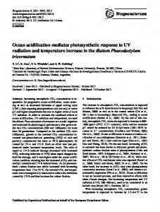
attempting to identify whether ocean acidification has, or does not have, a significant impact on a given process, this second issue can be vitally important. The unfortunately common practice of concluding that a non-significant statistical test means the treatment had no effect is both philosophically and statistically flawed: a non-significant result means that the results are inconclusive (see e.g. Nakagawa & Foster, 2004). In most routine statistical testing, the probability that an experiment does not detect a biologically important effect when such an effect is actually present (a Type II error, C) is uncontrolled and depends on sample size, variability between experimental units, the size of the actual treatment effect and the prescribed level of Type I error (B, the significance level used to reject or not reject a null hypothesis, conventionally set to 0.05). Consequently, the statistical power of the test (1 - C) is also usually unknown and variable, and the test of the null hypothesis may be weak. Importantly, we are often unaware of this. This process can be addressed using “power analysis”. This allows us to calculate the power of a test as a function of sample size for a given level of variance (obtained from pilot experiments), B, and the known, or expected, effect size. Several readily available and simple tools can calculate (for a given effect size, B, and variance) the sample sizes required in order to reject the null hypothesis with a known level of statistical confidence (i.e. power; the example given in Figure 4.1 was calculated using G*power 2). This is a valuable technique that allows us to use preliminary data to optimise the power of our experiments, thereby maximising our research outcomes per unit of research resources. Power analysis of data from pilot experiments is strongly recommended before planning definitive experiments. It is often recommended that interpretation of non-significant results be resolved using post hoc power analysis. This allows us to assess retrospectively the likelihood that our experiment could have detected a biologically important effect had it been present (see e.g. Havenhand & Schlegel, 2009). Several authors have recommended against this approach, however, because Type I and Type II error rates are non-independent, and the power of a nonsignificant test is always limited (see Nakagawa & Foster (2004) and references therein). For non-significant results, Nakagawa & Foster (2004) recommend alternative approaches for interpretation, but it is important to remember that we cannot ascribe a conclusion to lack of statistical significance: non-significant results are inconclusive. 4.4

Statistical analyses

4.4.1

Estimating variance reliably

Most commonly used statistical tests require that we make assumptions about the distribution(s) of the data in our samples, and about patterns of residual (unexplained) variance. If our data do not meet these assumptions we run the risk of introducing error that can bias the test results and lead us to inappropriate conclusions. Consequently, it is accepted practice to check assumptions about distributions of data before proceeding to use statistical tests, and there are many standard methods in commercial statistics software for doing this. Many authors move straight to formal tests of assumptions (e.g. homoscedasticity, normality) without first visually inspecting the data, yet visual representations such as boxplots (Figure 4.2) can reveal important information about underlying patterns in the data. Moreover, boxplots provide a simple yet effective alternative to formal tests of the assumptions of the intended statistical tests (Quinn & Keough, 2002). This approach is strongly recommended. If we follow a process common in the literature and choose to test formally the raw data shown in Figure 4.2 (rather than inspect the boxplots), we find that the variances in these subgroups are significantly different (i.e. heteroscedastic, Levene’s test, F5,30 = 5.3, P = 0.001) and therefore do not meet the assumptions of the ANOVA test that we might otherwise use to analyse these data. After transforming the data (using arc-sine transform) there is no significant heteroscedasticity, and the subsequent ANOVA shows a significant effect of Experiment and pH but no interaction between the two. This seems a perfectly satisfactory result, and indeed we have followed good analysis practice. 2

72

see http://www.psycho.uni-duesseldorf.de/aap/projects/gpower/

Figure 4.1 Power as a function of sample size. Pilot data are for effects of 0.4 pH unit drop on sperm motility in the mussel Mytilus edulis. A sample size of >8 males would achieve adequate power (≥ 0.8; conventionally accepted to be desirable, see Quinn & Keough (2002)). (Renborg & Havenhand, unpubl.).

As an alternative we could use boxplots to inspect the raw data visually (Figure 4.2) before moving to formal testing. Here too we can see that the data are indeed heteroscedastic (some subsets have far lower variance than others - see Quinn & Keough (2002) for guidelines on when to accept or reject assumptions of equal variance), and we would probably still choose to transform the data as before, check with a new boxplot, and then perhaps test using ANOVA in which we would of course obtain the same overall result as before. However the boxplots also show patterns that formal tests of heteroscedasticity do not reveal: the response in low pH treatments was far more variable than in high pH treatments (Figure 4.2). This finding may be at least as interesting biologically as the fact that the low pH treatments all have lower responses, yet we would have missed this if we had followed the first methodology. This highlights the value of visual inspection of data by (for example) boxplots as an important precursor to formal testing. Once we have fitted a model (ANOVA for example), visual inspection of patterns of residuals (departures from fitted models) can be very informative for detecting problems with distributions, outliers and influential values in our statistical modelling. Again, these can often reveal unexpected patterns in our data that have significance for the process under study and/or our experimental protocols. 4.4.2

Linear models – Analysis of Variance (ANOVA)

Linear models relate a single response (or dependent) variable to one or more predictor (independent) variables by estimating, and testing hypotheses about, model parameters (coefficients) for each predictor. As in the previous example, general linear models assume that response variables are normally distributed, with equal variances in the response for different levels of the predictor(s). By convention, linear models where the predictor(s) are categorical (grouping variables) are termed ANOVA models whereas those where the predictors are continuous are termed regression models. Statistically, however, these are both simply linear models and fitted in the same way using ordinary least squares (OLS). Models with both categorical and continuous predictors are also common. In contrast, generalised linear models allow distributions other than normal to be used, such as binomial and Poisson, and are based on Maximum Likelihood (ML) estimation, rather than OLS. 73

Part 2: Experimental design of perturbation experiments

Figure 4.2 Boxplot showing effects of acidification on larval development in three replicate experiments. Note that not only does acidification reduce the mean response, but also increases the variance in response (Havenhand & Williamson, unpubl.).

For ANOVA models, whether the predictor variable (often termed “factor”) is fixed or random can have an important influence on the form of the linear model, and on the form and power of the tests of our hypotheses. Many of the factors that we choose in our experiments (e.g. temperature, p(CO2), pH) are “fixed” because we determine these; i.e. we choose the levels of these factors, and we are generally not interested in extrapolating our findings to other levels of this factor. If we were to repeat the experiment we would probably choose the same levels of these factors. In a fully factorial ANOVA involving replicate independent observations of the effects of two fixed factors (say, temperature and pH) on a response variable, we determine the significance of the variance attributable to each factor, (and to the interaction between them), by comparing the variance for each of these with the variance for the residual (the only random term in the analysis). In practice this is done by generating variance ratios (“F-ratios”) using the mean-squares from the ANOVA (Table 4.3). This is a common analysis, with which most readers will be familiar. In contrast, factors are “random” when we choose a random subset of all possible levels of the factor for analysis. Random factors might be different field sites, populations, or individuals and essentially represent a level of replication. We choose these factors because we wish to make inferences about all possible levels of this factor (e.g. all individuals within a population). If we were to repeat the experiment we would use different levels. Often in biology, and especially in ocean acidification research, experiments use a mixture of fixed and random factors. In these “mixed models”, tests of the fixed factor use the interaction mean-square (rather than the residual) as the denominator (see Quinn & Keough (2002) for a detailed explanation of the logic of this analysis). As the interaction term always has fewer degrees of freedom than the residual, this usually results in a weaker test of the null hypothesis of interest. For example, changing one of the factors in the example in Table 4.3 from “fixed” to “random” reduces the significance of the F-ratio for the remaining fixed factor (pH) in the mixed model to a non-significant value (Table 4.4). Note that nothing else in this example has changed - only the nature (and name!) of one factor - however our conclusions as to the importance of pH on this (hypothetical) process would be different. Perhaps counter-intuitively, if we wish to increase the power of the test of the fixed factor (pH in Table 4.4) we must increase the number of levels of the random factor (e.g. more individuals). This is a key issue that should be taken into consideration when designing ocean acidification experiments using fixed and random factors. 74

Table 4.3 Sample factorial ANOVA table for two fixed factors. Mean squares for all factors are tested over the MSresidual. The effect of pH is significant.

4.4.3

Factor

SS

df

MS

F calc

F

P

temp

200

3

66.7

MStemp/MSres

2

0.131

pH

300

3

100

MSpH/MSres

3

0.043

temp x pH

300

9

33.3

MStempxpH/MSres

1

0.458

residual

1200

36

33.3

Repeated measures

In many of our experiments we want to know how a given response to a treatment changes over time, and whether this differs from the equivalent response in the controls. Consequently we take repeated measurements through time from the same experimental units (mesocosms, culture containers, individuals – again, here we will use mesocosms as an example). As outlined above, these repeated measures are non-independent: a measurement from any given mesocosm is more likely to be similar to a second measurement from the same mesocosm at a later date than to a second measurement from a different mesocosm. This principle also applies to time; repeated measures from the same mesocosm that are closer together in time are likely to be more correlated than measures further apart. This non-independence is fortunately not a problem because we can use a modelling approach that deals with these correlations, such as a traditional “repeated measures” ANOVA or the more general linear mixed models approach (West et al., 2006). Methods for both these approaches are available in major statistical software packages. Again, it is important to remember that multiple (in this case repeated) measurements within each mesocosm are not true replicates of the treatment. Rather, the treatment should be replicated at the level of the mesocosm. Similarly, multiple measures within each mesocosm do not increase the power of the test of treatment effect, although they will give us a better idea of how an individual mesocosm responds over time to the treatments. Although it is sometimes essential to know how a response changes over time, (effects of ocean acidification on developmental programs, for example) in other cases the change in response over time is less important (as in selection experiments). In such cases, making multiple repeated measurements can involve substantial investment in resources, and the benefits of having that extra temporal information need to be weighed against Table 4.4 Sample factorial “mixed-model” ANOVA table for one fixed factor (pH) and one random factor (individual). Mean square for the fixed factor (only) is now tested over the MSinteraction, with the result that the effect of pH is no longer significant, (note that the MS and F-values are identical to those in Table 4.3).

Factor

SS

df

MS

F calc

F

P

individual

200

3

66.7

MSindiv/MSres

2

0.131

pH

300

3

100

MSpH/MSindivxpH

3

0.088

indiv x pH

300

9

33.3

MSindivxpH/MSres

1

0.458

residual

1200

36

33.3

75

Part 2: Experimental design of perturbation experiments

the cost in resources of obtaining it: do we really need to measure responses over time, or will measures at the start and end of the experiment suffice? If the benefit:cost ratio is low, then resources might be better directed toward reducing the sampling frequency and increasing the number of replicates within each treatment level, thereby increasing the power of the experiment. These two do not always trade off directly and the issue will not always be this simple, however the principle is nonetheless important because our ability to detect any treatment effects depends on the number of replicates, not the number of repeat observations. 4.4.4

Do you know what you want? Planned vs. unplanned comparisons in ANOVA

When designing experiments we select treatments and treatment levels that are specifically relevant to our hypotheses. For example, in a simple one-way design to investigate the effects of p(CO2) on growth of an organism we may have 5 different p(CO2) levels, for each of which we have multiple replicate culture containers from which we sample at the end of the experiment. Assuming that the resulting data meet the relevant assumptions, we would analyse them with ANOVA to determine if there was a significant effect of treatment. If we find a significant effect, we often want to know where that effect lies, i.e. which p(CO2) levels differed from which others. This is a routine question that can be answered using one of the many post hoc tests available in major statistical software packages (Tukey’s test is a reliable and widely available method, and recommended here). Philosophically, these post hoc tests are different to the initial ANOVA, which tests a global null-hypothesis of no difference between any treatment groups. In post hoc tests, however, we know there is a difference (the ANOVA has already shown us this) and the question is where is the difference. These tests address all possible pairwise comparisons to detect any and all differences among the treatment groups, and consequently tests like Tukey’s control the overall probability of a Type I error, but reduce the significance level (and therefore the power) of each individual comparison. This is an excellent exploratory tool when all treatment groups are of equal interest. In contrast to this procedure, “planned comparisons” are, as the name suggests, planned a priori. Here we are not interested in all possible contrasts among the different treatment groups, but rather in only a small number of these. For example, do responses at a high p(CO2) level differ from each of the lower p(CO2) levels? We do not know the outcome of the ANOVA when we plan these tests, (indeed the overall ANOVA result may be irrelevant to our interpretation of the data), and therefore our underlying philosophy for planned comparisons is the same as that for the ANOVA, namely testing specific null-hypotheses. Planned comparisons use the sums of squares from an ANOVA to test the specific contrasts that we are interested in, and are more powerful than their post hoc counterparts. It is important however that we restrict the number of comparisons we make - the individual contrasts should be independent of each other, and therefore they should represent only a few of all possible comparisons from among the treatment groups within the data set. Again, these tests are available in most major statistical software packages, and more details can be found in the texts listed in recommended reading. Although this approach has not yet (to our knowledge) been used in ocean acidification research, it is an extremely powerful method to assess specific hypotheses, and is recommended. 4.4.5

Linear models – regression analyses

In many experiments the total number of possible replicates is limited (this especially, although not uniquely, arises in larger-scale mesocosm and field studies). Under these circumstances, rather than trying to balance a small number of replicates against a number of categorical treatment levels, a viable alternative is to run each experimental unit at a different treatment level and analyse the results using a regression model. This approach has several advantages:

76

−

for smaller numbers of replicates it is a more powerful test than equivalent ANOVA-based designs (Cottingham et al., 2005);

−

it allows identification of the functional relationship between the treatment variable (e.g. p(CO2)) and the response variable (such relationships are extremely valuable for modellers);

−

it allows prediction of responses at interpolated values of the treatment variable.

The most commonly used regression model (Model I or “y on x”) assumes that the independent or predictor variable (e.g. p(CO2)) has no error, i.e. is a “fixed” factor3. This is an important assumption if we wish to predict responses to different values of the independent variable, yet in practice the independent variable can often be subject to substantial error. Moreover, if we wish to describe the relationship between an independent and dependent variable (rather than predict the latter from the former) then a Model II (or “Geometric Mean”; “GM”) regression should be used. These Model II regressions always have steeper slopes than Model I regressions (the slope of the Model II regression is equal to that of the Model I regression divided by the correlation coefficient) and the difference between the two models increases as the relationship between the two variables becomes weaker (see Legendre & Legendre (1998) for more detail and examples). An example of the value of regression-style analyses comes from the dynamics of many biological and developmental processes. Using single time-point observations of the effects of ocean acidification on rate processes (e.g. development, population growth) can give false impressions of reduced (vs. merely delayed) response if inappropriately interpreted (Figure 4.3; Dupont & Thorndyke, 2008). An alternative approach is to follow the whole process by making multiple observations over time and then analysing the data using regression models appropriate to the process (e.g. logistic growth). Note, however, that when using this approach the experimenter must be careful to ensure that measures over time are independent, or else incorporate the non-independence (correlations structure) into the model (see section 4.4.3). The regression approach also has some drawbacks. Perhaps the greatest of these is that single values can have a strong influence on the relationship when the number of samples (points) is low. In such circumstances we must be especially vigilant to use one of the many available tools to investigate the influence of residuals. Secondly, the regression models most commonly used assume a straight-line response between the predictor (treatment) and response variable. Naturally this should always be checked by scatterplots and/or inspection of residuals. Curvilinear relationships can be modelled using non-linear models (e.g. Widdicombe et al., 2009), or transformations may be used to linearise the data. 4.4.6

Multivariate analyses

When we wish to fit models to multiple response variables, or simply wish to explore patterns in multi-variable datasets, then multivariate analyses are appropriate. These methods generally create a smaller subset of variables that each represent a combination of the original variables by maximising explained variance (e.g. multivariate analysis of variance [MANOVA] and the closely related discriminant function analysis and principal components analysis [PCA]) or calculate measures of dissimilarity between units based on the multiple variables (e.g. multidimensional scaling [MDS] and related hypothesis testing methods [e.g. ANOSIM, Permanova]). At the time of publication very few ocean acidification studies report using multivariate analyses. This is surprising because multivariate techniques in general are ideally suited to studies where multiple response variables are measured in the same experimental units (e.g. Dupont et al., 2008; Widdicombe et al. 2009). These analyses provide highly informative graphical displays and can test complex hypotheses about group differences (analogous to ANOVA) and relationships between variables (analogous to correlation/regression). Importantly, these techniques also avoid the inherent problems of increased Type I error rates that arise from multiple testing of separate variables from the same replicate units (e.g. Hall-Spencer et al., 2008). In one of the few available examples, Dupont et al. (2008) assessed the impact of ocean acidification on larval development of the brittlestar Ophiothrix fragilis, using several morphometric parameters. Each parameter was analysed individually by ANOVA and some differences were spotted, however by using a multivariate approach (Discriminant Function Analysis; Figure 4.4), larvae of different ages could be compared among treatments using all measured parameters. This led to the conclusion that low pH does not only induce a delay in development / reduced growth (see Figure 4.3 for differences in interpretation) but that larvae reared at pH 7.7 possessed proportions 3

Model I regression is the standard regression model in almost all statistical and data management packages

77

Part 2: Experimental design of perturbation experiments

Figure 4.3 The apparent effects of a treatment on a response will depend on whether measurements are made at a given time (Conclusion 1), or a given level of response (Conclusion 2). The interpretations arising from these two approaches are very different. (Adapted from Dupont & Thorndyke (2008)).

that were never observed in those reared at normal pH (8.1). This conclusion could not have been reached using univariate analyses such as ANOVA. In a broader ecosystem context, community-level analyses using multivariate (multi-taxa) techniques such as MDS and PERMANOVA are relatively simple using commercially available software (notably PRIMER™, although some analyses are also possible in “R”) and we recommend this approach strongly for any studies attempting to understand emergent ecosystem-level responses to ocean acidification (see Widdicombe et al. (2009) for an example).

Figure 4.4 Ophiothrix fragilis. Discriminant Function Analysis of morphometric parameters of larvae of different ages (d since fertilisation) and pH treatments. Coloured symbols correspond to larvae at day 3. Green is control (pH 8.1), yellow and red are low pH treatments (pH 7.9 and pH 7.7, respectively). Grey symbols correspond to the different days (from 1 to 8) in the control (from Dupont et al. (2008)).

78

4.5

Recommended texts for further reading

This section has provided some basic guidelines. We strongly encourage the reader to delve a little deeper into at least one of the excellent texts available on this topic. Ford, E. D., 2000. Scientific method for ecological research. 564 p. Cambridge: Cambridge University Press. Quinn G. P. & Keough M. J., 2002. Experimental design and data analysis for biologists. 556 p. Cambridge: Cambridge University Press. Underwood A. J., 1997. Experiments in ecology: their logical design and interpretation using analysis of variance. 504 p. Cambridge: Cambridge University Press. 4.6

Recommendations for standards and guidelines 1. General principles a) Is the design of experiments relevant to the question we intend to answer? b) What is the limit of the “sampling universe”? Is it reported correctly in the publication? Do we over-generalise the spatial or temporal applicability of our results? 2. Experimental design a) Before planning definitive experiments undertake pilot experiments and conduct power analyses to determine the required levels of replication in order to obtain adequate power. b) Minimise the risk of confounding by: − checking that observations from treatment groups are independent of each other; − check that treatments are replicated at appropriate spatial and temporal scales (avoid “pseudoreplication”); − allocate replicates to treatments randomly. c) Maximise the power to detect differences in response between treatment levels by increasing the number of replicates (experimental units to which the treatments are applied, e.g. mesocosms). 3. Statistical analyses a) Whenever possible, perform power analysis on pilot data to ensure the experimental design has sufficient statistical power, before conducting the main experiment. [NB post hoc power analysis to interpret non-significant results is not recommended]. b) Prior to formal statistical analysis, inspect patterns of variability in the raw data visually, using e.g. boxplots -- check assumptions about the distribution before proceeding to use statistical tests. c) For mixed ANOVA models, the power of the test of the fixed factor (e.g. pH, temperature) can only be improved by increasing the number of replicates of the random factor (e.g. individual). d) When possible, choose the more powerful hypothesis-driven planned comparison rather than their post hoc counterparts. e) Regression models may provide more powerful (and more broadly useful) tests -- especially when number of replicates is limited. f) Consider using statistically informative multivariate techniques to analyse experiments that measure multiple response variables from the same experimental units.

4.7

References

Berge J. A., Bjerkeng B., Pettersen O., Schaanning M. T. & Øxnevad S., 2006. Effects of increased sea water concentrations of CO2 on growth of the bivalve Mytilus edulis L. Chemosphere 62:681-687. Carpenter S. R., Kitchell J. F., Hodgson J. R., Cochran P. A., Elser J. J., Elser M. M., Lodge D. M., Kretchmer D., He X. & Vonende C. N., 1987. Regulation of lake primary productivity by food web structure. Ecology 68:1863-1876. 79

Cottingham K. L., Lennon J. T. & Brown B. L., 2005. Knowing when to draw the line: designing more informative ecological experiments. Frontiers in Ecology and the Environment 3:145-152. Dupont S., Havenhand J., Thorndyke W., Peck L. & Thorndyke M., 2008. Near-future level of CO2-driven ocean acidification radically affects larval survival and development in the brittlestar Ophiothrix fragilis. Marine Ecology Progress Series 373:285-294. Dupont S. & Thorndyke M. C., 2008. Ocean acidification and its impact on the early life-history stages of marine animals. In: Briand F. (Ed.), Impacts of acidification on biological, chemical and physical systems in the Mediterranean and Black Seas, pp. 89-97. Monaco: CIESM. Engel A., Zondervan I., Aerts K., Beaufort L., Benthien A., Chou L., Delille B., Gattuso J.-P., Harlay J., Heemann C., Hoffmann L., Jacquet S., Nejstgaard J., Pizay M.-D., Rochelle-Newall E., Schneider U., Terbreuggen A. & Riebesell U., 2005. Testing the direct effect of CO2 concentration on a bloom the coccolithophorid Emiliania huxleyi in mesocosm experiments. Limnology and Oceanography 50:493-507. Gazeau F., Quiblier C., Jansen J. M., Gattuso J.-P., Middelburg J. J. & Heip C. H. R., 2007. Impact of elevated CO2 on shellfish calcification. Geophysical Research Letters 34, L07603. doi:10.1029/2006GL028554. Gurevitch J., Curtis P. S. & Jones M. H., 2001. Meta-analysis in ecology. Advances in Ecological Research 32:199-247. Hall-Spencer J. M., Rodolfo-Metalpa R., Martin S., Ransome E., Fine M., Turner S. M., Rowley S. J., Tedesco D. & Buia M.-C., 2008. Volcanic carbon dioxide vents show ecosystem effects of ocean acidification. Nature 454:96-99. Havenhand J. N. & Schlegel P., 2009. Near-future levels of ocean acidification do not affect sperm motility and fertilization kinetics in the oyster Crassostrea gigas. Biogeosciences 6:3009-3015. Havenhand J. N., Buttler F.-R., Thorndyke M. C. & Williamson J. E., 2008. Near future levels of ocean acidification reduce fertilization success in a sea urchin. Current Biology 18:R651-R652. Hurlbert S. H., 1984. Pseudoreplication and the design of ecological field experiments. Ecological Monographs 54:187-211. Legendre P. & Legendre L., 1998. Numerical ecology. 870 p. Amsterdam: Elsevier. Michaelidis B., Ouzounis C., Paleras A. & Pörtner H.-O., 2005. Effects of long-term moderate hypercapnia on acidbase balance and growth rate in marine mussels Mytilus galloprovincialis. Marine Ecology Progress Series 293:109-118. Moore J. W., Ruesink J. L. & McDonald K. A., 2004. Impact of supply-side ecology on consumer-mediated coexistence: evidence from a meta-analysis. American Naturalist 163:480-487. Nakagawa S. & Foster T. M., 2004. The case against retrospective power analyses with an introduction to power analysis. Acta Ethologica 7:103-108. Quinn G. P. & Keough M. J., 2002. Experimental design and data analysis for biologists. 556 p. Cambridge: Cambridge University Press. Ridgwell A., Schmidt D. N., Turley C., Brownlee C., Maldonado M. T., Tortell P. & Young J. R., 2009. From laboratory manipulations to earth system models: scaling calcification impacts of ocean acidification. Biogeosciences 6:2611-2623. Spicer J. I., Raffo A. & Widdicombe S., 2007. Influence of CO2-related seawater acidification on extracellular acidbase balance in the velvet swimming crab Necora puber. Marine Biology 151:1117-1125. Underwood A. J., 1997. Experiments in ecology: their logical design and interpretation using analysis of variance. 504 p. Cambridge: Cambridge University Press. West B., Welch K. B. & Galecki A. T., 2006. Linear mixed models - a practical guide using statistical software. 376 p. Boca Raton: Chapman & Hall/CRC. Widdicombe S., Dashfield S. L., McNeill C. L., Needham H. R., Beesley A., McEvoy A., Øxnevad S., Clarke K. R. & Berge J. A., 2009. Effects of CO2 induced seawater acidification on infaunal diversity and sediment nutrient fluxes. Marine Ecology Progress Series 379:59-75.

80