Desulfurization and Regeneration Process by Using ...

ISBN 978-1-84626-023-0 Proceedings of 2010 International Conference on Chemical Engineering and Applications (CCEA 2010) Singapore, 26-28 February, 2010

Direct gas-liquid Effective interfacial area calculation of a Turbulent Contact Absorber (TCA) Amir Shabani 1, Siamak Tavoosi Asl 2  and Bahram Hashemi Shahraki 3 1 2 3

ChlorPars Company, Tabriz, Iran

Shazand Arak Oil Refining Company, Arak, Iran

Gas Engineering Department, Petroleum University of Technology, Ahwaz, Iran

Abstract. A Turbulent contact absorber (TCA) column has been installed and operated at Petroleum University of Technology (PUT) to absorb CO2 using caustic solution. In order to survey column efficiency, calculation of mass transfer coefficients (kl, kg) and interfacial area (a) is necessary. Generally because of measurement problems, these parameters are expressed as overall mass transfer coefficient (Koga). CO2 absorption by aqueous solutions (such as caustic) is considered as chemical absorption which takes place in liquid boundary layer and the rate of absorption is a severe function of gas-liquid interfacial area. Through variation of system specifications such as caustic concentration, gas rate, liquid rate and liquid to gas ratio (L/G), which resulted from 70 practical experiments with various operating conditions, subordination of effective interfacial area was investigated; a direct predictive method based on chemical absorption was presented to calculate effective interfacial area; and best operating conditions for TCA column was concluded. The final results from practical experiments illustrated that, at low L/G ratios in absorption processes, using a TCA column whose cross sectional area and packing height is about 0.1 of same parameters in a packed column which operates at the same conditions, five times efficiency can be yielded. Keywords: CO 2 absorption, Effective interfacial area, TCA, Three phase fluidized bed

1. Introduction Gas absorption using an appropriate solution is one of the most important processes in chemical and petrochemical industries. The process is based on mass transfer through gas-liquid boundary layer. In order to obtain maximum absorption efficiency, it is necessary to utilize proper equipments to maximize gas-liquid contact. Packed and Tray columns are generally used in absorption processes; nonetheless, when absorption concerns chemical reaction, regarding reaction kinetics and Stoicheiometry, it is necessary to lower L/G ratio. Lowering L/G ratio causes canalization phenomenon which is due to dried spaces in column. Canalization severely reduces mass transfer efficiency [2]. Tray columns are not economical in such conditions. Liquid holdup is high in tray columns and when solution is valuable, increased regeneration costs will affect on total absorption cost. Turbulent contact absorbers (TCA) are new columns which utilize three phase fluidized beds. These columns are operated in fully fluidized state. Packing, having no chemical effect on absorption process, maximizes gas-liquid mixing and renewal. Gas and liquid flow counter currently and packing fill about 20% of total column height. When gas rate is increased, packing start to fluidize and in further rates, fully fluidized state is yield.



Corresponding author. Tel.: +989183672674; fax: +988612789857 E-mail address: [email protected].

1

TCA columns are used in distillation, absorption and stripping processes. Turbulency and high phase mixing in TCA column cause higher mass transfer efficiency for TCA columns in comparison with packed and tray columns. TCA columns are used in conditions where L/G ratio is to be held low. A number of models have been developed for prediction of gas-liquid contact area. The widely used Onda et al. correlation assumes the contact area cannot exceed the available packing surface area [3]. The model of Djebbar and Narbaitz [4] is a modification of the model proposed by Onda and coworkers. Bravo and Fair [5], Henriques de Brito et al. [6], Billet and Schultes [7], and Piche et al. [8] have proposed models for the prediction of gas-liquid contact area. Unfortunately, these models have been based on back-calculated areas assuming models for gas and liquid mass transfer coefficients. In addition, no model is presented to predict gas-liquid contact area in TCA columns. The present work attempts to introduce a method for calculation of effective gas-liquid interfacial area in TCA columns; meanwhile, assuming CO2 absorption using caustic solution as liquid controlling chemical absorption, thus, using two-film theory, a direct predictive method for effective interfacial area calculation is presented; afterward, system parameters were changed to investigate the effect on effective interfacial area.

2. Calculation of Gas-liquid Contact area The effective mass transfer area may be estimated using a reactive absorption system such as air-CO2caustic. The absorption system can be described using two-film theory, where the liquid phase mass transfer coefficient is corrected for the chemical reaction [9]:

1 K og a



H 1  l k g a ko a

(1)

l Where  is enhancement factor and k o is physical mass transfer coefficient.

For the case of an irreversible, pseudo first order reaction, the overall gas phase volumetric coefficient Koga may be rewritten [10]:

1 K og a



1  kg a

H D AB C B k r

(2)

a

In general, for low concentrations of sodium hydroxide (CB) and high gas velocities, the liquid phase resistance dominates and the gas phase resistance can be neglected. As a result:

K og a 

a . D AB .C B .k r H

(3)

Therefore, the effective gas-liquid contact area can be deduced using measured Koga values and values of carbon dioxide diffusion coefficients (DAB), sodium hydroxide concentration (CB), the reaction rate constant (kr), and Henry’s constant(H). a

K og a.H DCO2 .C B .k r

(4)

3. Experimental System The gas-liquid contact area was measured using a 10 cm I.D. glass air-water TCA column. Column height was 180 cm. The column was filled to a depth of 20 cm with 15 mm diameter low density plastic ball packing. The caustic flow rate was measured using a rotameter. The solution entered top of the column using a reciprocating pump and contacted with gas entering column from the bottom. The gas rate was measured using a rotameter.

2

4. Experimental Results 4.1. Caustic Concentration In two constant gas flow rates, 0.897 Kmol/hr and 1.496 Kmol/hr, and constant liquid flow rate for each experiment, caustic concentration has been varied between 0.1 and 1 Kmol/m3 and the effect on mass transfer area has been presented in Fig. 1.

Fig. 1 Effective interfacial area vs. caustic normality at constant liquid rate for each curve and gas rate of (a) 0.897 and (b) 1.498 Kmol/hr

As is seen, increase in caustic concentration, decreases mass transfer area. The process is assumed to be pseudo first order irreversible chemical reaction, thus chemical reaction rate and finally mass transfer rate is expected to increase with increasing one of the reactants, but the results do not satisfy this prospect. The phenomenon can be explained using two-film theory. CO2 and NaOH reaction takes place in liquid boundary layer. CO2 has to diffuse through gas layer and enter liquid layer to reach NaOH solution. Increasing caustic concentration causes increased viscosity in liquid phase, thus CO2 penetration in liquid phase is hardened and finally mass transfer area is decreased. Diffusivity of dissolved Carbon dioxide in water and aqueous solutions was estimated using (5) [9]. 0.93

 M 0.5 L0S.5   D  5.4  10  0.5 0.3   L .V .  6

(5)

Referring (5), diffusivity is an inverse function of viscosity. In low gas and liquid flow rates, since there is sufficient residence time, increasing caustic concentration between low (0.1N) and moderate (0.5N), increases chemical reaction rate and causes more mass transfer area. On this situation, an increase in chemical reaction rate overcomes viscosity increase, but when caustic normality is varied to 1N, the drawback of viscosity increasing in the system and decrease of diffusion coefficients is so high that even increase of liquid rate at constant gas rate cannot considerably compensate the effect of viscosity.

4.2. Gas Rate At constant caustic concentration, and constant liquid flow rate at each experiment, gas flow rate has been varied between 0.9 Kmol/m3 and 1.5 Kmol/m3 and the results are being presented in Fig. 2. Except in 1Kmol/m3 normality, at all liquid rates and caustic concentrations increase in gas rate results in more mass transfer area. Turbulency and packing movements due to higher gas flow rates cause more phase mixing and better fluidization and results in more gas-liquid interfacial area. Also it is evident that in higher liquid flow rates, because of higher L/G ratio and higher buoyancy force on packing, phase mixing takes place in better manner, therewith higher liquid flow rate results in faster surface renewal in gas-liquid boundary layer, the rapid reaction consumes much of CO2 very close to the gas-liquid interface, which makes the gradient for CO2 steeper and enhances the process of mass transfer in the liquid [12]. At 1Kmol/m3 normality, the solution's viscosity is high and chemical absorption is controlling. The viscosity drawback is so high that even increasing phase mixing through more gas rate and increasing L/G ratio can not retrieve mass transfer area decrease.

3

As seen from Fig. 2c., at low liquid rate because of sufficient residence time, gas-liquid interfacial area increases with an increase in phase mixing through gas rate addition. But at higher liquid rates there is no sufficient residence time to conquest the viscosity effect on chemical absorption process.

Fig. 2 Effective interfacial area vs. Gas rate at constant liquid rate for each curve and caustic normality of (a)=0.1, (b)=0.5, (c)=1 Kmol/m3

4.3. Liquid Rate In order to investigate liquid rate effect on gas-liquid interfacial area, at fixed caustic concentration and constant gas flow rate for each experiment, liquid flow rate has been varied in range of 1.75 to 2.6Kmol/hr and the results are presented in Fig. 3.

Fig. 3 a e vs. L, at constant G for each curve and caustic normality of (a)=0.1, (b)=0.5, (c)=1 Kmol/m3 Results obtained at both low and moderate caustic concentrations and high caustic concentration at low gas flow rate; agree with the fact; increase in liquid flow rate in an absorption column, increases gas-liquid interfacial area. In other words: an increase in liquid flow rate, increases packing buoyancy and column fluidization. It also increases surface renewal at gas-liquid boundary layer and makes CO2 gradient steeper between phases. At high caustic concentration and high gas flow rate, chemical reaction residence time is limited. Increase in solution viscosity impose a reverse effect on chemical reaction rate that even increase in liquid flow rate, L/G ratio and CO 2 gradient can not compensate.

5.

Comparison of the Experimental Effective Interfacial Area of a TCA with that of a Packed column

Here to show the superiority of a TCA to a packed column, the experimental results of this work, are compared to the data taken from PhD thesis of Dr. Bahram Hashemi Shahraki [1], who has experienced CO2

4

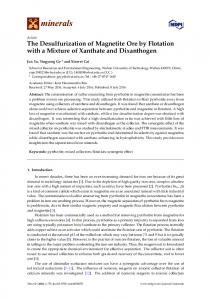
absorption using caustic solution in a packed column in the UMSIT pilot plant (1992), for a solution in the normality range of 0.1 to 1. Table II and Fig. 4 compare the effective interfacial area values measured in a TCA (this work), with those measured in a packed column by Dr. Bahram Hashemi Shahraki. The operation L/G ratio, caustic normality, column characteristics and packing shape and geometries are also given in the table for these two cases.

L/G 2.1 2.7 2.9

TABLE II COMPARISON BETWEEN PACKED AND TCA COLUMN TURBULENT CONTACT ABSORBER PACKED COLUMN NaOH NaOH a(1/m) L/G a(1/m) Concentration Concentration 244.7817 254.2053 132.2937

0.1 0.5 1

Cross sectional area= 0.14657 m2 Packing Height= 2.13m Packing size and type: dP= 38 mm, plastic pall ring

2.1 2.7 2.9

1306.272 1157.382 665.5389

0.1 0.5 1

Cross sectional area= 0.00875 m2 Packing Height= 0.2 m Packing size and type: dP= 15 mm, plastic ball

Fig. 4 Effective interfacial area vs. L/G ratio for TCA and Packed column

It is seen from the Table II and Fig. 4 that effective interfacial area in a TCA is approximately five times of the effective interfacial area in a packed bed column for the same L/G ratios and the same caustic concentrations.

6. Results and Discussion Sizeable parameters to assess TCA column efficiency are effective interfacial area (a) and mass transfer coefficients (kl, kg). Direct method for effective interfacial area calculation in TCA columns and column operating conditions has never been investigated. This work presents a direct effective interfacial area calculation method for TCA columns based on CO2 absorption using caustic solution system. The process is chemical absorption which takes place in gas-liquid boundary layer. The process is liquid film controlling. Neglecting gas phase resistance and modifying liquid phase resistance for chemical absorption, results in a direct method for effective interfacial area calculations (4). Assuming the process Isotherm and Isobar and neglecting heat production through the reaction, the sizeable parameters are limited to caustic concentration, gas flow rate and liquid flow rate. CO2 diffusivity in caustic solution is reverse function of viscosity, reaction constant (kr) is function of caustic concentration, and volumetric mass transfer coefficient (Koga) is function of gas and liquid flow rates. All these parameters were considered in calculations and results from 70 practical experiments were compared. Positive and negative effects of each parameter were estimated as follows.

6.1. Caustic Concentration Effect Basically increase in reactant amount in first order irreversible reactions, results in reaction rate increase. Regarding CO2 absorption process, diffusivity nature of the system and limited residence times, cause evident reverse effect of viscosity increase on chemical absorption process. Therefore, except in low gas and liquid flow rates, it is necessary to use thin solution.

6.2. Gas Flow rate Effect Increase in gas flow rate at studied system causes more turbulency, better phase mixing, and more mass transfer area. In the case of high solution concentration, increase in gas flow rate, causes less gas diffusion and less residence time; hence increase in gas flow rate at high solution concentration has negative effect on effective interfacial area.

5

6.3. Liquid Flow rate Effect Increasing the liquid flow rate has two advantages for the system. Firstly it results in better fluidization and phase mixing. Secondly it causes more surface renewal and more new solution is ready for CO2 to diffuse in.

7. Conclusion 

Fluidized bed columns are best choice when L/G ratio is low.



Mass transfer rate is a severe function of solution concentration and effective interfacial area.



In order to increase mass transfer resulted from effective interfacial area, regarding superiority of TCA columns (especially at low L/G ratio) liquid flow rate must be increased to highest possible extent.



In order to increase mass transfer resulted from chemical absorption, solution concentration should be increased to extent that viscosity has no reverse effect on absorption process.



In the case of low L/G ratio, through selecting the best concentration for solution, and avoiding negative viscosity effects, using a smaller column than packed columns and less packing, 2 to 5 times of mass transfer in packed columns can be accessed using TCA column.



Regarding regeneration energy costs, operation at low L/G ratio and solution consumption reduction, utilizing TCA column as a new technology, not only decreases solvent purchase cost, but also optimizes regeneration cost.

8. Acknowledgements (Use “Header1” style) We acknowledge "ChlorPars Company", "Shazand Arak oil refining company", and "Petroleum University of technology" for their technical and financial support on this paper.

9. References [1] B. Hashemi Shahraki, “CO2 absorption by caustic solution in packed and foam packed column”, PhD thesis, university of UMSIT, 1998 [2] J.M.Colson, J.F.Richardson,”Chemical engineering”, 5th ed, 2002, vol. 2, Butterworth Heinemann, pp. 675-681 [3] Onda, K., Sada, E., Murase, Y., “Liquid-side mass transfer coefficients in packed towers”, AIChE J., 5(2):235,1959. [4] Djebbar, Y., Narbaitz, R.M, “Improved correlations for mass transfer in packed towers”, Water Sci. and Tech, 38(6):295, 1988 [5] Bravo, J.L., Fair, J.R. “Generalized correlation of mass transfer in packed distillation columns,” Ind. Eng. Chem., Proc. Des. Devel. 21, 162, 1982. [6] Henriques de Brito, M., Von stoker, U., Bomio, P., “Predicting the liquid mass transfer coefficient, k1 for sulzer structured packing mellapack”, Instn. Chem. Eng. Sym Ser., 128, 1992. [7] Billet, R., Schultes, M., “Predicting mass transfer in packed columns,” Chem. Eng. Tech., 16(1), 1993. [8] Piche, S., Grandjean, B.P.A., Iliuta, L., and Larachi, F., “Reconciliation procedure for gas-liquid interfacial area and mass transfer coefficients in randomly-packed towers,” Ind. Eng. Chem. Res., 41:4911, 2002. [9] Danckwerts, P.V., “Gas liquid reactions”, 1970, New York: McGraw-Hill, pp. 276-302. [10] Robert H. Perry, Don W. Green, James O. Maloney "Chemical Engineering's Handbook", 7th ed, New York: McGraw-Hill, p. 1348. [11] Pohorecki, R. and Moniuk, W., “Kinetics of reaction between CO2 and hydroxyl ions in aqueous electrolyte solutions”, Chem. Eng. Sci., 43(7):1677, 1998. [12] Warren L. McCabe, Julian C. Smith, Peter Harriott. “Unit operation of chemical engineering”, 6th Edition, New York, McGraw-Hill, 2001.p.588.

6

ISBN 978-1-84626-023-0 Proceedings of 2010 International Conference on Chemical Engineering and Applications (CCEA 2010) Singapore, 26-28 February, 2010

Investigation of a suitable growth strategy for optimisation of intensive propagation and lactic acid production of selected strains of Lactobacillus genus M.P.Zacharof

1

, R.W. Lovitt

2

and K. Ratanapongleka

3+

1

Multidisciplinary Nanotechnology Center, Swansea University, Swansea, SA2 8PP, UK School of Engineering, Multidisciplinary Nanotechnology Center, Swansea University, Swansea, SA2 8PP, UK 3 Department of Chemical Engineering, Faculty of Engineering, Ubon Ratchathani University, Ubonratchathani 34190, Thailand

2

Abstract. Lactobacilli belong to the group of lactic acid bacteria (LAB), widely used in the food industry nowadays. These microorganisms have several distinguishing abilities such as the production of lactic acid, enzymes such as β-galactosidase and natural antimicrobial substances called bacteriocins. They are mainly used as a natural acidifier for the inoculation of bulk quantities of milk and vegetables in order to produce a variety of fermented products. As such, large quantities of their biomass and the end products of their metabolism are necessary. The possibility of producing these substances in mass quantities will be investigated through several techniques. The selected Lactobacilli, L.plantarum NCIMB 8014, L.casei NCIMB 11970, L.lactis NCIMB 8586 and L.delbruckii NCIMB 11778 were grown into simple batch cultures without pH control where their physicochemical needs were determined. Through the determination of the optimum nutritional conditions for the propagation of the Lactobacilli, an optimised medium for growth occurred. The growth efficiency on the medium was tested on a 2L STR reactor operated batch wise with continuous pH control. The optimum pH conditions for the growth of the bacilli were determined as well as parameters such as cellular yield coefficient, substrate and starter inoculum concentration and lactic acid rate and production. The metabolism of the Lactobacilli was determined as homofermentative, mainly producing lactic acid. The efficiency of the optimized medium was evaluated in terms of growth rate and doubling time through the spectrophotometric measurement of cellular biomass.

Keywords: LAB, STR, Growth rate, Doubling time, lactic acid, nutrient medium

1. Introduction Lactobacilli are a bacterial group belonging into the genre of Lactic Acid Bacteria (LAB). Their metabolic end products such as lactic acid, acetic acid, protein structure antimicrobial compounds called bacteriocins and enzymes are widely applied as food preservatives in the contemporary food industry. LAB in the form of starter cultures can be used to enhance the natural ripening of milk and plant origin products, such as butter, cheese, olives and cucumbers. Furthermore, their metabolic end products can be used as natural preservatives and antimicrobial agents against contamination and food spoilage occurring during or after the fermentation process.(2) Lactobacillus distinctive ability is to decompose complex carbohydrate sources into simpler forms and synthesise mainly lactic acid. Their use as natural acid- producer bioreactors has been widely investigated throughout the recent years, in an effort to replace the production of lactic acid from petrol and other carbon sources. (4) Furthermore, the enzymes produced from LAB have been attractively attended because these bacteria are normally  Corresponding author. Tel.: + 00447853959691 E-mail address: [email protected] Corresponding author. E-mail address: [email protected]

7

considered safe so the enzymes derived from them might be used with no need of extensive purification and there are little or no adverse effects on fermented products (1) Due to the previously referred reasons the need for bulk quantities of biomass and their end products is steadily augmenting. The research over the methods of production of enzymes, lactic acid and bacteriocins, their activity, their chemical characterisation and their extraction and their applications has to be reinforced.(5)

In this work an attempt to develop a simplified nutrient medium of low cost which will reinforce the Lactobacilli growth and lactic production has been made. Although Lactobacilli are widely applied in modern food industry their potential as natural anticiontaminants has not been deeply exploited.

2. Materials and Methods 2.1. Materials The yeast extract, peptone, glucose, lactose, Tween 80, sodium acetate, trisodium citrate, NaOH, MgSO 4 , MnSO 4 , were bought from Sigma-Aldrich Chemicals, UK.

2.2. Inoculum source All the Lactobacilli, ,Lactobacillus casei NCIMB 11970 Lactobacillus plantarum NCIMB 8014, Lactobacillus lactis NCIMB 8586 and Lactobacillus delbruckii subsp.bulgaricus NCIMB 11778 were provided in a lyophilised form by National Collection of Food and Marine bacteria(NCIMB) , Aberdeen , Scotland.

2.3. Growth Experiments 2.2.1 Preliminary Growth experiments Pyrex glass pressure tubes sealed with butyl rubber stoppers and aluminium seals were used to test the effect of basal and optimum on Lactobacilli growth. The tubes were prepared under aseptic and anaerobic conditions. The media recipe for the basal medium is glucose 2% w/v, yeast extract 1.5% w/v, peptone 1% w/v, sodium acetate, 0.5% w/v, trisodium citrate 0.2%, potassium hydrogen phosphate 0.2% w/v, MgSO4 0.02% w/v , MnSO4 0.002% w/v and resazurin dye 0.0005% v/v. The same recipe was followed for L.delbruckii although glucose was replaced with lactose, yeast and Tween 80 was added to the medium due to the extensive auxotrophic needs of the bacterium. Each component was tested separately so to certify its influence on growth in a range of concentrations between 0% w/v to 4% w/v.

All the components were combined and an optimised medium was fabricated. The medium’s recipe is glucose 2% w/v, yeast extract 2 w/v, sodium acetate, 1% w/v w/v,tri-sodium citrate 1% w/v, potassium hydrogen phosphate 0.5 w/v and resazurin dye 0.0005% v/v. For L.delbruckii, yeast extract 1%, peptone 1%, lactose 2% and Tween 80 0.1%. 2.2.2 Bench Device (Stirring Tank Reactor, STR) A 2L Pyrex glass fermenter has been selected for the procedure. The fermenter was equipped with an hydrargiric thermometer for temperature control, a pH probe (Fischer Scientific, UK) for pH control, a magnetic stir bar for agitation, an glass aeration port, a sampling and inoculation port, a gas flow stainless steel port connected with a filter for gas sterilisation (Polyvent filter, 0.2μm, Whatman Filters, UK), a port for alkali/acid feed and stainless steel coils for heat emission. All the ports were made of stainless steel and were connected with plastic tubes of several lengths. The working volume of the reactor was set at 1.5L. The pH probe was connected with a pH controller apparatus (Electrolab FerMac 260, UK) which was calibrated with suitable acidic and alkali solutions (pH 4 and pH 7) to adjust the pH range. The gas filter was connected with a gaseous nitrogen flask via rubber tubes and the flow was set up at 50 ng/ml. The alkali feed port was connected with a plastic bottle containing an alkali solution of 100 ml of NaOH 1M which was placed on an electronic scale (Ohaus portable advanced, Switzerland) o to measure the volume of alkali/acid used for pH maintenance. The coils were connected with a water bath (Grant Water bath, UK) and a pump (Watson Marlow Digital, 505S, UK) for continuous preservation of steady temperature The fermenter was placed on a magnetic stirring plate (SM1, Stuart Scientific, UK) and was constantly stirred at 150 rpm as being anaerobic bacteria

2.4. Analytical methods 2.4.1 Measurement of cellular growth and biomass

8

The cellular growth was measured by placing the pressure tubes into a spectrophotometer fitted with a test tube holder (PU 8625 UV/VIS Philips, France) at 660 nm. The tube had a 1.8 cm. light path. 2.4.2 Measurement of Lactic acid amount and rate Lactic acid productivity rate and the amount of lactic acid produced by each strain during the pH and temperature control fermentation are indirectly determined by the following theorem: 1 M of NaOH neutralises the effect of 1 M Lactic acid. According to this equation the amount of lactic acid produced is directly proportional to the amount of sodium hydroxide consumed during the fermentation process. The rate of lactic acid produced is indirectly calculated by the following equation:

dp dt

mM

/ L / h



 ( Na ) * FR * M .W .    V  

(Equation 1)

where Na is the moles of the alkali solution used, FR is the feeding rate of the alkali solution in the culture, M.W. is the molecular weight of lactic acid and V is the overall volume of the culture. (1)

3. Results and Discussion 3.1. The effect of standard and optimum medium on Lactobacilli growth Thus, to achieve the optimum maximum growth rate and of the bacteria and enhance their productivity, the bacilli were inoculated in a medium of liquid form containing all the optimised parameters. (2% glucose, 1.5% yeast extract, 0.5% potassium hydrogen phosphate, 1% tri-sodium citrate, 1%sodium acetate, lactose 2%, Tween 80 0.1%). There has been an effort to use the same parameters in the optimised medium for the inoculation and intensive propagation of all the chosen Lactobacilli., so to form a common economic simplified medium which will ameliorate distinctively the growth rates and the cellular yields of the bacteria. 1

The maximum growth rate of L.casei on the optimised medium was 0.24 h and the doubling time reduced to 2.87 h. The final biomass concentration was 2.43 g/l. When compared to the basal medium where maximum growth rate was 1 0.16 h a significant increase in the maximum growth rate was achieved. Similarly the final cell concentration of the fermentation has been raised from 1.19 g/l to 2.43 g/l. The maximum growth rate of L.plantarum on the optimised 1 medium was 0.30 h and the doubling time reduced to 2.30 h. The final biomass concentration was 2.61 g/l. When 1 compared to the basal medium where maximum growth rate was 0.13 h a significant high increase in the maximum growth rate was achieved. Similarly the final cell concentration of the fermentation has been raised from 1.32 g/l to 2.63 1 g/l. The maximum growth rate of L.lactis on the optimised medium was 0.22 h and the doubling time reduced to 3.13 h. The final biomass concentration was 1.81 g/l. When compared to the basal medium where maximum growth rate was 1 0.07 h a significant high increase in the maximum growth rate was achieved. Similarly the final cell concentration of the fermentation has been raised from 0.69 to 1.81. The maximum growth rate of L.delbruckiii on the optimised 1 medium was 0.32 h and the doubling time reduced to 2.13 h. The final biomass concentration was 3.00 g/l. When 1 compared to the basal medium where maximum growth rate was 0.20 h a significant increase in the maximum growth rate was achieved. Similarly the final cell concentration of the fermentation has been raised from 1.80 g/l to 3.00 g/l. The optimised medium will be used as a medium for further investigation. (Figures 1. 2. 3.4)

9

3

3.5

2

3

2

2

1.5

0.5

2.5

1.4

1.5

1

3.0

1.6

1

1.2

B iom a s s (g/L)

2.5

B io m ass (g /L )

2.5

B io m a s s ( g /L )

B io m a s s (g /L )

1.8

2.0

1

1.5

0.8 0.6

1.0

0.4

0.5

0.5

0.2 0 0

2

4

6

8

10

0

0 0

2

4 6 Time (h)

Time (h)

8

10

0.0

0

2

4 6 Time (h)

8

10

0

2

4

6

8

10

12

Time (h))

Fg.1. Growth of L.casei on basal Fg.2. Growth of Lplantarum on basal (□) Fg.3 Growth of Llactis on basal (□) Fg.4. Growth of L.delbruckii on basal ) and optimised (○) media and optimised (○) media and optimised (○) media and optimised (○) media

3.2. Growth of Lactobacilli on a STR In order to obtain a better maximum growth rate and higher growth yields and improved productivity a pH controlled STR system was developed. As to investigate the influence of pH over growth in terms of growth rate, doubling time and product and biomass yields the system was operated with a continuous pH control maintenance system. The influence of pH was tested in a range of highly acidic (4) to neutral (7) pH. All the process was performed in batch mode. The optimised medium was used.(3) The results of the experiments are shown in Figures 5, 6, 7 and 8. and Table 1 There is a strong correlation between the pH and the growth of the bacilli. The maximum growth rate was enhanced when the culture was controlled at pH 5.5, 6.5 and 7. Maintenance of pH on a steady state throughout the 10 h fermentation process was combined with the use of the optimised liquid medium gave highest biomass yields and maximum growth rates as compare to the uncontrolled pH growth systems. It can be also observed that on acidic pH values of 4 and 4.5, the growth of the bacilli is strongly inhibited. The amount of lactic acid produced by the bacilli was identified as being equal to the amount of NaOH used for pH maintenance. Over the 10 h fermentation the pH 5, 5.5 and 6 the bacilli were still growing as they had slower maximum growth rates and long lag periods prior to growth. Samples were measured on an hourly basis and they were analysed for biomass, pH and in some occasions the glucose and the end product were also analysed. The effect of reduced pH is strong where no growth was observed at pH 4 and pH 4.5.The optimum pH was 6.5 in the conditions studied for Lactobacillus casei NCIMB 11970 Lactobacillus plantarum NCIMB 8014, Lactobacillus lactis NCIMB 8586. Though for Lactobacillus delbruckii subsp.bulgaricus NCIMB 11778 pH 5.5 was set as the optimum pH condition. 6

9

8

5 7

6

Biomass (g/L)

Biomass (g/L)

4

3

2

5

4

3

2

1 1

0 0

2

4

6

8

10

0

12

0 Tim e (h)

2

4

6 Tim e (h)

8

10

12

Figure 7 Growth of L.lactis on Different pH range in a 2L STR,

Figure 8 Growth of L.ldelbruckii on Different pH range in a 2L STR

Growth(◊) on pH 4, Growth (□) on pH 4.5, Growth (∆) on pH 5

Growth(+) on pH 4, Growth (□) on pH 4.5, Growth (⌂) on pH 5,

Growth (x) on pH 5.5, Growth (*) on pH 6, Growth (○) on pH 6.5,

Growth (∆) on pH 5.5, Growth (*) on pH 6, Growth (○) on pH 6.5

Growth on pH 7(+)

Growth on pH 7(◊)

10

5

2.5

4.5

2

4

3

Biom ass (g/L)

Biomass (g/L)

3.5

2.5 2

1.5 1

1.5

0.5

1 0.5

0

0 0

2

4

6 Time (h)

8

0

12

10

Figure 7 Growth of L.lactis on Different pH range in a 2L STR,

2

4

6

Time (h)

8

10

12

Figure 8 Growth of L.ldelbruckii on Different pH range in a 2L STR

Growth(◊) on pH 4, Growth (□) on pH 4.5, Growth (∆) on pH 5

Growth(+) on pH 4, Growth (□) on pH 4.5, Growth (⌂) on pH 5,

Growth (x) on pH 5.5, Growth (*) on pH 6, Growth (○) on pH 6.5,

Growth (∆) on pH 5.5, Growth (*) on pH 6, Growth (○) on pH 6.5

Table 1: Lactic acid production on different pH conditions on an STR Selected Strains

pH

Rate of Lactic acid produced (mM/L/h)

Total amount of Lactic acid produced (mM)

Selected Strains

pH

Rate of Lactic acid produced (mM/L/h)

Total amount of Lactic acid produced (mM)

L.casei

4

9.94

50

L.plantarum

4

1.09

2

4.5

8.45

30

4.5

1.24

4

5

125.2

500

5

5.73

23

5.5

181.32

650

5.5

8.89

48.25

6.0

158.31

715

6.0

136.2

407

6.5

239.98

900

6.5

161.5

613

7

2.82

4

7

133.52

556

4

4.9

23

4

8.34

45

4.5

2.8

8

4.5

17.59

70

5

7.2

37

5

98.78

465

5.5

127.99

487

5.5

115.36

514

6

165.33

543

6.0

100.33

498

6.5

183.23

563

6.5

74

185

7

140.71

474.4

7

10.09

38

L.lactis

L.delbruckii

Growth on pH 7(+)

Growth on pH 7(◊)

4. Conclusions In this work, a new growth strategy to enhance lactic acid production and the growth of Lactobacilli was studied. Significant changes were notified when the optimized medium was used on the growth of Lactobacilli. Optimized pH conditions also reinforced the cellular growth and the productivity of lactic acid. Further research should be performed

11

though to develop extraction techniques for lactic acid and test further the lactic acid productivity and the nutrient media.

5. References 1.

Shimizu, K., Furuya, K., Taniguchi, M., Optimal operation derived by Green's theorem for cell-recycle filter fermentation focusing on the efficient use of the medium. Biotechnology Progress Journal 1994, 10, 258-262.

2.

Steiner, P.; Sauer, U., Long-term continuous evolution of acetate resistant , Acetobacter aceti BIotechnology and Bioengineering Journal 2003, 84, 40-44.

3.

Todorov, S. D.; Dicks, L. M. T., Influence of Growth conditions on the production of a bacteriocin by Lactococcus lactis subp. lactis ST 34BR, a strain isolated from barley beer. Journal of Basic Microbiology 2004, 44, 305-316.

4.

Van de Casteele et al., Evaluation of culture media for selective enumeration of probiotics strains of Lactobacilli and Bifidobacteria in combination with yoghurt or cheese starters. International Dairy Journal 2006, 16, 14701476.

5.

Ven Katesh K.V. Surash A.K., J. B. D., Effect of preculturing conditions on growth of Lactobacillus rhamnosus on medium containing glucose and citrate. Journal of Microbiological Research 2004, 159, 35-42.

6.

Xiao, J.; Chem, D.; Xiao, Y.; liu, J.; Liu, Z.; Wan, W.; Fang, N.; Tan, B.; Liang, Z.; Liu, A., Optimization of culture medium and conditions for a-L-arabinofuranosidase production by the extreme thermophilic eubacterium Rhodothermus marinus. Enzyme and Microbial Technology Journal 2004, 27, 414-422.

7.

Yang, S., The growth kinetics of aerobic granules developed in sequencing batch reactors. Journal of Society of Applied Microbiology 2004, 38, 106-112.

8.

Bai, D.; Jia, M.; Zhao, X.; Ban, R.; Shey, F.; Li, X.; Xu, s., L (+) - lactic acid production by pellet form Rhizopus oryzae R1021 in a stirred tank fermentor. Journal of Chemical Engineering Science 2003, 58, 785-791

12

ISBN 978-1-84626-023-0 Proceedings of 2010 International Conference on Chemical Engineering and Applications (CCEA 2010) Singapore, 26-28 February, 2010

The importance of Lactobacilli in contemporary food and pharmaceutical industry A review article M.P.Zacharof1+, R.W. Lovitt² and K. Ratanapongleka 3  1

Multidisciplinary Nanotechnology Center, Swansea University, Swansea, SA2 8PP, UK School of Engineering, Multidisciplinary Nanotechnology Center, Swansea University, Swansea, SA2 8PP, UK 3 Department of Chemical Engineering, Faculty of Engineering, Ubon Ratchathani University, Ubonratchathani 34190, Thailand

2

Abstract. Fermentation technology has been a widely researched and exploited field of the science of biotechnology. Through out the recent years the vast majority of microbial groups have been tested for the production of beneficial compounds especially for the replacement of products produced by petrol such as lactic acid. A bacterial group that heavily attracts attention due to its products are Lactic Acid Bacteria (LAB) and especially Lactobacilli. Lactobacilli are widely used in the food and pharmaceutical industry nowadays. These microorganisms have several distinguishing features based on their main ability to ferment carbohydrates such as the production of acids, enzymes and natural antimicrobial substances called bacteriocins. They are mainly used as natural acidifiers for the inoculation of bulk quantities of milk and vegetables in order to produce a variety of fermented products. As such, large quantities of their biomass and the end products of their metabolism are necessary. In this article some of the most important uses of Lactobacilli in the industry will be reviewed. Emphasis will be given in the production of lactic acid, βgalactosidase and lantibiotics through the usage of modern fermentation technology.

Keywords: LAB, fermentation technology, food industry, β-galactosidase, lactic acid,

1 Lactic Acid Bacteria and their Industrial Importance Lactobacilli are Gram positive (+) bacteria, shaped as rods which belong to the group of LAB. They are natural habitants, rapidly colonising mammalian mucosal membranes such as oral cavity, intestine and vagina In general; they are found where rich carbohydrate sources are available such as plants and materials of plant origin for example sewage and fermenting or spoiled food. (Bernardeau et al, 2006) These bacteria, in the form of starter cultures are essential for many industrial processes in the food industry, mainly for the fabrication dairy and meat products, fermentation of plants and vegetables, brewing and wine making. (Cutting, Carr, & Whiting, 1975) Lactobacilli may affect the quality, flavour, odour and texture of the final product in either a favourable or a detrimental way. (Cutting, Carr, & Whiting, 1975) The genera important members of this group are Lactobacillus, Leuconostoc, Pediococcus and Streptococcus. These organisms are heterotrophic and generally have complex nutritional requirements due to lacking of many biosynthetic capabilities. Consequently, most species have multiple requirements for amino acids and vitamins. Lactobacilli are also considered to be probiotic bacteria. Probiotics are live microorganisms that exhibit beneficial effects on the host’s health beyond inherent basic nutrition. (Rose, 1978) Lactobacilli fill in the major criteria that a microorganism should meet to be considered as a probiotic. They are surviving in a low pH environment, they are capable or surviving contact with digestive fluids and adhering to intestinal epithelial cells, they are non pathogenic to the host, they can work in multiple hosts, they have the ability of host multiplication and can easily colonise the gastrointestinal tract either permanently or temporarily and beneficially to the host and they survive in feedstuffs.Due4

  Corresponding author. Tel.: + 00447853959691 E-mail address: [email protected], [email protected]

13

to all the above abilities they are used in the production and packaging of foods (Bernardeau et al, 2006) Lactobacilli have proven to be effective against intestinal inflammation, maintenance of remission in Chron’s disease, treatment of infections during pregnancy, prevention of urinary tract infections (Ahrne et al., 2005) Lactobacilli distinctive ability is to produce lactic acid from carbohydrate sources, especially from lactose and glucose and many of them have been found to produce antimicrobial activity possessing molecules called bacteriocins. These compounds have gained major industrial interests due to their potential application to be used as natural preservatives (Rose, 1982, Board, 1983)

1.1

Application of Lactobacilli in the Contemporary Food industry Starter Cultures of Lactic Acid Bacteria (LAB)

Nowadays, LAB are constantly used in the food process industry in the form of starter cultures. Starter cultures, are carefully selected and propagated cultures of known strains of bacteria or yeasts in order to produce the suitable type of fermentation (homolactic, heterolactic, citrate etc.) .The starter cultures either consist of one pure strain of bacteria or yeasts or of a combination of strains of different microbial species.(Ross et al., 2005)As previously referred, due to their distinctive ability to produce organic acids such as lactic acid and acetic acid from carbohydrates Lactobacilli are widely applied in the food industry. These two organic acids suppress pH below the growth range causing metabolic inhibition of most pathogenic bacteria. This means that these two organic acids are among the most widely employed preservatives, used also as antimicrobial compounds. (Gruger& Gruger, 1989)

1.2

Application of Lactobacilli in Dairy Industry

Lactic Acid Bacteria (LAB) especially Lactobacilli are responsible for the formation of the microflora of most dairy products especially of cheese and fermented milk. Lactobacilli are important for flavour, colour and texture of dairy products through acidification due to lactic acid and of the metabolism of milk proteins. The most commonly used species in dairy products are L.casei, L.helveticus, L.rhamnosus, L.lactis, L.curvatus and L.plantarum. (Jack et al., 1995) Furthermore, Lactobacilli are incorporated into yogurt, cheese and fermented milk as probiotics due to their beneficial effect especially on acute and chronic inflammations of the gastrointestinal tract. (Bernardeau et al., 2006) In addition, due to the production of bacteriocins Lactobacilli also help on the preservation of dairy products. (Chen &Hoover, 2003)

1.3

Application of Lactobacilli on Wine Industry

Lactobacilli are also applied in wine industry both for grape and fruit wines, such as cider. The organic acids existing in wine which are mainly malic and tartaric acid can be easily metabolised by Lactobacilli. (Board, 1983) Malic acid is converted to lactic acid and carbon dioxide, this phenomenon is called malolactic fermentation which is extensively used for fruit wines maturation. (Liu et al., 2003) If though tartaric acid is decomposed into pyruvic and citric acid complete spoilage of the selected food product occurs. So the appropriate choice of the fermenting Lactobacilli is necessary. Usually decomposition of tartare is observed by Lactobacillus plantarum and Lactobacillus brevis (Rose, 1982)

1.4

Application of Lactobacilli on non-beverage food products of plant origin

Lactobacilli are applied in the fermentation of sauerkraut that is the product of fresh cabbage. The starter culture for sauerkraut production is the normal flora of cabbage, in addition with L.plantarum and an amount of NaCl so to avoid the growth of pathogenic bacteria. (Miller & Litsky, 1976) Another fermented product where Lactobacilli are involved is pickles. Pickles are the fermented products of cucumbers. The desirable effect is again achieved by the propagation of an L.plantarum starter culture. L.plantarum is also involved in the fermentation of olives which follows a similar pattern with the fermentation of pickles and sauerkraut, the only difference being that it is slower and involves a lye treatment. (Bernardeau et al., 2006)

2 Application of Lactobacilli in the Contemporary Pharmaceutical industry 2.1

The Production of Enzymes

Lactobacilli are well known for their role in the preparation of fermented dairy product, including yoghurt, cheese, butter, buttermilk and kefir and they are the important living bacteria in connection with lactose hydrolyzed in the present of β-galactosidase. Β-galactosidase enzyme from lactic acid bacteria have been attractively attended because this bacteria group normally considered as safe so the enzyme derived from them might be used with no need of

14

extensive purification and there are little or no adverse effects on fermented dairy products. Various strains of lactic acid bacteria have been recently researched for the enzyme for example; Strains Lactobacillus acidophilus

Researchers Comments Lin et al., 1991; Noh and Gilliland, 1993; Gupta et al., Lin, 1995; Montes et al., 1995; Wang and Sakakibara, Lactobacillus delbruckii subsp.bullgaric Ohmiya et al., 1977; Wang and Sakakibara, 1997 highest enzyme activity found about 1.5 U/cm3 Streptococcus Thermophilus Greenberg and Mahoney, 1982 Lactococcus lactis subsp.cremoris Shah and Jelen, 1991 Lactobacillus kefiranofaciens Itoh et al., 1992 Lactobacillus helveticus Wang and Sakakibara, 1997 Lactobacillus brevis Montanari et al., 2000 release the enzyme imme after the end of multiplication and is con to cell autolysis and break the cell wall Lactobacillus plantarum Fernandez et al., 1999; Montanari et al., 2000 Lactobacillus crispatus Kim and Rajagopal, 2000

2.2

The Production of Lactic acid

2.2.1 Carbohydrate Metabolism by Lactobacilli The purpose of Lactobacilli fermenting carbohydrate is primarily to achieve energy in the form of ATP capturing the primary sugar existing in the milk which is lactose. Fermentation can be described as a genre of anaerobic respiration where oxygen is not used as a final electron acceptor. In fermentation an organic molecule, in most cases a chemical intermediary accepts the electrons. In the case of Lactobacilli pyruvate is used as an electron receptor and nitrogen as an electron acceptor, being able to accept the electrons and the proton from NADH. This process is done via NAD which exists in a very small rate within the cell cytoplasm and has to be constantly regenerated so that glycolysis can continue. (Alcamo, 1997).Many circles of oxidation are required to give rapid metabolism of sugars. (Paul-Ross et al., 2002)Fermentation process can be inhibited by the Pasteur Effect which means the inhibition of glycolysis by the presence of oxygen. (Atlas & Bartha, 1993)Lactose or any other disaccharide in order to be catabolised has to be transferred into the internal of the cell. Lactobacilli use the Phosphoenolpyruvate: carbohydrate phosphotransferace system (PTS system) which is located in the cellular membrane of the bacilli. (Stanier &Gunsulus, 1961; Gerhard, 1979)Then, the primary step is the conversion of lactose into galactose and glucose. This is done by the enzyme βgalactosidase which belongs to the family of oxidases and cleaves off the β-oxygen bonded attachments to galactose. (Fytou-Pallikari, 1997). In L.lactis β-galactosidase is not strongly bonded with the cell wall but it floats freely within the cell. Lactobacilli catabolise glucose to pyruvate acid by the Embden-Meyerhof (EMP) glycolytic pathway and galactose by the Leloir pathway. The pathways are connected via phosphate-6-glucose which is the final end product in the Leloir pathway and through this form can enter the glycolysis pathway and be further converted to pyruvate acid. (Davidson &Sittman, 1999) 2.2.2 Conversion of Pyruvate to Lactic Acid 

) Pyruvate acid is the anion form of pyruvic acid ( CH 3 COCOO .Is an alpha-keto acid of the keto-acid group and under the presence of the enzyme lactate dehydrogenase (LDH) and the coenzyme NAD. Pyruvate is the major end product of glycolysis. In the case of L.lactis pyruvate is converted to C H O via lactate dehydrogenase isoform (Llactate: NAD oxidoreductase). Lactate dehydrogenase oxidises the C=O and the CH-OH (carbinol) part of pyruvic acid. The C H O produced is of L-stereo isomeric form. (Board, 1983) 3

3

6

6

3

3

2.2.3 Industrial Importance of Lactic Acid ) is an important chemical substance Lactic acid or 2-hydroxypropanoic acid ( C 3 H 6 O 3 , CH 3 CHOHCOOH widely used in food industry and in pharmaceutical and cosmetics industry. (Wasewar et al., 2003).Lactic acid is a carboxylic acid with a hydroxyl group and it is considered to be an Alpha hydroxyl acid. (AHA). It has two optically isomer forms L-(+) - lactic acid and D-(-) – lactic acid and is a chiral acid (Fytou-Pallikari, 1997).The reaction of production of L- lactic acid which is the most important form biologically, is catalysed by the enzyme lactate dehydrogenase (LDH) and its isoenzymes. It has a melting point of 53 °C, though the racemic form (D/L) has a boiling point of 122°C at 12 mm Hg.

15

Lactic acid can be produced into large amounts, biotechnologically, through fermentation process performed by bacteria such Lactobacilli. Usually, the product of fermentation is a racemic mixture conglomerate mixture of D (-) and L (+) – isomers but there are also strains which produce optically pure forms of one of the stereoisomer’s. (Martau et al., 2003) Another modern application is the use of lactic acid as a monomer participating in the synthesis of biodegradable homopolymers and co-polymers, such as polylactide (Choi & Hong, 1999). For the synthesis though of such fine polymers highly purified forms of lactic acid are demanded. Most of these polymers are used in the pharmaceutics industry especially for artificial prosthesis and controlled drug delivery.Traditional recovery methods for fermentation products (crystallization, extraction with solvent, filtration, carbon treatment evaporation) have high operational cost, so other methods such as distillation and distillation simultaneously with reaction are proposed due to low cost. (Choi & Hong, 1999)

2.3

The Production of Bacteriocins

As it has been known, a great number of Gram positive (+) bacteria and Gram negative (-) bacteria produce during their growth, substances of protein structure (either proteins or polypeptides) possessing antimicrobial activities, called bacteriocins. (Beasly & Saris, 2004) Although bacteriocins could be categorised as antibiotics, they are not. The major difference between bacteriocins and antibiotics is that bacteriocins restrict their activity to strains of species related to the producing species and particularly to strains of the same species. Antibiotics on the other hand have a wider activity spectrum and even if their activity is restricted this does not show any preferential effect on closely related strains. (Reeves, 1972) In addition, bacteriocins are ribosomally synthesised and produced during the primary phase of growth, though antibiotics are usually secondary metabolites. (Beasly & Saris, 2004) Bacteriocins usually have low molecular weight (rarely over 10 kDa); they undergo posttranslational modification and can be easily degraded by proteolytic enzymes especially by the proteases of the mammalian gastrointestinal tract, which makes them safe for human consumption. Bacteriocins are in general cationic, amphipathic molecules as they contain an excess of lysyl and arginyl residues. (Rodriguez et al., 2003) They are usually unstructured when they are incorporated in aqueous solutions but when exposed to structure promoting solvents such as triofluroethanol or mixed with anionic phospholipids membranes they form a helical structure. Some peptides form loop structures due to a disulphide bridge or on a covalent loop (Moll, Korning &Driessen, 1999)Among the Gram positive (+) bacteria, the Lactic Acid Bacteria (LAB) have gained particular attention nowadays, due to the production of bacteriocins. (Ross, Morgan &Hill, 2002) These substances can be applied in the food industry as natural preservatives. The use of LAB and of their metabolic products is generally considered as safe (GRAS, Grade One). The application of the produced antimicrobial compounds as a natural barrier against pathogens and food spoilage caused by bacterial agents has been proven to be efficient. (Chen &Hoover, 2003) 2.3.1 Applications of Bacteriocins Nowadays, bacteriocins have been widely utilised especially in the field of food preservation. The use of bacteriocins in food industry especially on dairy, egg, vegetable and meat products has been extensively investigated. Among the LAB bacteriocins Nisin A and its natural variant Nisin Z has been proven to be highly effective against microbial agents causing food poisoning and spoilage. Furthermore nisin is the only bacteriocin that has been official employed in the food industry and its use has been approved worldwide (Moll, Korning & Driessen, 1999) Numerous preservation methods though, have been used in order to prevent food poisoning and spoilage. These techniques include thermal treatment (pasteurization, heating sterilisation), pH and water activity reduction (acidification, dehydration), addition of preservatives, (antibiotics, organic compounds such as propionate, sorbate, benzoate, lactate, acetate). Although these methods have been proven to be highly successful, there is an increasing demand for natural, microbiologically safe products providing the consumers wit high health benefits. (Cutting, Carr & Whiting, 1975) Bacteriocins can be applied on a purified or on a crude form or through the use of a product previously fermented with a bacteriocin producing strain as an ingredient in food processing or incorporated through a bacteriocin producing strain. (starter culture) This method though, the incorporation of a bacteriocin producing strain, has the disadvantage of the lack of compatibility between the bacteriocin producing strain and the other cultures required for fermentation. (Ross, Morgan &Hill, 2002) However, it has been proven that a bacteriocin alone in a food is not likely to ensure complete safety; especially in the case of Gram negative(-) bacteria this has been apparent. Then the use of bacteriocins has to be combined with other technologies that are able to disrupt the cellular membrane so bacteriocins can kill the pathogenic bacteria. (Daw& Falkiner, 1999, Jack et al., 1995) Bacteriocins could be combined with other antimicrobial compounds such as sodium diacetate and sodium lactate resulting in enhanced inactivation of bacteria. Bacteriocins can

16

also be used to improve food quality and sensory properties , for example increasing the rate of proteolysis or in the prevention of gas blowing defect in cheese (Board, 1983) Another application of bacteriocins is the bioactive packaging, a process that can protect the food from external contaminants. For instance the spoilage of refrigerated food commonly begins with microbial growth on the surface that reinforces the attractive use of bacteriocins being used in conjunction with packaging to improve food safety and self-life. (Ross, Morgan &Hill, 2002) Bioactive packaging can be prepared by directly immobilising bacteriocin to the food packaging or by addition of a sachet containing the bacteriocin into the packaged food, which will be released during storage of the food product. 3.3.2. Nisin Nisin is a 34 amino acid lactococcal bacteriocin, a small polypeptide of 2, 9 kDa (Todorov & Dicks, 2004). Nisin has two variants A and Z with a difference of only one amino acid on their molecular structure (Beasly & Saris ,2004)The use of nisin as a food additive is permitted in the United States(Food and Drug Administration) in the E.U. and the U.K.(Guillet,2003) Nisin can inhibit the growth of many pathogen bacteria and bacteria causing food spoilage such as Enterococcus faecalis, Escherichia coli, Lactobacillus plantarum, Lactobacillus casei, Pseudomonas aureginosa, and Staphylococcus aureus. In the dairy industry, this lactabiotic is used to prevent spore germination of Clostiridium botulinum and Bacillus cereus. Through several studies has been identified that nisin is also found in human milk and it may protect mothers from breast infections during feeding and infants from toxication due to pathogenic skin flora such as Staphylococcus aureus (Beasly & Saris, 2004) It can interact with various different microbiomolecules. Nisin binds on the membrane localised cell wall precursor lipid II, enabling efficient membrane binding and also enhancing pore formation. This means that nisin by forming short-lived pores in biological membranes thereby killing the target bacteria (cell wall lysis).Its production is strongly dependent on the pH of the nutrient medium, the nutrient sources (carbohydrates, K, vitamins, N, P) and incubation temperature. (temperature range between 20°C to 40°C optimum 30°C). The activity levels of nisin do not always correlate with cell mass or growth rate (μ) of the reduced strain.(Oliveira, Nielsen& Forster, 2005)

3 Conclusion As it has been clearly demonstrated by the above paragraphs, Lactobacilli are an important microbial group for the productions of numerous compounds. The bulk quantities of their biomass are needed in dairy industry and further research has to be performed so to enhance their potential use as natural bioreactor which can produce efficiently many products of commercial usage.

4 References [1] Carr, J. G.; Cutting, C. V.; Whiting, G. C., Lactic Acid Bacteria in Beverage and Food. 1st ed.; Academic Press LTD.: 1975; p 17-28, 233-266. [2] Itoh, K., Toba, T., Itoh, T., and Adachi, S. (1992) Properties of β-galactosidase of Lactobacillus kefiranofaciens K-1 isolated from kefir grains, Letters in applied microbiology 15, 232-234. [3] Ahrne S. et al., Lactobacilli in the intestinal microbiota of Swidish infants. Microbes and Infection Journal 2005, 7, 1256-1262. [4] Bernadeau M. Vernoux, J. P., Henri-Dubernet, S., Gueguen M., The Lactobacillus genus. International Journal of Food Microbiology 2007, 41 p 103-125. [5] Board, R. G., A Modern Introduction to Food Microbiology. 1st ed.; Blackwell Scientific Publications: 1983; p 150. [6] Rose, A. H., Economic Microbiology :Fermented Foods. 1st ed.; Academic press LTD.: 1982; p 148-189. [7] Ross, R. P.; Desmond, C.; Fitzerald, G. F.; Stantch, C., Overcoming the technological hurdles in the development of probiotic foods. Journal of Applied Microbiology 2005, 98, 1410-1417. [8] Chen, H., Hoover, D.G. Bacteriocins and their food applications. Comprehensive Reviews in Food Science and Food Safety 2003, 2, 83-97. [9] Gruger, A.; Gruger, W., Biotechnology, A Textbook of Industrial Microbiology. 1st ed.; Sunderland,Mass Sinauer Associates: 1989; p 29-108. [10] Fytou-Pallikari, A., Biochemistry. 1st ed.; Lychnos Editions: 1997; p 141-169.

17

[11] Greenberg, N. A., and Mahoney, R. R. (1982) Production and characterization of β-galactosidase from Streptococcus thermophilus, Journal of Food Science 47, 1824-1828, 1835. [12] Gupta, P. K., Mital, B. K., Garg, S. K., and Mishra, D. P. (1994) Influence of different factors on activity and stability of β-galactosidase from Lactobacillus acidophilus, Journal of food biochemistry 18, 55-65 [13] Wasewar, K. L.; Pangakar, V. G.; Hessink, A.; Versteeg, B., Intensification of enzymatic conversion of glucose to lactic acid by reactive extraction Chemical Engineering Science Journal 2003, 58, 3385-3393. [14] Montanari, G., Zambonelli, C., Grazia, L., Benevelli, M., and Chiavari, C. (2000) Release of β-galactosidase from Lactobacilli, Food Technol. Biotechnol. 38, 129-133. [15] Montes, R. G., Bayless, T. M., Saaedra, J. M., and Perman, J. A. (1995) Effect of milks inoculated with Lactobacillus acidophilus or a yogurt starter culture in lactose-maldigesting children, Journal of Dairy Science 78, 1657-1664. [16] Noh, D. O., and Gilliland, S. E. (1993) Influence of bile on cellular integrity and β-galactosidase activity of Lactobacillus acidophilus, Journal of Dairy Science 76, 1253-1259. [17] Ohmiya, K., Ohashi, H., Kobayashi, T., and Shimizu, S. (1977) Hydrolysis of lactose by immobilized microorganisms, Applied and Environmental Microbiology 33, 137-146. [18] Shah, N., and Jelen , P. (1991) Lactase activity and properties of sonicated dairy cultures, Milchwissenschaft 46, 570–573. [19] Wang, D., and Sakakibara, M. (1997) Lactose hydrolysis and β-galactosidase activity in sonicated fermentation with Lactobacillus strains, Ultrasonics Sonochemistry 4, 255-261. [20] Liu, S.Q. (2003). Practical implications of lactate and pyruvate metabolism by lactic acid bacteria in food and beverage fermentations. International Journal of Food Microbiology, 83, 115-131 Stanier, R.Y., Adelberg, E.A., & Ingraham, J.L. (1977). General Microbiology (4th ed.): Oxford, Macmillan Press pp:496-504.

18

ISBN 978-1-84626-023-0 Proceedings of 2010 International Conference on Chemical Engineering and Applications (CCEA 2010) Singapore, 26-28 February, 2010

Study on the Antibacterial Activity of Immobilized Antibacterial Peptides on PET Nonwoven Fabrics Limei Hao1,2, Shuang Wang2, Lili Hou2, Jinhui Wu1,2, Jingquan Yang1,2+ 1 Institute of Medical Equipment, The Academy of Military Medical Sciences. Tianjin. P.R.China. 300161 2 National Bio-protection Engineering Center. Tianjin. P.R.China. 300161

Abstract. Two novel antibacterial protective materials (abbr. Peptide-PET) were prepared by immobilizing antibacterial peptides (Protamine sulfate and Polymyxin sulfate) on polyethylene terephthalate (PET) nonwoven fabrics in this study. Surface modifications of the fabric were performed via chemically modified procedure: creating carboxyl groups onto PET surface, grafting coupling agent and immobilizing the Protamine sulfate or Polymyxin sulfate. Scanning electron microscopy (SEM) was used to analyze the surface morphology of the fabrics, Toluidine blue method and X ray photoelectron spectroscopy (XPS) method were used to evaluate grafting densities. The antibacterial activities of the two Peptide-PET fabrics were investigated by Liquid Droplet Method. The SEM pictures showed that there were not any changes on the surface of the blank fabrics and modified fabrics. The results of XPS confirmed that Protamine sulfate and Polymyxin sulfate were successfully grafted on the surface of PET fabrics. The results of antibacterial experiments showed that both of them had excellent antibacterial activity against Escherichia coli and Staphylococcus aureus.

Keywords: PET Nonwoven Fabrics, Protamine sulfate, Polymyxin sulfate, Immobilization, antibacterial efficiency.

1. Introduction Antibacterial Peptides are important components of the natural defences to most living organisms. They are relatively small, cationic and amphipathic peptides of variable length, sequence and structure. During the past years, many antibacterial peptides have been isolated from animals, plants, bacteria and fungi[1], nevertheless only a few antibacterial peptides have been applied commercially, such as protamine sulfate, polymyxin sulfate et al. Protamine was found in salmon spermatozoan nuclei (salmine), it was composed of 32 amino acids in which arginine counts most. Protamine has a broad antimicrobial spectrum against bacteria and fungi and it is nontoxic to humans. All these merits make it a promising biological alternative to chemical preservatives and disinfectants[2]. Polymyxin E is a naturally occurring cyclic decapeptide isolated form Bacillus polymyxa subsp.colistinus. Polymyxin is bactericidal to gram-negative bacteria whose target site is bacterial outer cell envelope. It increases permeability of the cell envelope which lead to the leakage of cell contents, and subsequently, cell death[3]. Some researchers have combined these two antibacterial +

Corresponding author: Jingquan Yang. Tel: +086-022-84657488; Fax: +086-022-84656803.

E-mail address: [email protected].

19

peptides with materials to attain certain aims. For example, Polymyxin B was immobilized on fiber and used to cure Septic Shock after Aortic Replacement[4,5]. It also has been reported that a cellulose fiber containing immobilized protamine can be used to remove extracorporeal heparin[6,7]. Although both of them have been applied to immobilize on materials, rare reports have focused on antibacterial material field. Polyethylene terephthalate (PET) nonwoven fabric is ordinary protective material which naturally bears, reactive chain-ends on their surface, i.e. carboxyl and hydroxyl groups. These could be activated by suitable reaction with carbodiimide and tosyl chloride respectively, followed by coupling with antibacterial substances[8] . In this study protamine sulfate and polymyxin sulfate were immobilized respectively on the surface of PET fabric via chemically modified procedure as described below. These surface modified PET fabrics were characterized by Scanning Electron Microscopy (SEM) measurements and X ray photoelectron spectroscopy (XPS), and the antibacterial activity of immobilized protamine sulfate and polymyxin sulfate PET fabrics was investigated by Liquid Droplet Method.

2. Material and Method 2.1. Bacteria and agents Escherichia coli(8099) and Staphylococcus Aureus(ATCC 6538) used in antibacterial test were purchased from Institute of microbiology and epidemiology of Beijing. Nutrient broth media was used to culture bacteria. Protamine sulfate was purchased from Sigma Corporation; Polymyxin E sulfate was provided by Bio-chemistry Corporation of Zhejiang. Thermal calendaring PET nonwoven fabric was 60 g/m2 which was provided by Heng Guan Nonwoven Fabric Corporation of Tianjin. Other agents are all analytically pure.

2.2. Preparation of P 1 -PET and P 2 -PET fabrics

Surfaces of PET fabrics were modified according to the method reported by Boxus T and Chollet C[8,9], and the carboxyl groups were introduced to the surface of the PET fabrics (abbr. C-PET). Then the carboxyl groups on C-PET fabrics were activated by EDC and NHS (abbr. N-PET). After that the fabrics were immersed in PBS buffer containing 1% protamine sulfate or polymyxin sulfate and shaken at 80 r/min at 23ºC for 24h, the fabrics were taken off and washed with PBS buffer for four times every 15 min, and then dried in air(abbr. P 1 -PET and P 2 -PET fabrics).

2.3. Surface characterization To determine the amounts of carboxyl groups on C-PET fabrics, the toluidine blue-O (TBO) method was used according to Chollet C[9]. The surface morphology of the PET, C-PET, P 1 -PET and P 2 -PET were examined by scanning electron microscopy (SEM, FEI QUANTA 200) after gold coating. The chemical composition of PET and modified PET fabrics was investigated by X-ray photoelectron spectroscopy(XPS) (K-Alpha, Thermo Fisher Scientific Ltd ).

2.4. Preparation of bacteria suspension A loop of Staphylococcus aureus or Escherichia coli taken from the slant which covered with 3～10 generations of lawn were inoculated in nutrient broth and incubated at 37°C for 18～20 h at 150 r/min. Bacterial suspension was diluted to 1×108～5×108 CFU/mL by PBS buffer for further employment.

2.5. Antibacterial test The antibacterial efficiency of P 1 -PET and P 2 -PET fabrics was measured by liquid droplet method according to NU-734-99——Evaluation Test for Bactericidal Efficiency of Lysozyme-Filter. Test samples (P 1 -PET and P 2 -PET) and blank samples(C-PET) were put in sterilized plates separately (all samples were disinfected by ultraviolet treatment before experiments). 100 μL of bacteria suspension was added to the surface of samples equably until it was thoroughly absorbed. These plates were placed in thermostatic and humidistatic chamber for another 24 h, keeping temperature at 23ºC and relative humidity at 40%～60%. Then some of the samples were immersed in a 100 mL of flask containing 20 mL PBS and shaken for 2 min at 300 r/min to separate bacteria from the samples. For test samples, 100 μL of eluent were coated on nutrient

20

agar medium directly. For control samples, 100 μL of eluent which was beforehand diluted to 101 or 102 times were coated on the media to make counts easier. Each experiment repeated three times before antibacterial efficiency(AE) was calculated as formula(1).

AE (%) 

C T C

 100% (1)

Note: C ——the average colony forming units on the blank samples T ——the average colony forming units on the test samples Furthermore, after having been contacted with bacteria for 24h, some of the C-PET and P-PETs fabrics were taken off with tweezers and the morphology of bacteria on fabrics was observed by SEM. In briefly, the fabrics were put into 48-well flat bottom microtiter plate and fixed with glutaraldehyde solutions, dehydrated in a graded ethanol series, and then coated with gold. The fabrics were examined by scanning electron microscopy[10,11].

3. results and discussion 3.1. Surface characterization In this study, chemically modified procedure was employed to modify the surface of PET fabrics, which have been often used by many researchers to attain certain aims, for example, RGD had been grafted to PET fabrics using the same modification method to induce focal contact formation, osteoblast and endothelial cell adhesion[9]. After the carboxyl groups were introduced to the surface of PET fabrics, the amounts of carboxyl groups on the surface of PET and C-PET fabrics were measured by TBO method. The carboxyl groups counts of PET and C-PET fabrics were 47.10, 230.97 nmoL/mm2 respectively according to the standard curve of TBO (Table1). The results show that the amounts of carboxyl groups on C-PET fabrics were far more than that on PET fabrics, which is similar with the results of report of Chollet C et al[9]. Theoretically, the more the carboxyl groups counts on PET surface, the more the antibacterial peptides would be immobilized. Table 1 the amounts of carboxyl groups on the surface of PET and C-PET fabrics Samples

PET

C-PET

Amounts(nmoL/mm2)

47.10

230.97

SEM was employed to investigate the surface morphology of fabrics. Fig 1 A1 represents the whole shape of PET nonwoven fabrics. It showed that there were both hot melt spots and filament configuration on the surface of PET fabrics. Figure1 A2 and A3 represented the amplified pictures of filament configuration and hot melt spot respectively. Figure1 B1 and B2 were respectively represented the amplified pictures of filament configuration and hot melt spot of the surface of C-PET. Figure1 C and Fig1 D are representatives of the P 1 -PET and P 2 -PET respectively. Obviously Figure 1 exhibits that the surface of PET, C-PET, P 1 -PET and P 2 -PET fabrics was almost the same according to SEM pictures. So it indicates that this modified method does not change the surface morphology of PET fabrics and modified PET fabrics.

21

Fig 1 the surface morphology of PET and modified PET fabrics by SEM. Note: A1 represents the whole configuration of PET fabric, A2 and A3 were the amplified pictures of filament configuration and hot melt spot of PET fabric; B1 and B2 represents the amplified pictures of filament configuration and hot melt spot of C-PET; C1 and C2 represents the amplified pictures of filament configuration and hot melt spot of P 1 -PET and D1 and D2 represents the amplified pictures of filament configuration and hot melt spot of P 2 -PET.

According to the results of XPS characterization, blank PET fabrics exhibits the expected elements as only C and O elements were detected (Figure 2a) which is the same with the research of Chollet C[12], The C1s spectrum principally shows different components in blank PET fabrics which are O-C=O, C-C/C-H, C-O. A new peak corresponding to N1s appeared on the spectra of the N-PET, P 1 -PET and P 2 -PET surfaces (Figure 2b, 2c and 2d). There are new C-N components on the C1s XPS spectra of N-PET fabric except other components mentioned in the C1s spectra of blank PET fabric. N-C=O appeared on the C1s XPS spectra of P 1 -PET and P 2 -PET fabric which indicates the antibacterial peptide was immobilized on the surface of PET fabrics. The chemical compositions calculated from the XPS high resolution spectra are shown in Table 2. After the first modification step, C-PET fabrics showed C/O ratio lower than blank PET fabrics, the decreasing of C/O ratio indicates an increase of the oxygen concentration onto PET surfaces. After NHS and antibacterial peptide grafting, Table 2 shows significant differences in nitrogen percentage for materials. We can see an increase of N percentage on Peptide-PET fabrics compared to N-PET fabrics, which further confirms the success of the graft process.

Fig 2 C1s XPS spectrum for: (a) PET, (b) N-PET, (c) P 1 -PET, (d) P 2 -PET

22

Table 2 Experimental atomic composition (%) obtained by XPS analysis after each modification step material

C

O

N

C/O

C/N

PET

78.05

21.95

-

3.56

-

C-PET

77.03

22.97

-

3.35

-

N-PET

76.11

21.25

2.64

3.58

33.78

P 1 -PET

63.55

21.94

9.63

2.90

6.60

P 2 -PET

68.08

22.11

6.05

3.07

11.25

3.2. the results of antibacterial tests Table 3 the antibacterial efficiency of PET immobilized antibacterial peptides(%) Samples

P 1 -PET

P 2 -PET

E.coli

99.99

99.99

S.aureus

99.99

99.99

Fig 3 the SEM photograph of C-PET and P-PETs fabrics after direct contact with E.coli and S.aureus. Note: a: the picture of E. coli on C-PET fabric; b: the picture of S. aureus on C-PET fabric; c: the picture of E. coli on P 1 -PET fabric; d: the picture of S. aureus on P 1 -PET fabric; e: the picture of E. coli on P 2 -PET fabric; f: the picture of S. aureus on P 2 -PET fabric.

Table 3 shows the antibacterial efficiency of Peptide-PETs when they contact with bacteria for 24h. The average antibacterial efficiency of E. coli and S. aureus exposed to the P 1 -PET and P 2 -PET fabrics were 99.99% which may be due to the low minimum inhibitory concentration (MIC) values of polymyxin sulfate and protamine sulfate, for MIC of antibacterial agents used in this research were both in the level of microgramme. Bacteria were observed in all SEM micrographs after contacting with C-PET fabrics for 24h, as shown in figure 3a and 3b. After 24h direct contact, fewer microorganisms were observed on the surface of P 1 -PET and P 2 -PET fabrics (figure 3c-3f) which proves the results of antibacterial tests. Furthermore, Potter R et al., has reported the antibacterial efficacy of native and reduced charge protamine, they found that the lowest MIC values were most frequently associated with either no charge reduction or a modest (up to

23

≤20% or four blocked Arg residues) reduction in the positively charged guanidino groups of Arg[13]. In this study, the immobilized protamine sulfate on PET fabrics has excellent antibacterial effect, it showed that the modification of N terminal of protamine sulfate has not influence on or even improve its bactericidal activity. Though it is reported that the antibacterial activity of polymyxin sulfate against gram negative bacteria is better than gram positive bacteria, the immobilized polymyxin sulfate on PET fabrics has good antibacterial efficiency against both E. coli and S. aureus which implied that the amounts of polymyxin sulfate immobilized on the surface of PET fabrics were more than its minimum inhibitory concentration (MIC) against S. aureus. For we have selected antibacterial peptide which MIC value was in the level of milligramme in our experiments, after immobilizing the peptide on the surface of PET fabric using the same procedure, the antibacterial PET fabrics has poor antibacterial activity.

4. conclusion Two novel active bio-protective materials with immobilized antibacterial peptides on the surface of PET fabrics were successfully synthesized. XPS confirmed that the antibacterial peptides had been immobilized on the surface of PET fabrics. Two kinds of bacteria were selected to perform antibacterial test which were the representatives of Gram negative bacteria and Gram positive bacteria. Results of antibacterial tests indicate that immobilized antibacterial peptides have excellent antibacterial activity.

5. Acknowledgements We gratefully acknowledge the financial support provided by National Major Science & Technology Specific Projects No. 2009ZX10004-703.

6. References [1] Reddy KVR, Yedery RD, Aranha C. Antimicrobial peptides: premises and promises. International Journal of Antimicrobial Agents, 2004, 24(6), 536-547. [2] Johansen C, Verheul A, Gram L, et al., Protamine-Induced Permeabilization of Cell Envelopes of Gram-Positive and Gram-Negative Bacteria. Applied and environmental microbiology, 1997, 63(3), 1155-1159. [3] Kwa AL, Tam VH, Falagas ME. Polymyxins: A review of the current status including recent developments. Annals Academy of Medicine, 2008, 37(10), 870-833. [4] Murakami M, Miyauchi Y, Nishida M, et al., Early Initiation of Polymyxin B–Immobilized Fiber Therapy Effective for Septic Shock after Aortic Replacement. Annals of Thoracic and Cardiovascular Surgery. 2007,13(4), 287-289. [5] Shoji H, Tani T, Hanasawa K, et al., Extracorporeal endotoxin removal by polymyxin B immobilized fiber cartridge: Designing and antiendotoxin efficacy in the clinical application. Therapeutic Apheresis and Dialysis, 2007, 2(1), 3-12. [6] Zhang YH, Singh VK, Yang VC. Poly-L-lysine amplification of protamine immobilization and heparin adsorption. Journal of Biomedical Materials Research, 1998, 42(2), 182-187. [7] Yang VC, Port FK, JAE-SEUNG KIM, et al, The use of Immobilized Protamine in removing heparin and preventing protamine-induced complications during extracorporeal blood circulation. Anesthesiology, 1991, 75(2), 288-297. [8] Boxus T, Deldime-Rubbens M, Mougenot P, et al., Chemical assays of end-groups displayed on the surface of poly(ethylene terephthalate) (PET) fabrics and membranes by radiolabeling. Polymers for Advanced Technologies, 1999,7(7), 589-598. [9] Chollet C, Chanseau C, Brouillaud B, et al., RGD peptides grafting onto poly(ethylene terephthalate) with well controlled densities. Biomolecular engineering, 2007, 24(5), 477-482. [10] Beyth N, Houri-Haddad Y, Baraness-Hadar L, et al., The effect of RGD density on osteoblast and endothelial cell behavior on RGD-grafted polyethylene terephthalate surfaces. Biomaterials, 2008, 29(31), 4157-4163. [11] Beyth N, Domb AJ, Weiss EI. An in vitro quantitative antibacterial analysis of amalgam and composite resins. Journal of dentistry, 2007, 35(3), 201-206. [12] Chollet C, Chanseau C, Remy M, et al., The effect of RGD density on osteoblast and endothelial cell behavior on

24

RGD-grafted polyethylene terephthalate surfaces. Biomaterials, 2009, 30(5), 711-720. [13] Potter R, Hansen LT, Gill TA. Inhibition of foodborne bacteria by native and modified protamine: Importance of electrostatic interactions. International Journal of Food Microbiology, 2005, 103(1), 23-34.

25

ISBN 978-1-84626-023-0 Proceedings of 2010 International Conference on Chemical Engineering and Applications (CCEA 2010) Singapore, 26-28 February, 2010

 

A New Complex Between Ortho-Ester Tetra Azophenylcalix[4]arene (TEAC) And Th(IV) Tran Quang Hieu1, Nguyen Ngoc Tuan2, Le Van Tan3 + 1

Saigon Technology University, Ho Chi Minh City, Viet Nam 2 Viet Nam Atomic Energy Agency, Da lat City, Viet Nam 3 Ho Chi Minh City University of Industry, Ho Chi Minh City, Viet Nam

Abstract. A simple, sensitive and selective spectroscopy method was developed for determination of Thorium based complex of Th(IV) with ortho-Ester Tetraazophenyl Calixarene (TEAC). A new complex between TEAC and Th(IV) was found in weak medium acid, which has the ratio 1:1, λmax = 520 nm, Beer’s law was obeyed in the range 5.0 ×10-6 –2.5×10-5 mol.L-1 of Th(IV), the limit of detection was 2.5 × 10− 6 mol.L-1 and linear regression equation was determined to be: absorbance (A) = 0,248×C(10-5 mol.L-1) + 0,02 (R2 =0,990, n =7).

Keywords: Calixarene; Thorium, Spectroscopy

1. Introduction Host-guest chemistry has quickly developed during the last decade. Based on parent compound calix[n]arene, the amounts of lager derivatives have been synthesized. Particularly, calixarene chromoionophores have long been studied as specific metal ion indicators since Shinkai and co-workers reported that calix[4]arene having one 4-(4-nitrophenyl)azophenol unit with three ethyl ester group shows a Li+ ion selectivity with respect to the UV–vis band shift [1]. The 4-(4-nitrophenyl)azo group has frequently been used in calixarene-based chromoionophores. At the azo group is usually considered to be only a chromogenic center but not a metal-chelating site; to enhance the metal-binding ability, many attempts have been made to modify their lower rim (phenolic OH groups) in azo-calix[4]arene [2,3]. Scientists have reported the complexes of azocalixarenes with Ni2+[4], Cr3+[5], Fe3+[6], Pb2+ [7,8]... However, literature about complexes of azocalixarene and rare metal ions or radioactive metal ions as well as lanthanum, thorium, uranium… has been scarce. Thorium is a radioactive element, which is useful in nuclear field. The concentration of Thorium could be determined by many methods such as UV-VIS [9,14], NAA [10,11], ICP-AES or ICP-MS [12,13]. However, these methods are complicated and costly. In this report, we introduce a new reagent which can be used to develop a simple method for determination of Thorium.

2. Experimental and Results 2.1. Reagents and materials                                                              

 Corresponding author. Tel.: + (84.8.8940390); fax: +(84.8.8946268). E-mail address: [email protected] 

26

All chemicals and solvents used were of analytical grade and used without further purification unless otherwise mentioned. Double distilled and degasified water was used throughout, nitric acid HNO3 65%, P.A; MeOH, MeCN, P.A; Pb(NO3)2, P.A; Cr(NO3)3, P.A; Ni(NO3)2, P.A; CH3COOH P.A; NaOH P.A; NaNO3, P.A Merck; Th(NO3)4.5H2O; UO2(NO3)2, La(NO3)3, Sm(NO3)3.6H2O, P.A, (IAEA). The reagent OrthoEster Tetraazophenyl Calixarene (TEAC) was synthesized. Its structure and characteristics were investigated by MS, 1HNMR, FT-IR, RAMAN and reported [7]

Fig 1. Structure of Ortho-Ester Tetraazophenyl Calixarene (TEAC)

2.2. Apparatus Absorption spectra were measured with Lambda 25 UV–visible recording spectrophotometer (USA). UV stock solutions of TEAC (2.0×10−4 M, in CH3OH) and metal nitrate (2.0×10−2 M, in H2O) were prepared. The metal ion solution was diluted 10 and 100 times to give 2.0×10−3 and 2.0×10−4 M solutions. Aliquots of metal ion solution were added to the TEAC solution, and the final concentration and composition of the solution were adjusted to the desired value by adding CH3OH +H2O (7:3 v/v).

2.3. Absorbance spectra Preparatory experiments for determining the optimum testing conditions have been done. The absorption spectra of the reagent TEAC and its TEAC–Th(IV) complex under the optimum conditions are shown in Fig.2. In the figure, curve ‘a’ and ‘b’ are the spectra of TEAC and TEAC–Th(IV) complex respectively against water blank. As the observation,, the maximum absorption peak of the reagent TEAC lies at 385 nm, corresponding π π* transition of the -N= N- bond, which are in accordance with typical diazo spectra as observed by other worker [3-8], whereas the absorption peak of the TEAC –Th(IV) complex is located at 520 nm. Hence, a very large wavelength change (λ= 135 nm) is obtained.

Fig. 2. Absorption spectra of TEAC and its Th(IV) complex at pH 4.5 conditions: (a) 2.0×10-5 mol. L-1 of TEAC solution against water blank; (b) the solution containing 2.0×10 -5 mol. L-1 of TEAC and 2.0×10-5 mol .L-1 of Th(IV) against water blank

Morever, we checked the IR spectrum of TEAC and TEAC-Th(IV), Its result showed that considerable increase in the γN=N stretched frequency absorption frequencies to 1515 cm-1 as compared to that of the parent calixarenes (1501 cm-1). This shift could be attributed to the metal-azo back bonding.

2.4. Effect of pH Th(IV) tends to form hydrate precipitate in basic solution, so TEAC-Th (IV) complex was investigated in acid solution. The absorption spectra of TEAC- Th(IV) complex was obtained in the pH range 2.5–6.0. To keep

27

the other conditions optimum, appropriate concentration (2.0 10-5 mol.L-1) of reagent TEAC and Th(IV) ion concentration (2.0 10-5 mol.L-1) were chosen. The effect of pH on the absorbance of TEAC- Th(IV) complex at 520 nm is shown in Fig. 3. As can be seen from Fig. 3, in the chosen pH range, the absorbance at 520 nm increases with acidity increment first, then reach the peak point and decreases at higher pH. The maximum absorbance of the complex is obtained in the pH range 4÷5, so pH condition of 4.5 was assumed as the best and chosen for the following experiments. Different pH values were obtained by varying the relative amounts of NaAc and HAc, and confirmed by a digital pH-meter.

Fig. 3. Effect of pH on absorbance of complex formation at 520 nm (2.0×10-5 mol.L-1 of TEAC and 2.0×10-5 mol.L-1 of Th(IV).

2.5. Effect of Th(IV) concentrations To keep the optimum acidic condition (pH 4.5, the concentration of TEAC is 2.0×10-5 mol L-1), the effect of the concentration of Th(IV) on absorbance at 520 nm was checked. As can be seen from Fig. 4, the absorption of TEAC– Th(IV) complex at 520 nm shows a continuous increase in intensity along with the augment of the Th(IV) concentration in the range of 2.5×10-6 to 15.0× 10-5 mol.L-1. In addition, Beer’s law was obeyed in the range 5.0× 10-6–2.5×10-5 mol.L-1 of Th(IV), and the limit of detection was 2.5×10− 6 mol.L-1

Fig 4. Absorption spectra of TEAC with the increasing concentration of Th (IV)×10-5M From (a)→ (n) 0.0; 0.25; 0.5; 0.75; 1; 1.5; 2; 2.5; 5; 7.5; 10; 12.5; 15 equiv

2.6. Stability and composition The absorption spectra of the reagent TEAC and Th(IV) mixture were measured periodically, we found that the absorption peak at 520 nm of TEAC –Th(IV) appeared only 10s after the addition of Th(IV) to the stock solution of the reagent TEAC, the equilibrium was attained in ca. 2 min. From these characteristics, it is proposed that TEAC could be a significant chromogenic ionophores for the recognition of Th(IV) ion, this is very beneficial in the practical application of it.

28

For the complixation ratio between the host and metal ions, the Job’s plot experiment was carried out by varying the concentration of both host and metal ions. Fig. 5 shows typical Job’s plot of TEAC-Th(IV) that were conducted at 520 nm. The result showed the maximum point at the mole fraction of [TEAC]/([TEAC]+[Th(IV)]) of about 0.5 referred to a TEAC–Th(IV) complex ratio of 1:1.

Fig. 5. Job’s continuous variation plot for [TEAC]+ Th(IV) at 520 nm ([TEAC]+ Th(IV) =2.0×10-5M)

2.7. Selectivity towards Th(IV) against other metal ions We next investigated the anti-jamming ability of reage2 nt TEAC selectivity towards Th(IV) by adding other metal ions to the TEAC solution, and their UV spectra were measured and showed in Fig. 6. Upon interaction with aqueous Th(IV) solution, the reagent TEAC experienced a marked absorption peak at 520 nm and the absorption peak at 375 nm, whereas addition of other metal ions to the solution of reagent TEAC had a little change, although their absorption intensities at 385 nm increased or decreased a slightly compared to the metal ion free reagent TEAC. This important phenomenon shows that reagent TEAC possesses good selectivity towards Th(IV) even whenUO 2 2+,Sm3+,Cr3+,Fe3+,Pb2+,Ni2+ are present.

Fig. 6. The absorption spectra of reagent TEAC and TEAC–Mn+

Th (IV) N atom O atom

Fig.7 Complex’s model of TEAC with Th(IV)

Combining data from IR spectra, UV-Vis spectra, and Hyperchem 8.0, the complexation mechanisms of TEAC and Thorium ions could be explained: A four-coordinate mode 4e of metal ions complex is proposed,

29

in which four nitrogen’s of azo constructed in the centre of compound, whose centre was occupied by ion Th(IV) and the complex’s model is showed on Fig.7 Table1.ComparisonofspectrophotometricreagentsfordeterminationofTh(IV) Reagents

Condition pH

Ratio

λmax (nm)

∆λmax(nm)

ε×104 (l.mol-1.cm-1)

References

Xylenol

4

1:1

560

130

3.8

[14]

8N HClO4

1:2

645

105

13

[14]

Sunfochlorophenol S

2.5

1:1

640

90

3.3

[14]

TEAC

4.5

1:1

520

135

2.5

This work

Arsenazo III

We also compared some reagents for Th(IV) with TEAC. These data from table 1 are showed that ∆λmax(nm) of TEAC reagent is highest, so TEAC is a good reagent for determination of Thorium by UVVIS method.

3. Acknowledgements This research was fully supported by Grant from the DAAD (Germany) and Dalat Nuclear Reseach Institude. We thank Prof. Helmut Sitzmann (Faculty of Chemistry, T U Kaiserslautern, Germany) for giving a stimulating laboratory environment.

4. References [1] C. David Gutsche. Calixarene. Royal Society of Chemistry. 1992, pp. 9-19. [2] Bernadette S. Creaven, Denis F. Donlon, John McGinley. Coordination chemistry of calix[4]arene derivatives with lower rim functionalisation and their applications. Coord. Chem. Rev. In: B.S. Creaven, et al. 2008: 2-9. [3] Karci, F.; Sener, I.; H. Delig¨oz. Azocalixarenes. 1: synthesis, characterization and investigation of the absorption spectra of substituted azocalix[4]arenes. Dyes and Pigments. 2003.59: 53-61. [4] Quanli Ma, Huimin Ma, Meihong Su, Zhihua Wang, Lihua Nie, Shuchuan Liang. Determination of nickel by a new chromogenic azocalix[4]arene. In: Q. Ma, et al. Analytica Chimica Acta. 200.439: 73-79 [5] Lilin Lua, Shufang Zhub, Xingzhong Liua, Zhizhong Xiec, Xi Yanc. Highly selective chromogenic ionophores for the recognition of Chromium(III) based on a water-soluble azocalixarene derivative. In: L. Lu, et al. Analytica Chimica Acta. 2005.535: 183–187. [6] Hasalettin DEL_IG¨OZ, Emin ERDEM. Solvent extraction of Fe3+ cation by diazo-coupling calix[4]arenes. Turk J Chem. 2000. 24: 157-163. [7] Tae Hyun Kim, Su Ho Kim, Le Van Tan, Yu Jin Seo, Sun Youn Park, Hasuck Kim, Jong Seong Kim. Transition metal ion selective ortho-ester diazophenylcalix[4]arene. In: Tae Hyun Kim, et al. Talanta. 2007. 7: 1294 -1297. [8] Le Van Tan, Duong Tan Quang, Min Hee Lee, Tae Hyun Kim, Hasuck Kim and Jong Seong Kim. Determination of lead by azocalixarene. In: Le Van Tan, et al. Bull. Korean Chem Soc. 2007. 28(5): 791-794. [9] Linfeng Rao Gregory R. Choppin and Raymond J. Bergeron. Complexation of thorium(IV) with desmethyldesferrithiocin. Radiochim. Acta. 2000. 88: 851-856 [10] Kim Thomas.The Radiochemistry of Thorium. Nation Academy of Sciences National Research Council-3004. 1982, pp. 5 [11] Frank Preusser and Haino Uwe Kasper. Comparision of dose determination of using high resolution gamma spectrometry and inductivity couple plasma mass spectrometry. Ancient TL. 2001. 19 (1): 19-24. [12] Maria Luiza, Godoy, Jose´ Marcus Godoy, Renato Kowsmann, Guaciara M. dos Santos, Rosana Petinatti da Cruz. 234 U and 230Th determination by FIA-ICP-MS and application to Uranium-series disequilibrium in marine samples. Journal of Environmental Radioactivity. 2006: 1-9. [13] Tatsuya Sekil and Koichi Oguma. Determination of Thorium in high purity Aluminum by ICP-MS after matrix removal by on-line solid phase extraction. J. Flow Injection Anal. 2001. 18(2): 140-143. [14] Kiehei Ueno, Toshiaki Imamura, K.L Cheng. Handbook of Analytical Reagents. CRC Press. 2000, pp.189-196

30

ISBN 978-1-84626-023-0 Proceedings of 2010 International Conference on Chemical Engineering and Applications (CCEA 2010) Singapore, 26-28 February, 2010

Simulation of methane adsorption on open ended single-walled carbon nanotubes S. Shokri+1 , R. Mohammadikhah2, H. Abolghasemi3, A. Mohebbi4, H. Hashemipour5, M. AhmadiMarvast6, Sh. Jafari Nejad7 1, 2, 6

Research Institute of Petroleum Industry, Tehran, Iran School of Chemical Engineering, Faculty of Engineering, the University of Tehran, Tehran, Iran 4, 5 Chemical Engineering Department, Faculty of Engineering, Shahid Bahonar University of Kerman, Iran 3, 7

Abstract. In this paper, methane adsorption on open ended single-walled carbon nanotubes (o-SWCNT) is studied using molecular dynamics simulation. A site-site potential model of so-called Leonard-Jones is considered to evaluate all interactions. Monolayer adsorption isotherms for methane inside/outside of an armchair (10, 10) o-SWCNT are obtained in different temperatures. The simulation data are compared with those of the classical adsorption models. Among the many isotherms tested for the simulations, we found that the hybrid isotherm model of the Langmuir and Sips with four parameters nicely fitted the simulation data. The isosteric heat of adsorption is measured as well. Keywords: Adsorption, Surface coverage, Isosteric heat, Langmuir equation, Monolayer, Sips equation.

1. Introduction Demand for clean fuels for vehicles of coal and petroleum has been rapidly increasing with the development and progress of modern civilization. In this regard, hydrogen and natural gas, whose main component is methane, are commonly considered to be suitable non-pollution alternatives to fossil fuel. Hence, the storage of natural gas has become an important subject. Generally, heavy steel cylinders stores the compressed natural gas under pressures up to 30 Mpa while adsorbed natural gas requires a lower pressure (e.g. about 4 Mpa) to be stored in a lightweight container. Compared to the compressed natural gas, adsorbed natural gas is a very promising because storage in lower pressures leads to lower cost and weight of fuel [1-3]. Recently, there has been a resurgence of interest in potential of carbon materials as gas storage media following claims that single-walled carbon nanotubes, SWCNTs, may have high gas storage capacities. Besides, another possible way of methane exportation can inexpensively be developed via such an adsorptive strategy. For these reasons, the methane adsorption process deserves to be more and more known. Experimental investigation of methane adsorption on closed ended single-walled carbon nanotube bundles has been carried out by Talapatra et al. [4]. Grand canonical Monte Carlo simulations with a Leonard-Jones potential have been performed to study the adsorption of methane at room temperature on triangular arrays of SWCNT [5]. Adsorption of methane on an isolated SWCNT has been investigated so as to increase the volumetric capacity [6]. Kaneko and co-workers have also been studied the methane adsorption process on SWCNT using a density functional theory method [7]. They found that SWCNT with disordered structure could be applied as storage media for methane and other supercritical gases. Information about selfdiffusivity of methane obtained from a classical molecular dynamic (MD) simulation at sub- and supercritical conditions is available [8]. To our knowledge, to date there have been no studies about investigation of the classical models for this particular process. In general, there have been a few reports on the adsorption of methane on the surface of SWCNT by means of both experiments and MD simulations. In + Corresponding author. Tel.:+989124897729; fax:+982144739713 E-mail address:[email protected]

31

this paper, methane adsorption on/in (10, 10) SWCNTs is probed at different temperatures and pressures using molecular dynamic simulations. Surface coverage for both exohedral and endohedral associated with isosteric heat is reported. Finally, the simulation data are correlated with some of the classical adsorption models looking for a suitable model for prediction of adsorption capacity.

2. Method MD calculations are carried out in the NVT ensemble by a new code written in the FORTRAN77 software environment. Both carbon atoms and methane molecules are treated as spherical rigid bodies. Pairwise interactions between fluid-fluid and fluid-surface are modeled with Leonard-Jones potential. This potential is define as below: U

lj

6     12     4        r     r 

(1 )

Where r is the separation distance between two individual bodies. The energy and size parameters of the LJ potential are ε f =148.12 K, σ f =3.81 Å for methane-methane interactions and ε f =28 K, σ f =3.35 Å for carbon-carbon interactions [9]. Lorentz-Bertholet combining rule is used for estimation of fluid-surface interactions in this form [10]:  f c (2) and  sf   3 . 58 Å 2

 sf   c  f  64.4 K

(3)

A perfect (10, 10) SWCNT with opened ends, is chosen as absorbent. Fig.1 is showing our substrate enclosed by a fictitious cubic box. Each unit of cell of the (10, 10) SWCNT comprises 40 carbon atoms with the radius and length of 6.78 Å and 2.46 Å, respectively. The substrate included 1520 carbon atoms corresponding to 38 unit cells duplicated along the tube axis. The substrate is enclosed by a cubic box of 95.2×95.2×95.2 Å3 (simulation box) as one can see in Fig.1 where the c-c bond length through the absorbent is about 1.42 Å. The number of methane molecules in the simulation box varied between 32 and 6912 molecules. Since in MD the large intermolecular potentials and the correspondingly large forces could cause difficulties in the solution of the stiff differential equations of motion, the initial configuration of methane molecules has been organized according to the face-centered cubic (fcc) structure with its 4M 3 ( M  2,3,4,5,...) lattice points. Our code incorporated an important section through which all overlaps between methane molecules and surface were eliminated until the maximum distance between fluid molecules and SWCNT is less than 0.8σ sf . This action avoids large-scale interactions. Initial linear momentums (velocities) were set by a random generation Monte Carlo method, which was satisfying the principle of total momentum conservation. Initial angular momentums were taken as zeroes, so the momentum conservation rule becomes: Nf

P   mi v i  0

(4)

i 1

A Woodcock extended system thermostat is used to rescale the velocities for fixing the kinetic temperature of the system [13]. The way is that at each time step the velocities are multiplied by a factor of (T/T curr )1/2, where T is the desired thermodynamic temperature and T curr is the current kinetic temperature. The fixed carbon atoms are not included in the calculation of temperature.

32

Fig.1: Computer-generated image of an armchair (10, 10) SWCNT.

The 3-D periodic boundary conditions were imposed on methane molecules so as to vanish the surface effect of the box faces. The LJ potential model is truncated for the Vander Waals cutoff that is chosen 12.8 Å, therefore, any interaction related to farther distance is assumed to be negligible. The system is equilibrated for 1200 ps and the ensemble averages of properties of interest are evaluated and stored during simulation. The relaxation of initial configuration to equilibrium evolves 120000 time steps. No studies in MD have reported such long time simulation because of some limitations of computer systems in addition to molecular modeling packages. However, the simulation procedure will certainly be bothersome if user uses the usual MD packages. Conversely, the use of manual codes is more convenience to handle various problems but more difficult to write. We optimized the integration time, the main section, of our program and could proceed the simulation procedure to long times. This action gives us results that are more reliable. The equations of motion in the form of Hamiltonian are integrated by the Varlet’s algorithm when the time step is short enough as 1 fs [11]. The ensemble averages obtained from simulations are taken into account for secondary analysis. A new program was linked to the main program for subsequent calculations. The uncertainties on the ensemble averages are calculated by repeated simulations and estimated to be less than 2%.

3. Results and discussion 3.1. Coverage on o-SWCNT This fact has been recognized that methane is weakly adsorbed on/in CNTs even under very high pressure (i.e. the interaction between methane-CNT is of small degree of magnitude) [15]. Results show at low pressure, a symmetrical monolayer of methane molecules is constituted around and inside of CNT. When the pressure increases, the second, third, fourth and higher layers are formed around CNT successively while inside of CNT there is only one layer. The pressure increase is equivalent to increase in methane molecules in the box. Fig.2 shows a 2-D snapshots of methane adsorbed on/in SWCNT compared to its initial configuration where the number of methane molecules, kinetic temperature and average pressure are 4000, 70 K and 3.89 Mpa, respectively. In this case, the system reaches the liquid state. From this figure, it is clear that the first, 2nd and 3rd layers are nearly complete but the higher levels are incomplete.

Fig.2: Two dimensional snapshots of (a) initial (fcc) and (b) equilibrium configurations.

The simulations are performed at different temperatures as 70, 170, 273 and 298 K under which temperatures the surface coverage changes very sensitively against the temperature variation. For example, at 298 and 273 K only monolayer is formed when the further layers are vanished. This fact is related to the increases in kinetic energy in contrast with potential energy, which is responsible for surface adsorption. The total energy, Hamiltonian, are conserved during the system evolution as long as the algebraic summation of kinetic and potential is identical to zero. In the other words, increase in kinetic energy results decrease in potential energy and vice versa. The mathematical aspect of this law is:

H U  K  0

(5)

Where H, U and K are total (Hamiltonian), potential and kinetic energies, respectively. Consequently, increases in temperature indeed decrease surface coverage. At each time step, Eq.5 has to repeatedly be checked to prevent divergence. The equilibrium distance between the CNT wall and the first monolayer of

33

methane was spanned as 3.33 Å while for internal layer it was 3.48 Å. The internal distance is found to be higher than the external distance because of the counter interactions induced by carbon atoms in the opposite site of wall. Surface coverage of methane adsorption is expressed in terms of atomic ratio of adsorbed methane to carbon by Eq.6.  

Nm Nc

(6 )

That N m stands for the number of methane molecules adsorbed on the substrate. This property may also be expressed in either volumetric or mass unit, although the atomic unit is the best choice due to its high accuracy. Surface coverage at four different temperatures is calculated under several pressures, as one can see in Fig.3. The average pressure is integrated over its instantaneous values divided to the number of time steps. 0.3

Coverage (dimensionless)

0.25 0.2 External layer (70 K)

0.15

Internal layer (70 K) External layer (170 K)

0.1

Internal layer (170 K) External layer (273 K)

0.05

Internal layer (273 K)

0 0

5

10

15

20

25

30

35

40

-0.05 Pressure (MPa)

Fig.3: Coverage of methane adsorption on the external and internal surface of the (10, 10) o-SWCNT at different temperatures.

Saturation coverage for 70, 170, 273 and 298 K are directly evaluated with counting the adsorbed molecules under high pressures and for the first external layer find to be 0.278, 0.248, 0.201 and 0.197 while for internal layer the corresponding values are 0.0253, 0.0250, 0.0230 and 0.0217, respectively. Fig.2. (a) showing that there are initially four columns of methane molecules confined inside the (10, 10), after equilibrium, methane molecules take a 2D cubic configuration. By increasing internal coverage, this structure changes from previous to a 2D hexagonal one and subsequent proceeding gives a 2D gyrate form. This fact is also observed for external layers but less sensible.

3.2. Investigation of models In this section, some of typical adsorption models whether theoretical or experimental, namely Langmuir, Sips, Freundlich and Langmuir-Sips, are correlated with the simulation data. The relations of these models accompanied by more details about can be found elsewhere [12]. For instance, the hybrid isotherm of Langmuir-Sips is defined beneath:

 bL p bS p 1 / n    qm   1/ n  1  bL p 1  bS p

  

(7 )

Where θ, the fractional coverage, is the ratio of unsaturated coverage to the full capacity of under consideration layer and p is the mean pressure of the system. Subscripts L and S denote on their belonging to the Langmuir and Sips equation, respectively. The parameters b, n and q m at specified temperature are constant values having only material dependency. Prior to start analysis, some of the doubtful simulations were repeated. Eventually, the data were carefully looked over and some of the adverse data points were rejected. However, the hybrid isotherm of Langmuir-Sips, capable of explaining the coverage of both internal and external layers, was superior to flexible fit of isotherm data than others although its physical meaning is arguable. Results for monolayer methane adsorption at 70 K are shown in Fig.4 from which the

34

excellent agreement between the hybrid model and the data is evident. This conclusion is thoroughly consistent with that obtained from analysis on experimental data [2].

Fig.4: Correlation between common models and simulation data at 70 K. The values of R-square for Langmuir, Freundlich, Sips and hybrid isotherms are 0.939, 0.802, 0.989 and 0.992, respectively. Henceforth, our attention will be focused on this isotherm because of its high accuracy. Four parameters of the hybrid model were determined by a nonlinear least squares fitting routine of the Nelder-Mead simplex method done in MATLAB software curve fitting toolbox environment. Adjusted R-square is calculated for fit plots as a criterion of precision. To better understanding of coverage behavior at different temperatures, the fitting procedure was continued, unceasingly. A comprehensive report of the outcome of the fitting is incorporated in Table.1. To our knowledge, such results are being reported for the first time since there has not been any similar work in the literature. The LangmuirSips parameters for methane adsorption on MWCNTs just corresponding to the external monolayer are available [2]. It is observable from Table.1 that all parameters change with temperature, erratically. The temperature functionality of the parameters will be unknown in that the number of data point is poor, so the curve fitting is inappropriate. The only way of finding the parameters should be the interpolation between the present data. If a theoretical definition is accessible, the functionality can be known. For example, the temperature dependency of bL or bS is hypothetically presented by this equation [12]:

bL  b0 exp(

b

E

E ads ) RT

(8)

Where 0 , R and ads are pre-exponential factor, universal gas constant and activation energy of adsorption. Eq.8 is valid for Langmuir or Sips equation, discretely, but in combination, the separation contributions of Langmuir and Sips are not transparent. We found that Table.1 and the data therein do not satisfy Eq.8 anyway. This fact is good evidence to previous claim about unknown relation between Eq.7 and Eq.8. Table.1: The parameters of Langmuir-Sips equation (Eq.7) in various temperatures. n Adjusted R-squared Layer to be studied Temperature (K) b b q L

Internal

External monolayer

70 170 273 298 70 170 273 298

S

0.034 0.017 2.764E-12 0.010 1.958 1.602 0.388 0.404

3.57E-8 2.29E-8 2.31E-7 3.07E-7 3.702 0.127 0.331 0.269

m

0.039 0.091 0.160 0.127 0.405 0.150 0.448 0.882

0.757 0.720 0.970 0.751 0.522 0.503 0.512 0.517

0.947 0.914 0.949 0.920 0.987 0.999 0.998 0.988

The thought is the essence of Eq.7 probably is different from its composer equations such as Langmuir or Sips.

3.3. Isosteric heat 35

One of the basic quantities in adsorption studies is the isosteric heat, q st , which is the ratio of the infinitesimal change in the adsorbate enthalpy to the infinitesimal change in the amount adsorbed. The information of heat released is important in the kinetic studies because when heat is released due to adsorption, the released energy is partly absorbed by the solid adsorbent and partly dissipated to the surrounding. The portion absorbed by the solid increases the particle temperature and it is this rise in temperature that slows down the adsorption kinetics because the mass uptake is controlled by the rate of cooling of the particle in the later course of adsorption. Hence, the knowledge of this isosteric heat is essential in the study of adsorption kinetics. The isosteric heat may or may not vary with loading. It can be determined from the slope of the plot of lnp versus 1/T for a fixed amount of gas adsorbed on the substrate and is given by Eq.9.

  ln p  q st   R   1 / T 

(9)

Variations of lnp with 1/T for both external and internal locations are depicted in Fig.5. The figure is presenting that the slope of the supposed straight lines is unexceptionably negative thus the isosteric heat of adsorption takes positive values in this particular case. The isosteric heat of endohedral and exohedral adsorption of methane as a function of coverage is also illustrated as one can see in Fig.6. As a consequence, this figure shows that isosteric heat of endohedral adsorption follows a piecewise manner whereas exohedral heat is fully continuous. Surprisingly, the endohedral plot shows two sharp peaks; the tallest is in vicinity of coverage of 0.02, which declines rapidly with increase in amount of coverage. Prevalently, the adsorption process is of great interest to be carried out in descending region (i.e. after the tallest peak) because the maximum amount of coverage and minimum generation of heat of adsorption is coincidently reached. For external layer, this treatment is not found.

Fig.5: Variation of lnp versus 1/T in a plenty of coverage for (a) endohedral and (b) exohedral adsorption.

Fig.6: Variation of isosteric heat against coverage for (a) endohedral and (b) exohedral adsorption.

36

Fig.6. (b) reveals that the exohedral isosteric heat increases with the coverage increase due to attractive interacting with neighbor molecules. If we had taken the higher amount of coverage into calculation, a maximum value of exohedral isosteric heat would surely have obtained due to repulsive forces among adsorbed molecules.

4. Conclusion Methane adsorption on/in SWCNTs is studied at different temperatures as well as pressures. The MD simulations are conducted in NVT ensemble (canonical ensemble) considering molecules as rigid bodies. LJ model is selected to predict all site-site interactions and energy and size parameter are estimated by LB mixing rule. Hamiltonian equations of motion are solved according to the Verlet’s algorithm for a long duration of time. Partition function and pressure of the system are evaluated as well. Surface coverage for both internal and external monolayer is directly calculated. It is found that methane molecules are weakly adsorbed on CNT. As a result, the coverage increases with pressure increase while decrease with temperature increase. The simulation data conform to those of predicted by the hybrid isotherm of Langmuir-Sips model. The parameters of the Langmuir-Sips model are obtained via fitting on the simulation data. Finally, the isosteric heat of methane adsorption is studied and it is found that this quantity increases firstly with increase in amount of coverage and decreases, afterwards. Our next work will be centralized on multilayer methane adsorption on/in SWCNTs.

5. Acknowledgment The authors would like to thank Prof A. Nasehzadeh, from the Chemistry Department, Faculty of Science, Shahid Bahonar University of Kerman, Kerman, Iran for helpful discussions.

6. References [1] H. Tanaka, M. E. Merraoui, W. A. Steele, K. Kaneko. Methane adsorption on single-walled carbon nanotube: a density functional theory model. J. Chem. Phys. Lett., 2002, 352: 334-341. [2] J. W. Lee, H. C. Kang, W. G. Shim, C. Kim, H. Moon. Methane adsorption on multi-walled carbon nanotube at (303.15, 313.15, and 323.15) K. J. Chem. Eng. Data., 2006, 51: 963-967. [3] D. Castello, J. Monge, M. A. de la Lillo, D. Amoros, A. Solano. Advances in the study of methane storage in porous carbon nanotube materials. J. Fuel., 2002, 81: 1777-803. [4] S. Talapatra, A. D. Migone. Adsorption of methane on bundles of closed-ended single-walled carbon nanotubes. J. Phys. Rev. B., 2002, 65: 1-6. [5] D. Cao, X. Zhang, J. Chen, W. Wang, J. Yun. Optimization of single-walled carbon nanotube arrays for methane storage at room temperature. J. Phys. Chem. B., 2003, 107: 13286-13292. [6] E. Bekyarova, K. Murata, M. Yudasaka, D. Kasuya, S. Iijima, H. Tanaka, H. Kahoh, K. Kaneko. Single-wall nanostructured carbon for methane storage. J. Phys. Chem. B., 2003, 107: 4681-4684. [7] H. Tanaka, El. Merraoui, W. A. Steele, K. Kaneko. Methane adsorption on single-walled carbon nanotube: a density functional theory model. J. Chem. Phys. Lett., 2002, 352: 334-341. [8] D. Cao, J. Wu. Self-diffusion of methane in single-walled carbon nanotubes at sub- and supercritical conditions. J. Langmuir., 2004, 20: 3759-3765. [9] W. Shi, J. K. Jahnson. Gas adsorption on heterogeneous single-walled carbon nanotube bundles. J. Phys. Rev. Lett., 2003, 91: 1-4. [10] M. P. Allen, T. J. Tildesley. Computer simulation of liquids. Clarendon Press, Oxford, 1990. [11] D. Frenkel, B. Smith. Understanding molecular simulations: from algoritms to applications. Academic Press, New York, 1996. [12] D. D. Do. Adsorption analysis: equilibria and kinetics. Imperial College Press, Vol.2, London, 1998.

37

ISBN 978-1-84626-023-0 Proceedings of 2010 International Conference on Chemical Engineering and Applications (CCEA 2010) Singapore, 26-28 February, 2010

A new method of exergy analysis for determination of optimum operation parameters in double- pipe heat exchangers Seyed Ali Ashrafizadeh 1, Majid Amidpour 2 1 2

Chemical Engineering Group, Islamic Azad University- Dezfoul branch Faculty of Mechanical Engineering, K. N. Toosi University of Technology

Abstract. Double- pipe heat exchangers have been evaluated in exergy analysis by combination of the thermodynamic relations, exergy concept and sink-source model. In this study some new expression for exergy losses calculation has been obtained. Since heat transfer and fluid flow friction are two sources for irreversibility in heat exchangers, exergy losses terms have been investigated, independently. Two of the most identified cases in operation parameters for heat exchangers have been discussed: (1) Optimum outlet temperature of cold and hot fluids (2) Optimum outlet temperature and flow rate for one of the fluids in the heat exchangers. The maximum and the minimum points in exergy losses have been obtained, with regards to the aforementioned cases. Keywords: exergy analysis, double- pipe heat exchanger, optimization.

1. Introduction Heat exchangers are typical in industries, especially in the chemical industry. The main goal is to either increase cold fluid temperature or to decrease hot fluid temperature or doing both simultaneously. In each case the purpose is exergy transfer from one fluid to another. Temperature difference is the driving force in heat transfer causing irreversibility and entropy generation or exergy losses. Besides that, fluid flow frictions are considered as yet another reason for irreversibility in heat exchangers. Thus it is impossible to transfer the whole exergy from one fluid to another; on the other hand, entropy generation and exergy losses are indispensable in heat exchangers. Information about these losses can be valuable in terms of optimization while ignoring them can increase the level of erroneous operation and design. The second law and exergy analysis, as suitable devices for second law application have unfortunately not been used in the heat exchanger design. Although exergy analysis is used after building the heat exchangers and pinch technology is used in net of heat exchangers, it would be more helpful to do actually do the analysis in the design phase, before building it. If second law of thermodynamics has not been considered in design phase, exergy losses can primarily only be decreased by changing the operation parameters while not changing the structure of heat exchanger. Doing this would minimize the costs. There are some basic researches about this topic: A. Bejan [1, 2] has focused on the different reasons for entropy generation in applied thermal engineering. Fraser and Mahmud [3, 4] applied the second law for analyzing the heat transfer and fluid motion in a rotating concentric cylinder. Analyzing the mechanism of entropy generation in basic configurations, they encountered eight different types of convective heat transfer problems. Sahin [5] studied the entropy generation and pumping power for a turbulent flow in a smooth pipe with constant wall heat flux. Tasnim and S. Mahmud [6] simplified the governing equations in cylindrical coordinates and solved them using isothermal boundary conditions to analyze mixed convection flow, heat transfer, and entropy generation characteristics. Eryener and Buyruk [7], experimentally studied the  Corresponding author. Tel.: +00982188677272; fax: 00982188677272. E-mail address: [email protected]

38

influence of the process variables on the exergy losses at double tube heat exchangers. P. Naphon [8] investigated the second law on the heat transfer of the horizontal concentric tube heat exchanger. M. Yilmaz, O. N. Sara, S. Karsli [9] performed evaluation criteria for the heat exchangers based on second law analysis. A. Gupta, S. K. Das [10] studied second law analysis of cross flow heat exchangers in the presence of axial dispersion in one fluid. T. H. Ko, K. Ting [11], obtained optimal Reynolds number for the fully developed laminar forced convection in a helical coiled tube. In most of the above-stated research, basic equations have been evaluated. However some simple methods seem to be needed to encourage designers and operators for exergy analysis application in initial designs and operations. The available literature shows that the exergy analysis has already been done in terms of a stream- wise model and its focus has been concentrated on inlet- outlet flows. But this article presents a simpler path with readily digestible methods on sink and source of exergy.

2. Phenomenological Equations Exergy is the maximum work or power that can be utilized from a given amount of energy with respect to the natural environment. According to the first law of thermodynamics: W s  H  Q

(1) If the maximum work (exergy) is required, the process has to be reversible and the final state must be environment condition. Therefore: (2) EX  W  H  H   T S  S  MAX

0

0

0

In “Eq. (2).” the term in right hand (EX) is exergy and subtitle (0) denote to environment condition. Differential form of the 'Eq. (2)." is:

dEX  dh  T0 ds

(3)

According to the first law of thermodynamics and definition of enthalpy:  du  dw  T dEX  C P dT  T0    C P dT  0 T dh  dP   T 

(4)

In the "Eq. (4).", ' ' is specific volume. After rearranging the relations in the "Eq. (4).": T dEX  C P 1  0 dT  T0  dP T T 

(5)

Dependence of exergy on temperature and pressure can be found by the "Eq. (5).":  EX   T     C P 1  0 T     T  P

(6)

 EX     T0  T  P  T

(7)

Exergy change from the "Eqs. (5), (6) and (7)." will be: T2 P2 T EX   C P 1  0 dT  T0   dP T T T1 P 1  

(8)

Or: EX  C Pm T2  T1   C PmT0 l n

T2

T1

(9)

P2  T0   dP T P1

There are two sources of irreversibilities in heat exchangers: (1) heat transfer and (2) fluid friction. Then there are two kinds of exergy losses: (1) Exergy losses resulting in irreversibilities from heat transfer ( EX T ). (2) Exergy losses resulting in irreversibilities from fluid flow ( EX p ). These two exergy losses can be written as "Eq. (9).": EXT  CPm T2  T1   CPmT0ln P2 EX P  T0   P1

T

T2

T1

 T   H1  0 TLM1,2  

(10)

dP

39

(11) In "Eq. (10)." , T LM 1, 2 is log mean temperature between (1) and (2) fluid state. Therefore, for total exergy losses: EX total  EX T  EX P

(12)

In "Eq. (11)." fluid state equations are needed. If fluids are assumed ideal gas: EX Pig  RT0 l n P2

(13)

P1

But for incompressible fluid functionality of ( / T ) with respect to pressure is negligible:  EX  PLiquid  T 0 

T

(14)

P

Practical and experimental relations can be used mostly for number of fluids. For example, Racket equation can be used for liquids [12]:

 Sat   C  C1Tr 

0.2857

(15)

In "Eq. (15)."  C is critical specific volume, Z C , critical compressibility factor and T r is reduced temperature. Critical properties can be found in thermodynamics references. Darcy Eq. can be used for calculating pressure drop in "Eq. (14).": P  4 f

L u 2  Dh 2

(16)

The "Eq. (17)." can be used for other losses consideration.



P  4 f L

D

 KC  Ke  K f

 2u

2

(17)

Consequently, for exergy losses calculation in general can be as follows:  T  P EX gas  h1  0  nRT0 l n 2 TLM 1, 2  P1 

 EX

Liquid

(18)



 T  T0 1 Tr 0.2857  h1  0 4 f L  KC  Ke  K    C C T D LM 1, 2  T 

f

u

(19)

2

2

3. Exergy Losses in Heat Exchangers As it was pointed out earlier, total exergy changes in heat exchangers included two terms: (1)

EX T and (2) EX p then for total of exergy losses: EL  ELT  ELP

(20)

In "Eq. (20).", EL is total exergy losses, ELT and ELP exergy losses arise from the heat transfer and the fluid flow, respectively. The Sink- Source model can be used for the calculation of ELT . According to this model, in any process there exists a system which provides energy needs (source) and a system which receives a part of that energy (sink). In fact, the transfer of driving forces from the first system to the second one is a reason for this transport of energy. From the second law, it is impossible for the second system to absorb the whole energy of the first system since the driving forces lead to irreversibility:

40

(21)

EL  EX Source  EX Sink

In heat exchangers functioning above a surrounding level temperature, the hot fluid is the source and in below surrounding temperatures, the cold fluid is the source of exergy. Sink and source recognition is very important. Consider a heat exchanger above the surrounding temperature: ELT  EX Thot  EX Tcold

(22)

In "Eq. (22).", EX Thot and EX Tcold are exergy changes in hot and cold fluids respectively. By applying "Eq.(10)." to "Eq.(22).":   T  T  ELT  H hot 1  0   H cold 1  0  T T LMh  LMc   

(23)

According to the first law of thermodynamics H hot and H cold are equal to the rate of heat transfer (q) so exergy losses due to heat transfer can be calculated by "Eq. (24).": T  TLMC ELT  qT0  LMH  TLMH  TLMC

  

(24)

Exergy is presented by one of the fluids and received by another one in thermal exergy losses calculation but for fluid flow exergy losses there's not any exergy interchange between fluids. Fluid transition systems (for hot and cold streams) work separately. Thus sink-source model could not be utilized for fluid flow exergy losses, therefore: (25) ELP  EX Phot  EX Pcold In "Eq. (25).", ELP is total exergy losses due to fluid friction, EX Phot and EX Pcold are hot and cold fluids exergy changes, respectively, which can be calculated through "Eq. (14)."

4. Numerical Analysis As a constructional aspect, the most prevalent types of heat exchangers are shell and tube, but as a processing aspect, there are two different kinds of heat exchangers: (1) Process fluid and (2) Utility fluid heat exchangers. In the first type both hot and cold fluids process fluids with fixed flow rate and input temperatures. So outlet temperatures are flexible and disputable. In the second type, one of the fluids comes from the utility unit with variant flow rate and outlet temperature. Accordingly "Eq. (23).":

EL  T

T  m C .C PC T 0 L n  CO  T Ci

    T hi   m h .C Ph T 0 L n    T   m C .C Pc  hi  m .C  h Ph 

  T CO  T Ci 

      

(26)

Then for the first case can be written as:  ELT   TcO

   0 

and

 ELT   ThO

   0 

(27)

Combination of the "Eqs (26) and (27)." gives: TCO

 m .C  Thi   C PC TCi  mh .C Ph    m .C  1   C PC   mh .C Ph 

 mh .C Ph   Thi  TCi m .C  Th 0   C PC  m .C 1  h Ph mC .C PC

(28)

41

(29)

The "Eqs. (28) and (29)." Denote T ho and T co are equal. In other words, there is an extremum point for thermal exergy losses when the hot and cold temperature fluids are equal. (This equality is feasible only in counter-current heat exchangers).Considering a simple double tube heat exchanger, hot water flow rate and inlet temperature are 1.5 Kg/Sec and 93oC, these parameters for cold water are 1.5 Kg/Sec and 38oC, respectively. "Figure1." shows thermal exergy losses as function of outlet temperature of hot fluid.

Figure1. Thermal exergy losses vs. outlet hot fluid temperature

There is a maximum point, when outlet with hot and cold temperatures is equal (~65 oC ). In "Fig.2." fluid flow exergy losses are plotted as a function of hot fluid temperature outlet.

Figure 2.Fluid flow exergy losses vs. outlet hot fluid temperature

For having an overall aspect to exergy losses, consideration of both type of exergy losses is needed simultaneously. "Figure3." illustrates this matter:

Figure3. Thermal (EL (T) ), fluid flow (EL (P) ) and total ( ELtotal ) exergy losses vs. outlet hot fluid temp

There is a maximum point for the total exergy losses too. Operators must, therefore, work far from this point. It would be useful for the operators to adjust the temperature of outlet cold fluid at a greater value than those of outlet hot fluid in order to decrease exergy destruction. Otherwise, the application of another stage in shell and fresh fluid can be helpful, although this necessitates economic consideration. As it was pointed out earlier in utility type of heat exchangers, outlet temperature and flow rate for utility fluid are flexible. With other constant parameters, outlet cold temperature increases, lead to log the mean temperature difference to decrease the irreversibilities resulting from heat transfer too. Conversely, the irreversibilities resulting from fluid flow will rise. Consider a simple double tube heat exchanger: The aim is that a flow of

42

2.85 Kg/Sec oil to be cooled from 110oC to 80oC by cold water at 35oC."Figure4." shows thermal, fluid flow and total exergy losses as a function of log mean temperature difference (LMTD).

Figure4. Thermal, fluid flow and total exergy losses vs. LMTD in a utility heat exchanger

There is a minimum point for total exergy losses in LMTD equal 34oC .The thermodynamical optimum is considerably different from the economical optimum. Analysis and design of the heat exchangers is often made to achieve optimum design by using techniques which combine thermodynamic and economic disciplines. Nevertheless, exergy analysis is a useful tool in this optimization.

5. Conclusion Exergy losses equations in double- pipe heat exchangers are obtained by a combination of basic equations in thermodynamics, exergy concepts and sink – source model in exergy analysis. Two frequent cases in heat exchangers design are considered here: (1) optimum outlet temperature of cold and hot fluids. (2) Optimum flow rate and outlet temperature for one of the fluids. Results suggest a maximum point in exergy losses under the circumstance where outlet temperatures of cold and hot fluids are variable. Operators must, therefore, work far from this point. This point appears in counter-flow heat exchangers when outlet temperature of hot and cold fluids is equal. It would be useful to adjust the temperature of outlet cold fluid at a greater value than those of outlet hot fluid in order to decrease exergy destruction. Otherwise, the application of another stage in shell and fresh fluid can be helpful although this necessitates economic consideration. Furthermore, the research also indicated a minimum point in exergy losses when the flow rate and outlet temperature for one of the fluids is variable. This case involves a "trade-off" between the two kinds of irreversibilities in heat exchangers. A minimum point for exergy losses can be derived from this "trade- off" and then an optimum flow rate and outlet temperature for one of the fluids can be determined.

6. Acknowledgment The first author wishes to acknowledge Mrs. F. Siadat for her assistance in the of the numerical works.

NOMENCLATURE A Cp

ELT

EX f H k K c,e Kf L LMTD P Q q R S T T LM1,2

heat transfer area specific heat capacity at constant pressure

C pm pressure

D Dh EL

ELP exergy losses due to pressure drop

average specific heat capacity at constant

diameter hydraulic diameter exergy losses exergy losses due to temperature difference

43

exergy friction factor enthalpy thermal conductivity contraction and enlargement coefficient friction coefficient length of heat exchanger log mean temperature difference pressure heating rate heat transfer rate ideal gas constant entropy temperature log mean temperature between T 1 and T 2

T LMH T LMC Tr U u

hot fluid log mean temperature cold fluid log mean temperature reduced temperature overall heat transfer coefficient velocity

W Z

work compressibility factor

c c cold e hot ig LM Max Min S S t

Greek symbols EX Exergy change H Enthalpy change  Specific volume  Density

P P T

Superscript sat saturated state

Subscripts

0 1,2

critical point contraction cold stream enlargement hot fluid ideal gas log mean maximum minimum shaft shell tube Pressure drop Pressure difference Temperature difference

Reference state initial and final state

7. References [1] Bejan, A., 1982, "Entropy generation through heat & fluid flow," Johan Wiley, New York. [2] Bejan, A., Tsatsaronic, G., Moran, M., 1996, "Thermal design & optimization," Johan Wiley, New York. [3] Mahmud, S., Fraser, R.A., 2003, "The second law analysis in fundamental convective heat transfer problems," International journal of Thermal sciences, 42(2003), pp. 177-186. [4] Mahmud, S., Fraser, R.A., 2006, "Second law analysis of forced convection in a circular duct for non- Newtonian fluid," Energy, 31(2006), pp. 2226-2244. [5] Sahin, A.Z., 2002, "Entropy generation & pumping power in a turbulent fluid flow through a smooth pipe subjected to constant heat flux," Exergy an International journal, 2(2002), pp. 314-321. [6] Tasnim, S.H., Mahmud, S., 2002, "Mixed convection & entropy generation in a vertical annular space," Exergy an Int. journal, 2(2002), pp. 373-379. [7] Can, A., Eryener, D., Buyruk, E., 1999, "Experimental studies on influence of processes Variables to the exergy losses at the double tube heat exchanger," in: S. Kakac, A. E. Bergles, F. Mayinger, H. Yuncu (Eds.) Heat Transfer Enhancement of heat Exchanger, Kluwer Academic publishers, London, 1999, pp. 641-648. [8] Naphon, P., 2006, "Second law analysis on the heat transfer of the horizontal concentric tube heat exchangers," Int. Communications in heat & Mass transfer, 33(2006), pp. 1029-1041. [9] Yilmuz, M., Sara, O.N., karsli, S., 2006, "Performance evaluation criteria for heat exchangers based on second law analysis," Exergy an Int. journal, 1(4)(2001), pp. 278-294. [10] Gupta, A., Das, S.K., 2007, "Second law analysis of cross flow heat exchanger in the presence of axial dispersion in one fluid," Energy, 32(2007), pp. 664-672. [11] KO, T.H., Ting, K., 2006, "Optimal Reynolds number for the fully developed laminar forced convection in a helical coiled tube," Energy, 31(2006), pp. 2142-2152. [12] Kalyan Annamalai, Ishwar K. Puri, 2002,"Advanced thermodynamics engineering,"CRC press, Texas, A& M University,pp.(329).

44

ISBN 978-1-84626-023-0 Proceedings of 2010 International Conference on Chemical Engineering and Applications (CCEA 2010) Singapore, 26-28 February, 2010

Desulfurization and Regeneration Process by Using Molten Alkali Carbonates at High Temperature Slamet Raharjo 1, Yasuaki Ueki 1 Ryo Yoshiie 1, and Ichiro Naruse 1  1

Department of Mechanical Science and Engineering, Nagoya University Furo-cho, Chikusa-ku, Nagoya 464-8603 JAPAN

Abstract. Pollutant H 2 S and COS are emitted during gasification process of coals with high sulfur content. If the gasified gas is used as the fuel for fuel cells or synthesis gas for chemical materials, H 2 S and COS in the gasified gas should be removed almost completely. The development of reliable methods to remove gaseous sulfur in the gasified gases at high temperatures, instead of a practical wet scrubbing technique, and to regenerate the material used for capturing gaseous sulfur, is one of the important technological advances. Therefore, this study proposes a novel technology on hot gas desulfurization by using molten alkali carbonates (MACs), consisting of 43Na 2 CO 3 and 57K 2 CO 3 as a solvent. As a result, H 2 S and COS were completely removed by the molten alkali carbonates at high temperature. The sulfur balance analysis of used MACs proved that the MACs completely capture H 2 S and COS. Regeneration experiments of used MACs conducted by using thermogravimetric analyzer (TG) also showed that Na 2 S as main component of used MACs can be sufficiently regenerated at 650K by using CO 2 as regeneration agent. Keywords: Hot Gas Desulfurization, Molten Alkali Carbonates, Gaseous Sulfur, Regeneration Agent

1. Introduction Coal gasification has been emerging as one of clean and effective technologies to produce synthesis fuel gases consist of CO and H 2 , which can be used for power plant, heat generation or as a synthesis precursor[1]. Many research interests are focused on the possibility to increase the overall efficiency of the system. Replacing cold-type gas desulfurization system toward higher efficient hot gas desulfurization system is one of the related research subjects. Currently, integrated gasification fuel cell combined cycle (IGFC) under EAGLE project in Japan uses conventional cold gas clean-up system to remove H 2 S and COS in order to satisfy the tolerance limits of fuel cell. Although the cold gas clean-up system is currently applied, the hot gas desulfurization (HGD) system is more favourable due to a gain of around 6 % in the overall efficiency for a typical power generation system[2.3]. Therefore, it is necessary to develop the suitable hot gas desulfurization technologies at around gasification temperature (900°C - 1200°C). It has been an encouraging task to develop certain sorbents for hot gas desulfurization process which have superior reactivity with gaseous sulfur, stability at high temperature, and character of low-cost regenerable materials. Todd H. Gardner et al. reported that H 2 S catalytic partial oxidation technology using activated carbon catalyst possesses the ability to reduce total sulfur (H 2 S+SO 2 +COS) levels to below 20 ppmv at temperature less than 145°C, otherwise, the sulfur products began to over-oxidize and COS formation become significant if the gasification temperatures were set over 145°C[4]. No-Kuk Park et al. investigated the capability of zinc-based sorbents for hot gas desulfurization including zinc oxide, natural zeolite, Fe 2 O 3 , and CaO. They found the concentration of H 2 S in the effluent gas is almost zero, although, these sulfidation and regeneration could be performed only at 480°C and 580°C[5].



Corresponding author. Tel.: +81-52-789-2710; fax: +81-52-789-5123. E-mail address: [email protected]

45

Still low operating temperature is the most common problem in current development of hot gas desulfurization (HGD) system. Most of previous studies in hot gas desulfurization have been focused on desulfurization processes based on gas-solid phase reaction between gaseous sulfur and appropriate metal oxide sorbents, in which the sorbents must be kept in solid form. Therefore, many limiting factors are experienced due to the poor physical properties of solid form of sorbents at higher temperature. In this present study, alkali carbonates containing Na 2 CO 3 and K 2 CO 3 are used as hot gas desulfurization sorbent. The operating temperature is set over the melting point of the binary eutectic salt in order to get the sorbent in molten state. In recent years, molten alkali carbonates have been recognized as coal gasification catalyst, which offer several important advantages particularly in lowering gasification temperature that will reduce the severity of gasification process[6]. In addition, molten alkali carbonates also give advantages associated with gas cleaning system, which can act as sorbents for gaseous sulphur as well as liquid media for capturing ash contained in gasified gas. By using molten alkali carbonates, the problems associated with the low temperature and physical degradation can be eliminated. Additionally, gas-liquid phase system will enhance the desulfurization reactions. In order to know the performance of molten alkali carbonates as desulfurizer at high temperature and the probability to regenerate used molten alkali carbonates, chemical equilibrium calculations and laboratory experiments were performed in this study.

2. Experimental 2.1. Molten Alkali Carbonates Li 2 CO 3 , Na 2 CO 3 , and K 2 CO 3 are well-known as eutectic salt catalysts in coal gasification process. By using the eutectic mixtures of salts that show good activity as individual compounds, the melting temperature can be lowered possibly with still better activity and reaction rates due to the improved dispersion of the molten catalyst during reactions[7]. In this study, Na 2 CO 3 and K 2 CO 3 with the molar ratio of 43:57 were chosen as solvent for hot gas desulfurization due to their low melting point and inexpensive price. The alkali salts are physically mixed at room temperature then are heated up over their melting point (973K) before desulfurization experiments. The physical properties of molten alkali carbonates (MACs) can be seen in Table 1 below. Table 1. Physical properties of MACs (molten alkali carbonates) Subtances

Melting Point [K]

43[mol%]Na 2 CO 3 & 57[mol%]K 2 CO 3 (MACs) Na 2 CO 3 K 2 CO 3

Density [g/m3]

Viscosity [mPa.s]

973

1.93

--

1123 1164

1.973 1.89

4.06 3.01

2.2. Chemical Equilibrium Calculation Chemical equilibrium calculations are conducted prior to the experiments in order to determine the optimum condition for desulfurization experiments. Initial conditions for calculation are carefully compiled by considering necessary compounds including in reactions. The chemical equilibrium calculations were conducted by using chemical reaction and equilibrium software with extensive thermochemical database, HSC Chemistry version 5.1 from Outokumpu Research Oy. The initial conditions for chemical equilibrium calculations are displayed in Table 2. below. Table 2. Initial conditions for chemical equilibrium calculation for desulfurization with MACs. Components N2 H2S COS Na 2 CO 3 K 2 CO 3

Mol H ２ S Case COS Case 99.76 99.76 0.24 --0.24 11.3 14.8

46

2.3. Hot Gas Desulfurization and Regeneration Experiments Hot gas desulfurization experiments are aimed for confirming the results which are indicated by chemical equilibrium calculations. Fig. 1 shows the experimental apparatus used in this study. The reactor which is made from alumina has an inside diameter of 24 mm and length of 500 mm. Molten alkali carbonates are inserted into the bottom of the reactor. 502 ppmv H 2 S and/or 505 ppmv COS nitrogen base gases are connected to the alumina pipe inlet system as the sources for gaseous sulfur pollutants. The tip of alumina pipe inlet is positioned 40 mm below surface of MACs which gives around 1s residence time of bubble gas floating in molten alkali carbonates. First of all, alumina tube is heated up by using electric heater until reaching the experimental temperature at 1053K and 1173K which cause the alkali carbonates become molten. Then, N 2 gas is introduced prior to 0.7 L/min gaseous sulfur in order to clean inside furnace. During desulfurization experiments, the outlet gases are collected with tetra bag and introduced into a gas chromatograph (GC) with flame photometric detector (FPD) equipped with Shimalite AW-DMCS-ST 25% (3M x 3MM I.D.) column type for analyzing the concentrations of H 2 S, COS and SO 2 simultaneously. At the end of desulfurization experiments, a small amount of used MACs (MACs containing captured sulfur) is sampled for sulfur content analysis by using EMIA sulfur analyzer. Experimental condition for desulfurization experiments is shown in Table 3 below.

N2+H2S

N2+COS

Tetra Bag

Mass Flow

Mass Flow

Alumina Reactor FPD GC

MAC Kanthal Heater

Thermo Controller

Fig. 1. Experimental Apparatus for desulfurization with MACs Table 3. Experimental conditions for desulfurization experiments H 2 S Case 1053, 1173 502 ---

Temperature [K] H 2 S Init. Conc.[ppmV] COS Init. Conc.[ppmV] Flow rate [l/min] MAC amount [g]

COS Case 1053, 1173 --505 0.7

26.7

32.4

26.7

32.4

Table 4. Initial conditions for chemical equilibrium calculation for regeneration of used MACs. Components CO 2 Na 2 S

47

Mol Na ２ S Case 12 1

In this present study, in order to know the regeneration characteristic of used MACs, the probability to convert Na 2 S as one of the main components of used MACs into Na 2 CO 3 is investigated by chemical equilibrium calculations and thermogravimetric experiments coupled with FPD-GC. Table 4, the initial condition for chemical equilibrium calculation, shows that CO 2 is simulated as regeneration agent for Na 2 S regeneration, while Table 5 displays the experimental conditions for Na 2 S regeneration experiments. Table 5. Experimental conditions for regeneration experiments by TG N 2 -> CO 2 Na 2 S.9H 2 O 150 20 573, 650, 773, 873

Atmosphere Sample CO 2 flowrate [ml/min] Temperature increasing rate [K/min] Regeneration temperature [K]

3. Results and Discussion 3.1. Chemical Equilibrium Calculation Figures 2a and 2b show the results of chemical equilibrium calculation for desulfurization process of H 2 S and COS, respectively. These results suggest that molten alkali carbonates have the capability of capturing gaseous sulfur above their melting point (>973 K). From these figures, the concentration of gaseous sulfur compounds will be decreased to zero at high operating temperature. It seems that gaseous sulfur reacts with alkali carbonates to form mainly alkali sulfides (Na 2 S and K 2 S) according to the following reactions. M 2 CO 3 (l)+H 2 S(g)  M 2 S(c)+H 2 O(g)+CO 2 (g) (1) M 2 CO 3 (l)+COS(g)  M 2 S(c)+2CO 2 (g)

(2)

(M: Na and K, l: liquid, g: gas, c: condensed)

Removal Temperature

Melting Point of MAC

100

Sulfur Balance in Exhaust Gas [mole%]

Sulfur Balance in Exhaust Gas [mole%]

Based on these simulations, the dulfurization process is possible by using molten alkali carbonates at high temperature. Due to the reason to conduct gasification process in possible lower temperature, therefore, near the melting point of alkali carbonates is chosen as sulfur removal temperature for desulfurization experiments, 1053K and 1173 K. K2SO3(c) K2SO4(c)

80

K2S(c)

60 H2S(g)

40

Na2S(c)

20 0

400 600 800 1000 1200 1400 1600 Temperature [K]

Melting Point of MAC

Removal Temperature

100

K2SO3(c)

80

K2SO4(c)

60

K2S(c) COS(g)

40

Na2S(c)

20 0

400 600 800 1000 1200 1400 1600 Temperature [K]

(b)

(a)

Fig. 2. Chemical equilibrium calculation results of MACs in: (a) H 2 S case; (b) COS case

3.2. Hot Gas Desulfurization Experiments Fig. 3a and 3b show results of H 2 S and COS removal experiments at 1173 K. Around 500 ppmv of H 2 S and COS were introduced into molten alkali carbonates (MACs) furnace during desulfurization experiments. These figures show that H 2 S, COS and SO 2 concentrations in outlet of MACs furnace became smaller than the detection limit of FPD gas chromatograph, which meets the acceptable limit of fuel cell application (>1 ppmv). Consequently, sulfur species was completely captured by the molten alkali carbonates to form M 2 S mainly. Removal experiments conducted at 1053K also gave similar results. In order to prove that the sulfur species was completely captured, the sulfur material balance analysis was carried out on used MACs.

48

H2S, COS, and SO2 Concentration [ppm]

H2S, COS, and SO2 Concentration [ppm]

Gas Introduced : H2S 5.0 4.5 Initial H2S = 502 ppmV 4.0 T : 1173 K 3.5 H2S 3.0 2.5 COS 2.0 SO2 1.5 1.0 0.5 Detection Limit of FPD 0.0 0 20 40 60 80 100 120 140 160

Gas Introduced : COS 5.0 4.5 Initial COS = 505 ppmV 4.0 T : 1173 K 3.5 3.0 H2S 2.5 COS 2.0 SO2 1.5 1.0 Detection Limit of FPD 0.5 0.0 0 20 40 60 80 100

120

140

160

Experimental Time [min]

Experimental Time [min]

(b)

(a)

Fig. 3. Concentration of S Compound in the exhaust gas at 1173K: (a) in H 2 S removal test; (b) in COS removal test

3.3. Sulfur Balance Analysis of Used MACs

S Weight Fraction [%]

Fig. 4 shows the sulfur material balance in used molten alkali carbonates. These are calculated fraction of sulfur recovered by MACs on the total amount of gaseous sulfur fed into the reactor during the tests, which were compared by laboratory analysis on sulfur captured by MACs using EMIA sulfur analyzer. Figure 4 elucidated that the missing sulfur (unbalance) is only around 8%, which is probably captured by the surface of reactor since its material is not pure alumina. As the small amount of missing sulfur can be negligible, however, this sulfur material balance analysis in used molten alkali carbonates can be an important proof that the gaseous sulfur is completely captured by the molten alkali carbonates at high temperature. This sulfur species reacts with alkali carbonates to form alkali sulfides (M 2 S) mainly as expressed by reaction 1 and 2. S u lf u r B a la n c e 100% 80% 60% S u lfu r A n a ly ze d

40% 20% 0% H 22SS H 1053K

H 22S S H 1173K

C OS COS 1058K

COS COS 1173K

Fig. 4. Sulfur material balance analysis in used MACs

3.4. Regeneration Characteristic of Used MACs Desulfurization simulation and experiment results suggest that the main compounds of used MACs are Na 2 S and K 2 S. The promises possibility to regenerate used MACs will give beneficial effect in utilization of MACs as gasification catalyst and gas cleaning agent as well. In regeneration process, these alkali sulfides must be converted back to M 2 CO 3 (alkali carbonates). According to chemical equilibrium calculation as displayed in Fig. 5 for Na 2 S case, suggests that CO 2 as regeneration agent can be used for converting sodium sulfide into sodium carbonate at temperature range of 500K to 900K. The reaction mechanism for this process can be suggested as follows: Na 2 S(s) + 2CO 2 (g) Na 2 CO 3 (s) + COS(g)

(3)

Based on Fig. 5 result, regeneration experiments by using themogravimetric analyzer coupled with FPD-GC were carried out at 573K, 650K, 773K and 873K. Fig.6 (a), (b), (c) and (d) display the increasing weight of sample just after introducing CO 2 as regeneration agent at 573K, 650K, 773K and 873K, respectively, during thermogravimetric analysis. The increasing weight of sample indicates the formation of certain compound which has molcular weight heavier

49

than Na 2 S, which is expected to be Na 2 CO 3 . Then, Fig.7 displays the sulfur balance analysis from thermogravimetric experiments at 573K, 650K, 773K and 873K. This figure shows the mol fraction of gaseous sulfur analyzed by FPD-GC compared to net mol Na 2 S sample. According to these results, regeneration process at 650K releases gaseous sulfur around 82% of the net mol Na 2 S, which means around 82% Na 2 S was probably converted to Na 2 CO 3 . Regeneration process at 650K seems to be the optimum operational temperature among others. Therefore, these results suggest that it is possible to regenerate 100

Na2CO3[s3]

Na2SO4[s3]

Na2CO3[meltA]

Na Balance [mol%]

80 Na2SO4[meltA]

60

Na2CO3[s2] Na2CO3[s]

40

Na2S[meltA]

20 0

Na2S[s]

Na2SO4[s] Na2S4[s]

400

Na2S2[s]

600

800

1000

1200

1400

Temperature[K]

Na 2 CO 3 from Na 2 S by using CO 2 gas at 650K. Fig.5. Chemical equilibrium calculation for regeneration experiment for Na 2 S case

Na2S init. weight : 13.5 mg

Na2S init. weight : 13.5 mg

O

O

Weight Profile

0

10

Increasing weight

20 30 40 50 60 Experimental Time [min]

70

1 0 -1 -2 -3 -4 -5 -6 -7 -8 -9 -10

Temperature Profile Moisture

Weight Profile

0

10

O

Holding Temperature : 873K (600 C)

-1

Temperature Profile

-2 -3 Moisture Increasing weight Weight Profile

-7

0

10

20 30 40 50 60 Experimental Time [min]

70

Sample Weight [mg]

Sample Weight [mg]

0

850 800 750 700 650 600 550 500 450 400 350 300 250 200 150 100 50 0

N2

Temperature [K]

CO2

N2

-6

80

Na2S init. weight : 16.8 mg O

Holding Temperature : 773K (500 C)

-5

70

700 650 600 550 500 450 400 350 300 250 200 150 100 50 0

(b)

Na2S init. weight : 8.3 mg

-4

Increasing weight

20 30 40 50 60 Experimental Time [min]

(a)

1

CO2

Temperature [K]

Temperature Profile Moisture

700 650 600 550 500 450 400 350 300 250 200 150 100 50 0

N2

CO2

1 0 -1 -2 Temperature Profile -3 -4 Moisture -5 -6 -7 -8 -9 -10 Increasing weight -11 Weight Profile -12 0 10 20 30 40 50 60 70 Experimental Time [min]

(d)

(c)

Fig.6. Regeneration experiment results by TG at: (a) 573K (b) 650K; (c) 773K; (d) 873K

50

900 800 700 600 500 400 300 200 100 0

Temperature [K]

1 0 -1 -2 -3 -4 -5 -6 -7 -8 -9 -10

Holding Temperature : 650K (377 C)

CO2

Sample Weight [mg]

Sample Weight [mg]

N2

Temperature [K]

Holding Temperature : 573K (300 C)

Sulfur Balance Analysis 100%

Mol Fraction [%]

90% 80% 70% 60% U nbalance S ulfur A nalyzed by FP D -G C

50% 40% 30% 20% 10% 0%

573K

650K

773K

873K

Fig.7. Sulfur balance analysis from TG experiments

4. Conclusion In this present study, alkali carbonates in molten form was employed as a solvent in alumina reactor for hot gas desulfurization experiments. Chemical equilibrium calculations indicated that molten alkali carbonates have the capability for completely removing gaseous sulfur above their melting point (>973 K), which can be confirmed with desulfurization experiments at 1053K and 1173 K. Sulfur material balance analysis in used molten alkali carbonates also showed the good agreement with the above results. Thermogravimetric results of regeneration experiment and sulfur balance analysis show that Na 2 S as one of the main compounds of used MACs can be sufficiently converted to Na 2 CO 3 by using CO 2 gas at 650K.

5. References [1] I. Saito, 20th Annual International Pittsburgh Coal Conference. 2003. [2] C. Henderson, Understanding Coal-Fired Power Plant Cycles. IEA Clean Coal Center, 2004. [3] E. Furimsky, M. Yumura. Erdol und Kohle-Erdgas-Petrochemie. 1986, (39): 163. [4] TH. Gardner, DA. Berry, KD. Lyons, SK. Beer, AD. Freed. Fuel. 2002, (81): 2157. [5] NK. Park, DH. Lee, JH. Jun, JD. Lee, SO. Ryu, TJ. Lee, JC. Kim, CH. Chang. Fuel. 2006, (85): 227. [6] YD. Yeboah et al. Catalitic Gasification of Coal using Eutectic Salt Mixtures. The United States Department of Energy, 1998. [7] S. Kazuo, M. Takahashi. Fuel Cell Design Technology. Science Forum, 1989.

51

ISBN 978-1-84626-023-0 Proceedings of 2010 International Conference on Chemical Engineering and Applications (CCEA 2010) Singapore, 26-28 February, 2010

 

An Integrated approach for the production of absolute ethanol P.Thenraj, V.Karthikeyan, Dr.K.Ramakrishnan  Department of Chemical Engineering SSN College of Engineering, Chennai, India

Abstract. Anhydrous ethanol is widely used in chemical industries as a powerful solvent and as raw material or intermediate in chemical synthesis of esters, detergents, paints, cosmetics, aerosols, perfumes, medicine and food, among others. In the present investigation, anhydrous ethanol for commercial use is attempted by an integrated method of distillation using copper sulphate and molecular sieves (3Å). Ethanol and water form an azeotrope at 78.13°C. Production of anhydrous ethanol requires overcoming the barriers of this azeotrope. In this work, an attempt has been made for producing anhydrous ethanol comprising a) distillation after treating with anhydrous copper sulphate and b) dehydration using molecular sieves (3Å). This integrated approach of dehydrating ethanol will be a promising alternative when compared with the available separation methods for ethanol-water mixtures. Keywords: Azeotrope, Distillation, Copper Sulphate, Molecular sieves (3Å).

1. Introduction: Ethanol, C 2 H 5 OH, also called ethyl alcohol, pure alcohol, grain alcohol, or drinking alcohol, is a volatile, flammable, colorless liquid. It is one of the most significant synthetic chemicals used largely in industrial and consumer products. Anhydrous ethanol is widely used as a powerful solvent and as raw material or intermediate in chemical synthesis. Besides, ethanol and gasoline mixtures can be used as fuels reducing environmental contamination and anhydrous ethanol addition improves octane index [1]. Ethanol and water forms an azeotrope of about 95.4% ethanol and 4.6% water (wt. basis) at about 78.3°C. This 4.6% water cannot be separated by ordinary simple distillation. Therefore production of pure, anhydrous ethanol requires an additional unit operation step followed by distillation [2]. At present, ethanol can be produced by fermentation, which is more frequently applied in the industry. Ethanol can be produced from any biological materials that contain appreciable amounts of sugar, or feedstock that can be converted into sugar. The former include sugar beets and sugar canes, whereas the latter include starch and cellulose containing substances such as potato, corn, switch grass, etc. Starch and cellulose containing substances are made of long chains of sugars. Technologically, the process of producing ethanol from sugar is simpler than converting corn into ethanol. Conversion of corn into ethanol requires additional cooking and the application of enzymes, whereas the conversion of sugar requires only a yeast fermentation process. The energy requirement for converting sugars into ethanol is about half that of corn. So, although starchy or cellulosic materials are cheaper than sugar-containing raw materials, the requirement of converting the starch or cellulosic materials to fermentable sugars is a disadvantage of these substrates. Several processes for ethanol dehydration are used such as heterogeneous azeotropic distillation, which uses different solvents such as benzene, pentane and cyclohexane; extractive distillation with solvents such as ethylene glycol, etc., and salts as separating agents; adsorption with molecular                                                               Corresponding author. Tel.: + 919710108652; fax: +044-27475063/64/65 extn:230 E-mail address: [email protected]

52

sieves and processes that include the use of pervaporaion membranes [3]. All these processes have had industrial application but some are no longer in use due to the high operating costs, operative problems and high energy consumption. In the case of gasoline as separating agent it reverses ethanol-water volatility, causing water to be removed as the top product and ethanol, mixed with solvent, to be withdrawn as the bottom product. Water is completely absent in the bottom product, it is withdrawn in the top mixed with some traces of ethanol and lighter hydrocarbons [4]. For this process ethanol produced by such a process can be used only as gasohol and for this particular process the amount of solvent is high and can only be applied with a petroleum refinery. When solvents such as benzene, pentane, and cyclohexane are added as entrainers energy consumption is high and high quantity of solvent is required for such distillation [5]. Large-scale production of anhydrous ethanol is usually done by extractive distillation processes. Extractive distillation is a partial vaporization process, in the presence of a non-volatile entrainer, which is added to the azeotropic mixture to alter the relative volatility of the key component without additional azeotrope formation. As this procedure is very onerous, alternatives such as liquid-liquid extraction, adsorption and separation through membranes are being developed [6]. Even salts such as CaCl 2 , AlCl 3 , KNO3, CuSO 4 5H 2 O, Cu (NO 3 ) 2 3H 2 O, Al (NO) 3 9H 2 O, K 2 CO 3 are used as separating agents, which follows the salt effect principle. The salt added breaks the azeotrope by preferential solubility with one of the components [7]. Molecular sieves represent current state-of-the art technology for low energy dehydration. Zeolite molecular sieves are adequate adsorbents for the removal of small amounts of water from organic solvents [8]. The water molecules diffuse into the 3Å pores of the zeolite adsorbing on to the surface substrate. Since the ethanol molecules are much larger, they pass through the bed adsorbing as a very minor fraction on the exterior of the pellets. The heated vapour is passed through the bed of zeolite beads. Distillation with salts and molecular sieve turns out to be a new possibility to obtain high purity products. In this work, production of anhydrous ethanol is carried out using an integrated approach of distillation using Copper sulphate salt and Molecular sieves (3Å).

2. Experimental 2.1. Materials Copper sulphate salt is a pentahydrate salt which on heating at 110°C loses all its water molecules and becomes anhydrous which is used in this distillation process to absorb water. Molecular sieves (3Å) used in this work was procured from M/s. Vijaya Scientific Company, Chennai, Tamilnadu, India. It is light creamy in colour and in the form of pellet as shown in fig 1. Its characters are higher adsorption speed, stronger crushing and anti-contaminative resistance, more cyclic times and longer work-span All these advantages have made it the most essential and necessary desiccant in the dehydration of ethanol.

Fig.1. Molecular Sieves (3Ǻ)

2.2. Experimental Procedure 2.2.1. Fermentation: Raw materials used for fermentation were sugar, jaggery. The experiment was carried out using 20% solution of sugar and jaggery. About 0.2% dry baker’s yeast extract and nutrients like 53

ammonium sulphate in the concentration range of 0.2% were added to the fermentation vessel. An optimum temperature of 35-45°C and a pH of 4-5 were maintained. Fermentation was anaerobic.

Fig.2. Flow sheet for the production of ethanol

2.2.2. Integrated approach of Distillation The fermented solution was first subjected to fractional distillation using vigurex column to get a clear ethanol and water mixture. The anhydrous ethanol of 99.9%purity is obtained using a two step process: (i) using copper sulphate salt (ii) using molecular sieves. A clean watch glass whose weight is constant was taken and copper sulphate of about 2-3 times the amount of water in alcohol is added to it. This sample was kept in a Godrej Microwave oven, at medium heating level, for 1 hour until it has turned anhydrous. It was then cooled in a dessicator and then added to the ethanolwater mixture and kept overnight and then subjected to distillation using vigurex column. Molecular sieves were activated by heating inside a microwave oven at 300°C for 1 hour and stored in a desiccator. Molecular sieves were packed to a height of 15 cm inside the vigurex column. The heated vapour was passed through the bed that was condensed using a Liebig condenser and distillate is collected. The yield and efficiency of the processes was found by using the following equations: gram of ethanol produced Yield (%)  x100 gram sucrose used

Efficiency (%) 

gram of ethanol produced x100 ( gram sucrose used  0.51)

2.2.3 Infrared Spectroscopy Analysis:

54

Infrared spectrum of a compound is characteristic of that compound and is used in the identification of functional groups. It is measured by using FT-Infrared Spectrophotometer. The IR spectrum of ethanol (CH 3 CH 2 OH), has a CH stretch, an OH stretch, a CO stretch and various bending vibrations. The OH stretch will appear as a broad band at approximately 3300-3500 cm-1. Likewise, the CH stretch appears at about 3000 cm-1 and the CO stretch appears at 1075-1000 cm-1. The moisture content is determined by using an automatic KF titrator using Karl Fisher reagent solution. pH is an indication of acidity or basicity of the solution. It is measured by using pH meter 2.3. Results and Discussions 2.3.1 Effect of various separating agents

Ethanol Purit y (%)

The Refractive index method was significant method for the determination of alcohol content in the distillates. From the refractive index of the sample, the ethanol content was determined. The ethanol content obtained by adding various separating agents was studied initially. In Fig 3 the effect of separating agents on ethanol purity is presented. In the case of calcium oxide, the ethanol purity was found to be 95.7%. This poor increase was because calcium oxide was not able to break efficiently the barriers of the azeotrope. When calcium chloride was added to the mixture, ethanol purity increased to 97%. But calcium chloride was found to be soluble in the mixture. Hence, optimization of the amount of calcium chloride was found to be difficult. When anhydrous copper sulphate was added to the mixture, ethanol purity was found to be 97%. The formation of blue color of the salt confirmed the absorption of water molecules by the anhydrous copper sulphate salt. Dehydration using molecular sieves alone increased the ethanol purity to 98%. This method proved to be more efficient as it involves effective separation of ethanol and water. The pore size of molecular sieves used was 3Å. The water molecules of pore size (2.8 Å) are trapped by the beads while the

100 99 98 97 96 95 94 93

l tyl using M l vari l ousCseparatin Cgl aigentsC l i Fig.3. EthanolMpuri

Ethanol molecules of pore size (4.4 Å) are excluded. From this study it was found that the separation of azeotrope using copper sulphate and molecular sieves gave considerably significant results by enhancing the purity of the ethanol distilled. Hence, distillation of the sample in this study was done by an integrated method using molecular sieves (3Å) and copper sulphate salt. 2.3.2 Infrared Spectroscopic Analysis: Infrared spectroscopy analysis is useful for the determination of functional groups. The fig 6.4 is the infra red spectrum of the sample. Resolution for peaks was good. As explained above, the OH stretch appeared as a broad band at approximately 3300-3600 cm-1. Likewise the CH stretch appeared at about 3000 cm-1 and CO band appeared at about 1000-1075 cm-1 . This spectrum proved the presence of alcohols. The precision of the results were not evaluated during this study.

55

120

100

TRANSMITTANCE%

80

60

40

20

0 500

850

1200

1550

1900

2250

2600

2950

3300

3650

4000

-1

WAVE NUMBER,cm

Fig. 6.4 Infrared Spectrum of the Sample

2.3.3 Ethanol yield: The results of the final product obtained after analysis is tabulated in the table 3. Table 3. Ethanol yield PARAMETER

SUGAR & JAGGERY

Sucrose concentration Yeast concentration Time of fermentation Distillation range Yield Specific gravity of the distillate Efficiency

20% 0.2% 96 hours 77-79°C 25% 0.796 49.02%

3. Conclusion:   

Anhydrous ethanol of 99.65% purity is obtained in this study by an integrated method of distillation using Copper sulphate salt and molecular sieves (3Å). Distillation using molecular sieves (3Å) and salt produces ethanol of high purity and it involves low energy consumption when compared with the other methods available for separating ethanol-water azeotrope. Anhydrous ethanol produced by this method is suitable for several applications like chemical synthesis of esters, organic and cyclic compound chains, detergents, paints, cosmetics, aerosols, among others

4. References: [1] Encyclopædia Britannica, Alcohol, Eleventh Edition, American Publication (1911). [2] Ghavane K., Mass Transfer II, Nirali Publications, p.5-25. [3] Morrison R.T. and Boyd R.N., “Organic Chemistry”, Sixth Edition, p. 212-224. [4] Gil D., A. M. Uyazán, and et al., Separation of ethanol and water by extractive distillation with ethylene glycolcalcium chloride mixture as entrainer, Departamento de Ingeniería Química, Universidad Nacional de Colombia Ciudad Universitaria, Vol. 25, No. 01, p. 207 – 215 (2007) [5] Black C. and Distler D.E., Dehydration of aqueous ethanol mixtures by extractive distillation, Advances in Chemistry, p.1-15 (1980) [6] Izak Nieuwoudt, Braam Van Dyk, Separation of ethanol mixtures by extractive distillation, United States Patents, Pat no-6375807 (2002) [7] Fu-Ming Lee, Fong-Cheng Su, et al., Low- Energy extractive distillation process for dehydration of aqueous ethanol, United States Patents, No. 0014313 A1 (2007) [8] Kyle E. Beery and Michael R. Ladisch., Adsorption of Water from Liquid-Phase Ethanol−Water Mixtures at Room Temperature Using Starch-Based Adsorbents, Ind. Eng. Chem. Res., 2001, 40 (9), p. 2112–2115 (2001).

56

ISBN 978-1-84626-023-0 Proceedings of 2010 International Conference on Chemical Engineering and Applications (CCEA 2010) Singapore, 26-28 February, 2010

Activity Integration of Pt-Sn/SAPO-34 Catalyst for Propane Dehydrogenation to Propylene with different Metallic Promoters Zeeshan Nawaz+ and Fei Wei Beijing Key Laboratory of Green Chemical Reaction Engineering and Technology (FLOTU), Department of Chemical Engineering, Tsinghua University, Beijing 100084, P. R. China

Abstract. The activity integration of Pt-Sn/SAPO-34 catalyst using Na, La, Ca, Zn and Ce addition as metallic promoter was investigated for propane dehydrogenation to propylene. Metallic incorporation was confirmed by X-ray fluorescence (XRF) analysis. The results showed that the addition of alkali, alkaline and noble metals largely enhance catalytic ability of Pt-Sn/SAPO-34 catalyst. The superior propane conversion with higher propylene selectivity and yield were obtained on Pt-Sn-Ca/SAPO-34 catalyst. In order to get clear overview of the reaction the olefins performance envelop (OPE) was drawn. OPE demonstrated that the Pt-Sn-Ca/SAPO-34 catalyst maintains higher propylene yield at higher conversion, in comparison with other catalysts. Influence of catalysts regeneration with steam was also investigated. It was found that the SAPO34 supported catalysts are hydrothermally resistant and maintain their activity. Hydrogen chemisorptions results indicated that the additional metallic promoters enhanced active Pt-sites formation.

Keywords: Pt-Sn/SAPO-34, metallic promoters, propane dehydrogenation, propylene, selectivity.

1. Introduction Propylene got prominent figure in petrochemical industry and important raw material for numerous products. The catalytic dehydrogenation of light alkanes is the shortest and economical route to alkenes, in particular to propylene [1]. The direct propane dehydrogenation greatly suffers from equilibrium limitation and endothermic requirements. While oxidative dehydrogenation is an exothermic and not equilibrium limited, but suffers from lower selectivity at higher conversion and inferior desired product quality [2]. However, direct propane dehydrogenation requires high temperature to obtain a high yield of propylene. This high reaction temperature favours thermal cracking to coke precursors and alkanes. Therefore, the stereochemistry control of the catalyst plays vital role in dehydrogenation [1, 3]. Both chromium and platinum based catalysts have been reported widely for dehydrogenation [1]. However, platinum-tin combination on different supports (Al 2 O 3 , SiO 2 , ZSM-5, SAPO-34, etc.) has proven to be beneficial for activity maintenance of bifunctional catalysts and extensively studied [1-7]. It is recently disclosed that the support plays vital role in stabilising the activity of catalyst. Therefore, in our previous work, we successfully find the thermally stable support SAPO-34, which has distinct features like propylene shape selectivity, stable topology, high hydrothermal stability, weak surface acid sited, and superior in making Pt interactions [1, 8, 9]. Nowadays, much effort has been put into practice to improve Pt-Sn catalysts performance for dehydrogenation. It is well known that catalytic performance was improved by the addition of alkali and/or alkaline earth metals for dehydrogenation catalysts [10–12]. Many efforts have been reported for the enhancement of catalytic properties and stability by addition of additional metallic promoters on Pt-Sn-based catalyst supported on Al 2 O 3 and ZSM-5 [5, 6, 13-15]. While on the other hand the catalysts stability towards hydrothermal treatment was largely reduced. This adverse effect is due to the support. Therefore, in present 

Corresponding author. Tel.: +86-13260276696; fax: +86-10-62772051. E-mail address: [email protected]

57

study the influence of additional promoters (Na, La, Ca, Zn and Ce) on hydro-thermally stable catalyst PtSn/SAPO-34 was extensively investigate using for direct dehydrogenation routes.

2. Materials and Methods 2.1. Catalysts preparation The catalysts were prepared by sequentional impregnation of metals on powder SAPO-34 zeolite [1, 2, 16]. A series of new metallic promoters (Na, La, Ca, Zn and Ce) were co-impregnated first, with concentration of 1 wt. %. Then the catalyst was impregnated with aqueous solutions of 0.15 SnCl 4 and 0.03 M H 2 PtCl 6 to make final concentration of Sn and Pt in the final catalysts about 1 and 0.5 wt. %, respectively. After each impregnation step, the prepared samples were dried at 80 oC for 3 hr and then calcined at 500 oC for 4 hr.

2.2. Experimental set-up Propane dehydrogenation to propylene was investigated as a function of time-on-stream at 590 °C over different Pt-Sn/SAPO-34 catalysts with additional metallic promoters, in a plug-flow quartz microreactor at atmospheric pressure. The 99.7 % propane was used as feed, provided by Zhong Ke Hui Jie, Beijing, China. The measured amount of samples was loaded to maintain desired WHSV i.e. 2.8 h-1. The catalysts were dechlorinated at 500 oC for 4 hr in nitrogen containing steam. Prior to the reaction test, all of the catalysts were reduced with pure hydrogen at 500 oC for 8 hr. The mixture of H 2 / C 3 H 8 of molar ratio 0.25 was injected to the reactor and the products composition was analyzed through an on line gas chromatograph (GC 7890-II, equipped with FID detector). The samples were regenerated at 600 oC, in nitrogen mixed steam; at a steam partial pressure of 20 kPa for 4 hr, for three continues runs.

2.3. Catalysts characterization The metallic contents were obtained by X-ray fluorescence (XRF) measurements on a Shimadzu XRF 1700 fluorimeter. The hydrogen adsorption ability of catalysts was determined by pulse chemisorptions of hydrogen, using conventional setup with online GC (with TCD detector). Before experiment, sample (0.2 g) was reduced under flowing H 2 (5 mL/min) at 400 °C for 2 hr, then purged in N 2 at 500 °C for 1 hr, in temperature controlled setup. The samples were saturated by a hydrogen pulse at 25, 300 and 500 oC. The pulse size was 5 ml/min of 5% (v/v) H 2 in N 2 mixture, and the time between pulses was 3 min, until no further gas uptake by the catalyst was observed. The total amount of adsorption was calculated by adding the gas uptakes in the series of gas injections. The coke was determined by O 2 -pulse technique, using thermal conductivity detector (TCD) detector on a gas chromatograph. The experiments were conducted at 700 oC by injecting pulses of oxygen (99.99 %) until deposited coke was fully removed. The CO 2 formed was measured and the amount of coke was calculated.

3. Results and Discussion The composition of the corresponding designations of each metal over different catalysts is shown in Table 1. It is confirmed that the metals were successfully doped, while in our previous extensive analysis it was noted that SAPO-34 structure was not affected by metallic incorporation [1, 3]. The stereo-chemistry control of the catalyst over dehydrogenation reaction is largely dependent upon active Pt-sites (Pt anchored to the support through SnO x ) over the catalyst. Pt sintering, Pt dispersion, and interaction with promoter and support were played important role in catalyst’s activity. In order to improve Pt-Sn/SAPO-34 catalyst activity, number of metallic promoters was selected; those can increase active Pt-sites and Pt dispersion. The pulse chemisorptions of hydrogen is a useful technique to measure Pt sintering and Pt-sites evaluation. The results of hydrogen chemisorptions of catalysts are shown in Table 1. The total amount of H 2 uptake of the samples is the sum of H 2 uptake at 500, 300, and 25°C. The amount of hydrogen chemisorptions data at low temperature (25 °C) can be used to characterize the size of the Pt particles, and at high temperatures (500 and 300 oC) were related to the interactions between Pt and Sn promoter and/or support. Directly anchored Pt (with SAPO-34) sites are favourable for low temperature H 2 chemisorptions, and responsible for the hydrogenolysis reaction and carbon deposits. While active Pt sites (anchored with SAPO-34 through SnO x ) can adsorb more H 2 at high temperatures and are the main reaction active sites for the dehydrogenation of

58

propane. It is observed that the addition of promoters were improved Pt interaction a lot. Therefore, the amount of adsorbed H 2 decreases at lower temperature and increased at higher temperatures, in comparison with Pt-Sn/SAPO-34. This reveals that, the favourable interaction for alkane dehydrogenation reaction, that is between Pt and SnO x was enhanced. Therefore, the surface characteristics were changed by adding metallic promoters and active Pt sites concentration increased remarkably. Table 1. XRF and hydrogen chemisorptions analysis (a Results from XRF analysis and M represents additional promoters Na, La, Ca, Zn and Ce, b hydrogen chemisorptions)

SAPO-34 supported

Pt content

Sn content

a

b

M content

H 2 uptake at (ml H 2 / g Pt)

o

(% w/w)

(% w/w)

(% w/w)

25 C

300 oC

500 oC

Total

Pt-Sn

0.49

0.86

-

11.2

19.7

14.3

45.2

Pt-Sn-Na

0.46

0.89

0.90

12.7

23.5

25.9

62.1

Pt-Sn-La

0.48

0.91

0.93

10.9

26.1

29.7

66.7

Pt-Sn-Ca

0.49

0.84

0.95

9.7

28.9

33.2

718

Pt-Sn-Zn

0.47

0.88

0.92

14.8

25.8

30.5

71.1

Pt-Sn-Ce

0.48

0.92

0.91

16.1

22.6

31.5

70.2

Fig. 1 shows the performance of Pt-Sn/SAPO-34 and Pt-Sn/SAPO-34 catalysts with different additional promoters for propane dehydrogenation to propylene, at 590 oC and 2.8 h-1 WHSV, and Fig. 2 shows propylene yield and total olefin selectivity under identical operating conditions. It is known that suitable loading of Na can improve the bare metallic Pt dispersion, leading to enhance matching of metallic function, which is advantageous to the reaction [13]. Both La and Ca also modify Pt-Sn surface ensembles, as observed in hydrogen chemisorptions results. Therefore, the best results were achieved on Pt-SnCa/SAPO-34. Zn promote propylene desorption that decreases the amount of deposited coke and increasing the selectivity of propylene [5]. The role of Ce promoter is ambiguous, but demonstrates better results than 45

100 o

T e m p e ra tu re = 5 9 0 C 40

W H S V = 2 .8 h

-1

Propylene selectivity (%)

Propane conversion (%)

90 35

30

25

20

80

70

P t-S n /S A P O -3 4 P t-S n -N a /S A P O -3 4 P t-S n -L a /S A P O -3 4 P t-S n -C a /S A P O -3 4 P t-S n -Z n /S A P O -3 4 P t-S n -C e /S A P O -3 4

60 15

10

50 0

1

2

3

4

5

T im e -o n -s tre a m (h r)

0

1

2

3

4

5

T im e -o n -s tre a m (h r)

Fig. 1: Performance enhancement of Pt-Sn/SAPO-34 catalyst for propane dehydrogenation with different promoters.

Fig. 2: (a) Propylene yield and (b) total olefin selectivity over different Pt-Sn/SAPO-34 catalysts.

59

Fig. 3: OPE of propane dehydrogenation based on propylene (a) yield and (b) selectivity. Table 2. Deactivation rate and coke measurement by O 2 -pulse analysis of different catalysts

Catalysts

X0

Xf

Dr

Coke (mg/ g C)

Pt-Sn/SAPO-34

34.7

14.6

57.9

0.37

Pt-Sn-Na/SAPO-34

27.9

12.3

55.9

0.36

Pt-Sn-La/SAPO-34

37.8

21.9

42.1

0.29

Pt-Sn-Ca/SAPO-34

43.1

28.8

33.2

0.31

Pt-Sn-Zn/SAPO-34

33.2

25.1

24.4

0.24

Pt-Sn-Ce/SAPO-34

32.4

20.1

37.9

0.26

Pt-Sn/SAPO-34 and Pt-Sn-Na/SAPO-34. The effect of different metallic promoters will become clearer from the olefin performance envelop (OPE) as shown in Fig. 3. The data was obtained at fixed WHSV 2.8 h-1 and various TOS values. The best catalyst is that which demonstrate higher propylene selectivity and yield at higher conversion. Coke is one of the most important factors for catalyst performance in dehydrogenation. To further assess the performance of the metallic promoters on Pt-Sn-based catalyst, we made a comprehensive calculation of deactivation and coke measurement. The results are shown in Table 2. Coke was measured over used catalysts (after TOS 5 hr) by O 2 -pulse experiment. The highest amount of coke is observed over the PtSn/SAPO-34 catalyst. While it is confirmed that amount of coke was reduced by adding additional promoters, by suppress the reaction of coke [5]. Moreover, coke physically blocked active sites, resulting in the loss of activity. The amount of coke formation was also some how related to the activity of the catalyst. The deactivation parameter is defined as D r = [X 0 –X f ]×100/X 0 , where X 0 is the initial propane conversion at TOS 1 min. and X f is the final propane conversion at TOS 5 hr. Pt-Sn-Zn/SAPO-34 has the minimum decay, while catalysts stability was largely improved by adding La, Ca, Zn and Ce on Pt-Sn/SAPO-34. The performance of the prepared samples was also tested in a continuous mode of reaction-regeneration for three cycles. The results are shown in Table 3. The catalysts were regenerated with nitrogen mixed steam for 4 hr at 600 oC after each reaction test and then reduced in hydrogen environment, and reused for next Table 3. Influence of hydrothermal treatment and catalysts performance in a continuous operation (Reaction conditions: T = 590 oC, WHSV = 2.8 h-1, H 2 /C 3 H 8 molar ratio = 0.25)

SAPO-34

Cycle I

supported Conversion TOS

Cycle II

Cycle III

Selectivity

Conversion

Selectivity

Conversion

Selectivity

1 hr

5 hr

1 hr

5 hr

1 hr

5 hr

1 hr

5 hr

1 hr

5 hr

1 hr

5 hr

Pt-Sn

21.3

14.6

89.9

94.1

20.4

12.1

89.7

94.0

18.8

10.2

89.1

93.3

Pt-Sn-Na

23.3

12.3

93.6

92.8

22.7

11.3

94.2

93.1

20.6

10.4

92.8

92.9

Pt-Sn-La

31.1

21.9

94.9

96.9

30.3

20.0

93.8

95.6

28.8

17.8

93.2

95.6

Pt-Sn-Ca

34.2

28.8

94.2

95.5

33.5

26.9

94.1

94.7

32.1

23.8

94.4

94.0

Pt-Sn-Zn

31.5

25.1

94.7

95.9

30.2

23.8

94.3

94.3

29.0

21.7

92.1

92.3

Pt-Sn-Ce

28.1

20.1

93.7

96.2

27.0

18.5

93.5

95.5

25.4

17.3

91.9

93.7

60

reaction cycle. It can be seen that the propane conversion and propylene selectivity dropped in a small quantity. However, the credit goes to stable hydrothermally stable support SAPO-34. A remarkable stability of dehydrogenation in recycle reaction is obtained over Pt-Sn/SAPO-34 catalysts incorporated with Ca and Zn.

4. Conclusion The addition of Na, La, Ca, Zn and Ce in the Pt-Sn/SAPO-34 catalyst improved both propane conversion and selectivity to propylene, also decreased the amount of carbon deposits on catalyst. It was observed that metallic promoters modifies surface character and enhance active Pt-sites formation. Therefore, dehydrogenation was promoted and side reactions like cracking was suppressed.

5. Acknowledgements The authors are grateful to the HEC (Pakistan) for financial support and FLOTU for experimentation.

6. References [1] Z. Nawaz, X. P. Tang, Q. Zhang, D. Z. Wang, F. Wei, SAPO-34 supported Pt–Sn-based novel catalyst for propane dehydrogenation to propylene, Catal. Commun. 2009, 10 (14): 1925-1930. [2] F. Cavani, N. Ballarini, A. Cericola, Oxidative dehydrogenation of ethane and propane: How far from commercial implementation? Catal. Today 2007, 127 (1-4): 113-131. [3] Z. Nawaz, F. Wei, Pt-Sn-Based SAPO-34 Supported Novel Catalyst for n-Butane Dehydrogenation, Ind. Eng. Chem. Res. 2009, 48 (15), 7442-7447. [4] J. L. Margitfalvi, I. Borbath, K. Lazar, E. Tfirst, A. Szegedi, M. Hegedus, S. Gobolos, In Situ Characterization of Sn–Pt/SiO 2 Catalysts Used in Low Temperature Oxidation of CO, J. Catal. 2001, 203 (1): 94–103. [5] C. Yu, Q. Ge, H. Xu, W. Li, Propane dehydrogenation to propylene over Pt-based catalysts, Catal. Lett. 2006, 112 (3–4): 197-201. [6] Z. Nawaz, X. P. Tang, F. Wei, Influence of operating conditions, Si/Al ratio and doping of zinc on Pt-Sn/ZSM-5 catalyst for propane dehydrogenation to propene. Korean J. Chem. Eng., 2009, 26 (6): 1528-1532. [7] Nawaz, Z; Qing, S; Gao, J; Tang, X. P.; Wei, F. Effect of Si/Al ratio on performance of Pt-Sn-based catalyst supported on ZSM-5 zeolite for n-butane conversion to light olefins, J. Ind. Eng. Chem., 2010, 16 (1): xxx-xxx. [8] Z. Nawaz, X. P. Tang, Y. Wang, F. Wei, Parametric characterization and influence of Tin on the performance of Pt-Sn/SAPO-34 catalyst for selective propane dehydrogenation to propylene. Ind. Eng. Chem. Res. In Press. [9] Z. Nawaz, X. P. Tang, F. Wei, Hexene catalytic cracking over 30% SAPO-34 catalyst for propylene maximization: Influence of Reaction Conditions and Reaction Pathway Exploration, B. J. Chem. Eng., 2009, 26 (4): 705-712. [10] G. J. Siri, G. R. Bertolini, M. L. Casella, O. A. Ferretti, PtSn/γ-Al2O3 isobutane dehydrogenation catalysts: The effect of alkaline metals addition, Mater Lett. 2005, 59 (18): 2319-2324. [11] V. I. Hart, M. B. Bryant, L. G. Butler, X. Wu, K. M. Dooley, Proton-poor, gallium- and indium-loaded zeolite dehydrogenation catalysts, Catal Lett. 1998, 53 (1-2): 111-118. [12] Y. J. Tu, Y. W. Chen, Effects of Alkaline-Earth Oxide Additives on Silica-Supported Copper Catalysts in Ethanol Dehydrogenation, Ind. Eng. Chem. Res. 1998, 37 (7): 2618-2622. [13] Z. Yiwei, Y. Zhou, A. Qiu, Y. Wang, Y. Xu, P. Wu, Effect of Na addition on catalytic performance of PtSn/ZSM5 catalyst for propane dehydrogenation. Atca Phys.-Chim. Sinica. 2006, 22 (6): 672-678. [14] Bai, L.; Zhou, Y.; Zhang, Y.; Liu, H.; Tang, M. Influence of Calcium Addition on Catalytic Properties of PtSn/ZSM-5 Catalyst for Propane Dehydrogenation, Catal. Lett. 2009, 129 (3-4): 449-456. [15] Zhang, Y.; Zhou, Y.; Liu, H.; Wang, Y.; Xu, Y.; Wu, P. Effect of La addition on catalytic performance of PtSnNa/ZSM-5 catalyst for propane dehydrogenation, Appl. Catal. A. Gen. 2007, 333 (2), 202-210. [16] Fei Wei, Zeeshan Nawaz and Xiaoping Tang, Light alkane dehydrogenation to olefins catalyst, their preparation method and applications, CN 200910091226.6.

61

ISBN 978-1-84626-023-0 Proceedings of 2010 International Conference on Chemical Engineering and Applications (CCEA 2010) Singapore, 26-28 February, 2010

Model Derivation of Proton Exchange Membrane fuel Cell with Consideration of Unsaturated Cathode Feed Hsiao-Kuo Hsuen, and Ken-Ming Yin + Department of Chemical Engineering, Yuan Ze University, Chung-Li, Taoyuan, Taiwan 32003

Abstract. Analytical derivation of unsaturated cathode feed on the proton exchange membrane fuel cell is presented to study the effect of relative humidity on the cell performance. It is assumed that major electrochemical limitation occurs in the cathode compartment so that the anode resistance is not considered in the present work. Liquid water transport is described as the contribution of electro-osmotic drag, pressure induced convection, and diffusion. The extent of water saturation in cathode diffuser is determined by the capillary pressure established between gas and liquid phases within the pore network. The resistances of membrane and solid carbon phases among various regions of the membrane electrode assembly can be evaluated and interpreted clearly with their physical meanings. Keywords: unsaturated cathode feed, mechanistic model, fuel cell.

1. Introduction Water balance is a controlling factor that determine the oxygen transport and the associated electrochemical reaction. In the present work, we propose a mathematical model that account the reactant species and liquid water distributions within the cathode gas diffusion and catalyst layers at specified humidification of cathode feed. The reaction distribution within the catalyst layer is adopted from a previous work that simulate the corresponding polarization curve [1]. In addition, the water content distribution within the polymer electrolyte membrane, and its effect on the water transport in the electrolyte phase is also included in the model.

2. Mathematical Model 2.1.

Model equations with no liquid water in gas diffuser (Case I)

The schematic diagram of the PEFC cathode considered in the present work is illustrated in Fig. 1, which includes a membrane, a cathode catalyst layer and its adjacent gas diffuser. Under the condition that liquid water is absent in the diffuser, the Stefan-Maxwell equations take the forms 1 N P dx w  N O2   effw eff  RT dz  D O2  w D N 2  w

  xw  N w  1  1   D Neff  w DOeff  w 2 2  

  xO  N w  2 D Neff  w 2 

N P dx O2  N O2   effw  DOeff  N RT dz D O2  w  2 2

   xO  N O  1  1 eff eff 2   2   D N 2 O2 DO2  w

 N O2 xw  eff  D N 2 O2 

(1) (2)

where N i denotes the mole flux of species i, x i its mole fraction, R the universal gas constant, P the total pressure, T the cathode temperature, Dieff  j an effective gas-pair diffusivity for i and j species in the porous medium.



Corresponding author. Tel.: 886-3-4638800ext2556; fax: 886-3-4559540. E-mail address: [email protected].

62

Fig. 1: Schematic of the modeling region on the cathode part of the membrane electrode assembly (not to sacle).

In the catalyst layer, the equations of mass conservation and Ohm’s law can be expressed in partially dimensionless form as d 2 xO2 dz 2 d 2 xO2 dz 2

 

 d c2

exp f c (V0  V   )xO

2

1 d 2 I o dz 2

(3)

0

(4)

0

The model parameters appearing in the above expressions are defined by 

aio ,ref H O2 d c2 4 FPDOeff2

xO2 

cO2 cO2 ,ref



; 1   m ; f c   c F eff

RT

dc

cO2 P / H O2

; Io 

4 FPDOeff2

(5a-f)

H O2 d c

where  c is the electrode transfer coefficient, a the active platinum surface area per unit volume,

io ,ref the exchange current density at the reference condition, CO the dissolved oxygen concentration in the ionomer phase, d c the catalyst-layer thickness,  meff the effective protonic conductivity for the ionomer 2

phase, DOeff the effective diffusivity of dissolved oxygen in the catalyst layer, F the Faraday constant, P the cathode pressure, Vo the open-circuit potential, V the catalyst potential,  the ionomer potential, and H O2 the Henry’s constant for gaseous oxygen and its dissolved form in the ionomer phase at the cathode temperature. In the above expressions, xO represents the mole fraction of gaseous oxygen in the gas diffuser, but stands for the dimensionless concentration of dissolved oxygen in the ionomer phase of the catalyst layer. 2

2

At the face of the diffuser ( z  d m  d c  d d ), one has

xO2  xOb 2

xw  x

(6) b w

or

x N2  x

b N2

(7a,b)

At the diffuser/catalyst-layer interface ( z  d m  d c ), it requires

xO2 (catalyst layer)= xO2 (gas diffuser)

(8)

I I o dxO2 (catalyst layer)  dc 4 F dz

(9)

d (10) 0 dz The cathode potential (denoted as V c ) is equivalent to the catalyst potential deducted by the ohmic loss of the diffuser. Thus, one has Vc  V (catalyst ) 

I

(11)

2

and

63

2 

 deff

(12)

dd

where  deff is the effective electric conductivity of the diffuser and d d its thickness. It is postulated that the membrane is impermeable to oxygen; thus one has

dx O2 dz

0

(13)

at the membrane/catalyst-layer interface ( z  d m ). The water transport conservation can be formulated as [2]  w,m  w k p ,m Pm I  m ,dry d (14) N w  2 N O  nd  D  F mm dz mw  w (1  e ) d m e is the swelling coefficient of membrane, m m is the molecular weight of membrane, n d denotes the electro-osmotic drag coefficient,  the water content in membrane, D the water diffusivity, k p ,m the membrane permeability, d m the membrane thickness, I the current density,  w the water viscosity,  w the water density, m w the molecular weight of water,  w, m the volume fraction of water in membrane. Pm the pressure difference between two sides of membrane. The volume fraction of water in membrane is estimated using the formula developed in reference [3]. 2

At the exterior boundary of the membrane ( z  0 ), water content is set as the fully hydrated value, and the electrolyte potential is set zero arbitrarily.

2.1.

Model equations with liquid water in diffuser (Case II)

As liquid water appears in the diffuser, the diffuser can be considered to consist of two regions, namely a one-phase region and a two-phase one. In the one-phase region, the Stefan-Maxwell equations derived above are also applicable. Since the gradients of the mole fraction of water vapor in the two-phase region become vanishingly small, the Stefan-Maxwell equations can be further condensed to one single equation, which is P d xO2   (1  x ws  x O 2 ) N RT dz

  x ws 1   e ff  e ff s e ff (1 ) D x D x x D    O2 wN2 w O2 O2  w   N 2  O 2 

O2

(15)

In addition, the transport equations for liquid water within the diffuser are also needed for the overall water balance. Capillary head, indicated as is the driving force for water flux qw . q w  [( 2  4 n d ) N

O2

 N

w



w

](

mw

w

) 

 K ( s )  w g   d   d s     w  ds   dz 

(16)

K ( s) is the diffuser permeability; g is the gravitational acceleration; s the water saturation of the diffuser.  w denotes w 

 w k p ,m (s  1)vw Pm mw  w  vm  s vw  (1  es ) d m

(17)

The Stefan-Maxwell equations can be rearranged to give   D N 2  w x wb N w  N O2   b  D N 2  w x O 2  D O 2  w (1  x w  x O 2 )  d and K(s) are expressed as that in reference [4]. ds

(18)

Finally, The overall water conservation within the diffuser results K l , a b s  w2 g A D ( s  0 .0 1)  e  A ( s  c )  e A ( s  c )   d s    D N 2  w x wb 2  4 nd    N O2   w   0 b D N 2  w x O 2  D O 2  w (1  x w  x O 2 )  wmw  dz  

3. Cathode Potential 3.1. Solutions for the case without liquid water in the gas diffuser 64

(19)

xw 

  4FNw  b b I RT I   xO2  xN2  exp (z  dm  dc  dd ) eff (Nw  ) PDO2 w 4FNw  I  4FNw  I  4F  

(20)

Solution of Eq. (2) can be obtained followed by inserting Eq. (20) into it, which yields  N w  RT  I I xO2   xNb 2 exp ( z  d m  dc  d d )      eff eff   P  4 FDO2  N2 DO2  w   4 FN w  I     b  I RT I  b (Nw  )  xO2  xN2    exp ( z  d m  d c  d d ) eff PDO2  w 4 FN w  I  4 F   

Then, the value of x w at the catalyst-layer/diffuser interface, denoted as x  d d RT   4 FN w I I    xOb 2  xNb 2  (Nw  ) xwc   exp  eff 4 FN w  I  4 FN w  I  4 F   PDO2  w

c w,

(21) is readily calculated as

The values of xN2 and xO2 at the diffuser/catalyst-layer interface ( z  d m  d c ), indicated as x   d RT   I N    effw  x Nc 2  x Nb 2 exp d eff  P  4 FDO2  N 2 DO2  w   

(22) c N2

and xOc 2 .

(23)

  d RT   I N  I   effw   xOc 2   x Nb 2 exp d eff   P FN 4 FD D 4  w I O2  N 2 O2  w    

(24)

  d RT   I I    exp deff ( N w    xOb 2  x Nb 2  ) 4 FN w  I  4 F   PDO2  w 

3.2. Solutions for the case with liquid water in the gas diffuser Under the condition that liquid water appears in the gas diffuser, the width of the two–phase region, denoted as d w , can be directly calculated b 4 FPDOeff w   (4nd  1) I  4 F w  (1  xw )  I  (25) dw  dd  ln   RT  (4nd  1) I  4 F w    (4nd  1) I  4 F w  (1  xws )  I  2

The mole fraction of

xN2 and xO at the boundary of these two regions, denoted as x Nf 2 and xOf :

  (d  d ) RT d w x Nf 2  x Nb 2 exp 4 FP 

2

2

 I (4nd  2) I  4 F w      eff DOeff2  w    DO2  N 2

(26)

 (4nd  2)I  4F w  RT   I I xOf 2  x Nb 2 exp (d d  d w )  eff    eff 4FP  DO2 N2 DO2 w   (4nd  1)I  4F w   RT(4nd  1)I  4F w  I   xOb 2  xNb 2     exp (d d  d w ) (4nd  1)I  4F w  4FPDOeff2 w   

(27)

Eqs. (15) and (19) can be combined, and integrated over the two-phase region. One eventually arrives at (28) xOc 2  xOf 2  xNf 2 exp    1 Expressions of  and  can be referred to [1].

3.3. Performance equations The performance equations can be adopted from reference [1] as follows      If   I  1 exp   c   1   fc  1  I I I   1   Vc  Vo     ln   21  2  m f c   c 1    If c   1 I  c exp I x I x          o O2   o O2 f 2    c  21   f c  

65

for I  2 I o xOc 2

(29)

  c  2 xOc 2 I o f c   2  I 2 x I f exp         1 1 O o c 2 c 1    I xO2 I o I I 1    Vc  Vo      ln  1 1  2  m fc   c  xOc 2 I o f c 2 2 c  4 xO2 I o  xO2 I o f c  1  1 exp    1   

 

in which

m 

m

           

for I  2 I o xOc 2

(30)

(31)

dm

4. Conclusion The mechanistic PEFC performance model is capable of evaluating the influence of unsaturated cathode feed. The water front between the one phase and two phase regions is analytically determined within the gas diffuser. In addition, less than fully hydrated membrane is accounted by the water content distribution within the ionomer phase. It proves that the current physically originated model is better than many previous empirical formulations, and can be applied to more extensive operating conditions.

5. References [1] H-K Hsuen. Performance equations for cathodes in polymer electrolyte fuel cells with non-uniform water flooding in gas diffusers. J. Power Source 2004, 137: 183 - 195. [2] T. E. Springer, T.A. Zawodzinski, and S. Gottesfeld. Polymer electrolyte fuel cell model. J. Electrochem. Soc. 1991, 138: 2234 - 2342. [3] I-M Hsing and F. Peter. Two-dimensional simulation of water transport in polymer electrolyte fuel cell. Chem. Eng. Sci. 2000, 55: 4209 - 4218. [4] O. Natarajan, T.V. Nguyen. A two-dimensional, two-phase, multicomponent, transient model for the cathode of a proton exchange membrane fuel cell using conventional gas distributors. J. Electrchem. Soc. 2001, 148 (12): A1324 -1335.

66

ISBN 978-1-84626-023-0 Proceedings of 2010 International Conference on Chemical Engineering and Applications (CCEA 2010) Singapore, 26-28 February, 2010

Effect of Electroless Coating Parameters on Ni-YSZ Composite Coating Nor B. Baba 1,2, W. Waugh 2 and A. Davidson 2  1

2

Terengganu Advanced Technical University College, Malaysia School of Engineering and Built Environment, Edinburgh Napier University, United Kingdom

Abstract. This paper presents a study on the effect of electroless coating parameters on nickel (Ni) to yittria stabilized zirconia (YSZ) ratio in Ni-YSZ composite coatings. A multifactor design of experiment (DOE) approach was used to integrate four coating parameters at two levels. Through analysis of variance (ANOVA) it was found that the particle size and pH are the most significant parameters affecting the deposition process. These two parameters were independent of each other. The optimal coating parameter combination for minimum Ni-content is A+1B-1C-1.

Keywords: Electroless coating, nickel, YSZ, composite, design of experiment

1. Introduction The manufacture of composite materials are mainly produced by (i) powder processing followed by high temperature sintering or (ii) by a thermal spraying process. This paper is based on an alternative method of composite manufacture - namely by electroless co-deposition – it is becoming increasingly important and is especially important when a thin layer or coating required. Such a process is often based on electroless nickel deposition - this is a process for depositing nickel from an aqueous solution onto a substrate – often nonmetallic - without an electric current supply [1]. The electroless nickel process is based on an autocatalytic electrochemical reaction by the chemical reduction of nickel ions nearby the activated substrate surface and provides thickness uniformity [2, 3]. By understanding the reaction process, the nickel deposition can be manipulated and optimised. The electrochemical reactions of electroless nickel process are given in equations (1)-(4) below: Heat ( H 2 PO2 )   H 2O Catalyst &  H   ( HPO3 ) 2  2H abs

 ( 1)

Ni2  2H abs  Ni  2H 

 (2)

(H 2 PO2 )   H abs  H 2O  OH   P

 (3)

(H2 PO2 )   H 2O  H   (HPO3 ) 2  H 2

 (4)

In recent years, various coating methods [4, 5] have been developed to improve the admixture method for various engineering applications. The electroless nickel coating could be applied on almost all material surfaces, for example plastic [6], ceramic [7], alloy [8] and powders [9, 10]. It has been extensively used within industry and in fact is the most prevalent electroless coating used for engineering purposes. Nickel coatings have some unique physical properties, including excellent corrosion, wear and abrasion resistance, ductility, lubricity, electrical properties, high hardness and good solderability[11]. 

Corresponding author. Tel.: + 6098633863; fax: +6098632453. E-mail address: [email protected], [email protected].

67

The study in this paper is based on combining the nickel deposition with ceramic powders producing cermet coatings[12]. Extensive research has been carried out in recent years on electroless cermet / nanocomposite plating [13]. Various works have been carried out to optimise some properties of conventional electroless nickel-phosphorus (Ni-P) coatings including incorporating inert particles in the Ni-P matrix – such as diamond [14], silicon nitride [15], silicon carbide [16], silicon oxide [17] and alumina particles [18]. The incorporation of yttria-stabilised zirconia (YSZ) ceramic in electroless co-deposition is new and has several targeted engineering applications. In order to acquire a good coating, it is essential to control electroless bath parameters such as chemical concentration and composition, pH, temperature and soaking time to its optimum level [19]. Varying the bath agitation method – as reported in previous studies - by either mechanical stirring, forced air, controlled flow or ultrasonics can improve reaction rates and relieve absorbed hydrogen or oxygen (if any) [20]. In the current study, the effect of electroless nickel process parameters on Ni to YSZ ratio are investigated using multifactorial design of four two-level factors and ANOVA.

2. Experimental Work 2.1. Materials & Process Methodology An alumina tile of 25 x 25 x 1 mm dimension was used as a substrate. This insulating material requires sensitising to activate the substrate surface [21]. All non-proprietary solutions were prepared using AR grade chemicals and high purity deionised water. This was followed by electroless co-deposition of Nickel /YSZ after the pre-treatment process sequence as listed in Table 1 [22]. The electroless nickel chemicals produced a bright mid-phosphorous (6 – 9%) nickel deposit. The solution was heated and the temperature maintained at 89ºC using a Jenway hotplate /stirrer. All plating operations were carried out within 3 hours of the pretreatment chemistries being prepared to minimize any possible effects of degradation of the chemicals. Table 1 Schematic diagram of electroless nickel co-deposition Trade name Soaking Time Temperature Cuprolite X96DP

15 min

60oC

Uniphase PHP Pre-catalyst

15 min

20oC

Uniphase PHP Catalyst

15 min

40oC

Niplast AT78

15 min

40oC

Electroless Nickel SLOTONIP 1850

60 min

89oC

An 8% yttria stabilised zirconia powder was used in this study with two different nominal particle sizes of 2μm and 10 μm. 50g/l of the YSZ powder was added to the electroless nickel solution and kept in suspension through appropriate agitation methods – mechanical stirring and air bubbling. Mechanical stirring was carried out using a Jenway hotplate magnetic stirrer while air bubbling involved applying a small air pressure at the bottom of the bath. The pH of the plating solution bath was altered by adding concentrated ammonium hydroxide or hydrochloric acid accordingly. The manufacturer standard pH for the Slotonip 1850 electroless nickel is pH4.9. Substrate surfaces were treated by mechanical and chemical means. The mechanical treatment was achieved by exposing the surfaces to high pressure alumina sand blasting for a few minutes. On the other hand, the chemical treatment was done by soaking the substrate in 5% hydrofluoric acid. Other bath parameters not mentioned were kept constant. All plating was carried out for 60 minutes. The coating surface characteristics were analysed using a Cambridge Stereoscan 90 Scanning Electron Microscope (SEM) coupled with energy dispersive X-ray analysis (EDXA).

2.2. Experimental Design

The experimental work was based on a 2k factorial DOE approach – a full factorial design of 16 runs with low and high levels was replicated five times. Each replication was duplicated three times and averaged to give the replicate value. The experiment was designed to optimise the process in order to increase the amount of ceramic particles embedded in the nickel metallic matrix – this is important in applications such as

68

thermal barrier coatings. A total of 80 samples was collected and analysed. The selected four electroless nickel process parameters are listed in Table 2. Table 2 Electroless nickel process parameters and their levels Factors

Symbols

Particle size pH Agitation Surface Treatment

A B C D

Level Low (-) 2 4.9 Mechanical Stirring Mechanical Blasting

High (+) 10 5.4 Air Bubbling HF Etching

The particle size of the powders was varied between nominal sizes of 2 and 10 μm. The effect of varying the bath pH and agitation methods were already well known in the conventional Ni-P electroless nickel process to optimise the electrochemical reaction [2, 19]. In this work, the bath pH was varied between the standard manufacture pH of 4.9 to the higher level of 5.4. Ideally the bonding of two-different types of materials would be improved by changing the surface condition [23]. Thus the study includes the surface treatment by blasting and etching.

3. Results and Discussions The design of experiment (DOE) approach does not compare results against a control or standard but evaluates all the effects and interactions between the variables. It determines if there is a statistically significant difference among them. This study evaluates four effects at high and low levels on the Ni to YSZ ratio. The experiment yield is in Ni content thus the ideal yield should have the lower-the-better characteristic. The effects of the parameters were analysed using MINITAB 15 through analysis of variance (ANOVA). Analysing the DOE results involves separating the important effects from the less important ones after obtaining all the interaction effects. This can be achieved by setting the required significant level (α-value) usually to a 0.05 level of significance – commonly known as P-value approach. The P-value is the cut-off probability value of the highest level of significance that can be accepted. The normal probability plot carried out at 95% confidence level in Fig. 1a shows that parameters A, C and three-way interactions of ABC are the significant factors. The other main effect parameters - their two-, three-and four-way interactions - were not considered as significant since they plotted close to the normal (blue line). The main effect plot (Fig. 1b) clearly indicates that the most significant parameter is the particle size (A) followed by pH (C) then agitation (B) and surface treatment (D). Parameter D can be eliminated as it was showing insignificant variance between mechanical blasting and HF etching as surface treatments. Normal Plot of the Standardized Effects

Effects Plot for Ni Content

(response is Ni Content, Alpha = 0.05)

Data Means

99 ABC

95 90

F actor A B C D

C

70

Agitation

79.5

Name Particle size A gitation pH Surface treatment

78.0 76.5

60 50 40

Mean

Percent

80

Particle size

Effect Type Not Significant Significant

30 20

75.0 -1

1

-1

pH

1 Surface treatment

79.5

10 5

78.0

A

76.5 1

-6

-5

-4

-3 -2 -1 0 Standardized Effect

1

2

3

75.0 -1

1

-1

1

(a) (b) Fig. 1 Minitab generated graphs of (a) Normal Probability Plot and (b) Effect Plot for all four parameters

Filtering out the insignificant effects, ANOVA fits the full model which includes the two main effects and one three-way interaction. The ANOVA table with P-values less than 0.05 are shown in Table 3 below. The main effects selected here are particle size, agitation and pH as the three-way interaction involving these three parameters. Figure 2a shows the significant effects of parameters A and C. Even though they both have a high variance between the two levels, they are both independent. The parallel lines in the interaction plot in

69

Fig. 2b illustrates that there is no interaction between parameter A and C. This means varying the pH from 4.9 to 5.4 does not affect the particle size directly and otherwise. Table 3 ANOVA table of the fit full model DF Seq SS Adj MS

Effect

F

P

Main effect

3

588.12

196.04

13.00

0.000

3-way interactions

1

100.20

100.20

6.46

0.012

Residual error

75

1130.95

15.08

Total

79

1819.27

Main Effects Plot for Ni Content

Interaction Plot for Ni Content

Data Means

Data Means

Particle size

82

pH

Particle size -1 1

81

80

80 79 Mean

Mean

79 78

78 77

77

76 75

76

74 75

-1 -1

1

-1

1 pH

1

Fig. 2 Particle size and pH (a) Main Effects plot and (b) Interaction plot

The best coating parameter combination for the desired minimum Ni-content was obtained via the larger particle size of 10 um and the lower pH of 4.9. Using mechanical stirring as the means of agitation along with a particle size of 2 um results in pH having a greater influence - as shown in Figure 3a. As the particle size of YSZ increases, the influence of pH is diminished and using a particle size of 10 um, the pH is not influential at all. The opposite result is found under air bubbling agitation as shown in Figure 3b. At the lower particle size of 2 um, pH has insignificant affect. It is gradually showing an effect as the particle size increases towards 10 μm with more YSZ particles were embedded resulted in low Ni-content. Based on this observation, it can be concluded that stirring agitation method give better YSZ embedment compared to bubbling agitation. Contour Plot of Ni Content vs pH, Particle size 1.0

0.0

Ni Content < 74 74 – 75 75 – 76 76 – 77 77 – 78 78 – 79 79 – 80 > 80

0.5

pH

0.5

pH

Contour Plot of Ni Content vs pH, Particle size 1.0

Ni Content < 75 75 – 76 76 – 77 77 – 78 78 – 79 79 – 80 80 – 81 > 81

0.0

Hold Values Agitation -1

Hold Values Agitation 1

-0.5

-1.0 -1.0

-0.5

-0.5

0.0 Particle size

0.5

-1.0 -1.0

1.0

-0.5

0.0 Particle size

0.5

1.0

Fig. 3 Contour plots for Ni content, pH and particle size at (a) low level – mechanical stirring and (b) high level – air bubbling agitation

4. Conclusions The effect of electroless coating parameters on Ni-YSZ composites was analysed using DOE 24 factorials in respect of Ni to YSZ ratio. Out of four main parameters, the particle size and pH were found to be the most significant in the electroless Ni-YSZ coating process. Both of these parameters are independent from each other. The interaction between particle size-pH-agitation was found to be important as well. The best coating parameter combination for minimum Ni-content is obtained by using a larger particle size with a lower pH and using a mechanical stirring method of agitation.

70

5. Acknowledgements The authors acknowledge the support of Aerospace Machining Technology Ltd., Unitec Ceramics Ltd. and Schloetter Company Ltd.

6. References [1] Balaraju, J.N., T.S.N.S. Narayanan, and S.K. Seshadri. Structure and phase transformation behaviour of electroless Ni–P composite coatings. Materials Research Bulletin. 2006. 41: p. 847–860. [2] Braudrand, D.W. Electroless Nickel Plating. ASM Handbook Volume 5. 1994. Surface Engineering: p. 290-310. [3] Parkinson, R., Properties and Application of Electroless Nickel, Nickel Development Institute. p. 33. [4] Han, J-k., F. Saito, and B.T. Lee. Synthesis and characterisation of nano-Ag spot-coated polymethylcrylate power by hydrothermal-assisted attachment method. Materials Letters. 2007. 61: p. 4177-4180. [5] Zhang, R., L. Gao, and J.K. Guo. Preparation and characterisation of coated nanoscale Cu/SiCp composite particles. Ceramics International. 2004. 30: p. 401-404. [6] Guo, H.-x., et al. Synthesis of Novel Magnetic Spheres by Electroless Nickel Coating of Polymer Spheres. Surface & Coatings Technology. 2005. 200: p. 2531 – 2536. [7] Alirezaei, S., et al. Effect of Alumina content on surface morphology and hardness of Ni-P-Al 2 O 3 (α) electroless composite coatings. Surface & Coatings Technology. 2004. 201: p. 2859-2866. [8] Szczygiel, B., A. Turkiewicz, and J. Serafinczuk. Surface morphology and structure of Ni-P, Ni-P-ZrO2, Ni-W-P, Ni-W-P-ZrO2. Surface & Coating Technology. 2008. 202: p. 1904-1910. [9] Pratihar, S.K., et al. Preparation of nickel coated YSZ powder for application as an anode for solid oxide fuel cells. Journal of Power Sources. 2004. 129: p. 138–142. [10] Wen, G., Z.X. Guo, and C.K.L. Davies. Microstructural Characteristion of Electroless-Nickel Coatings on Zirconia Powder. Scripta materialia. 2000. 43: p. 307-311. [11] Feldstein, N. Composites Electroless Plating, in Electroless Plating: Fundamentals and Applications, G.O. Mallory and J.B. Hajdy, Editors. 1990, AESF Publication: Orlondo, FI. p. 269-287. [12] Baba, N.B., W. Waugh, and A.M. Davidson. Manufacture of Electroless Nickel/YSZ Composite Coatings. Proceeding of World Congress of Science, Engineering and Technology (WCSET). 2009. Dubai, UAE. ISSN 2070-3740. 37: p.715-720. [13] Necula, B.S., et al. Stability of nano-/microsized particles in deionized water and electroless nickel solutions. Journal of Colloid and Interface Science. 2007. 314: p. 514–522. [14] Sheela, G. and M. Pushpavanam. Diamond-Dispersed Electroless Nickel Coatings. Metal finishing. 2002. p. 45-47. [15] Dai, J., et al. Preparation of Ni-coated Si3N4 powders via electroless plating method. Ceramics International. 2009. [16] Li, Y. Investigation of Electroless Ni-P-SiC Composite Coatings. Plating & Surface Finishing. 1997. p. 77-81. [17] Dong, D., et al. Preparation and properties of electroless Ni-P-SiO2 composite coatings. Applied Surface Science. 2009. 255: p. 7051-7055. [18] Hazan, Y.d., et al. Homogeneous Ni-P/Al2O3 nanocomposite coatings from stable dispersions in electroless nickel baths. Journal of Colloid and Interface Science. 2008. 328: p. 103–109. [19] Dugasz, J. and A. Szasz. Factors affecting the adhesion of electroless coatings. Surface & Coatings Technology. 1993. 58: p. 57-62. [20] Shibli, S.M.A., V.S. Dilimon, and T. Deepthi. ZrO2-reinforced Ni–P plate: An effective catalytic surface for hydrogen evolution. Applied Surface Science, 2006. 253: p. 2189–2195. [21] Yamagishi, K., et al. Trans IMF, 2004. 82(3-4): p. 114. [22] Davidson, A. & Waugh W. Method of Manufacture of An Electrode for a Fuel Cell. New international (PCT) patent application claiming priority to United Kingdom. October 2008. Application no. 0719260.2. [23] Teixeira, L.A.C. and M.C. Santini, Surface Conditioning of ABS for Metallisation into the use of Chromium baths. Journal of Materials Processing Technology. 2005. 170: p. 37–41.

71

ISBN 978-1-84626-023-0 Proceedings of 2010 International Conference on Chemical Engineering and Applications (CCEA 2010) Singapore, 26-28 February, 2010

CNG Station Consequence Analysis Located in a Densely Populated City N.Badri 1† , B.Abdolhamidzadeh 2, S.Sadreddini 3, and D.Rashtchian 4 1

Sharif University of Technology, Chemical and Petroleum Engineering Department, Tehran, Iran 2 Nanyang Technological University, School of Civil and Environmental Engineering, Singapore

Abstract. The use of compressed natural gas (CNG) has been growing in transportation as a clean fuel in response to increasingly strict emission standards. While CNG has some benefits related to reduced emissions compared with other fuels, its use also introduces new and different safety risks relative to other fuels. Because of the large amount of CNG being considered for transportation, storage, and processing, there is a need to evaluate the potential consequences from accidents or intentional acts. In spite of this need, there is a lack of quantitative risk assessment studies in the technical literature about CNG stations safety. The purpose of this study is to determine the consequences of different fire and explosion incidents occurring for a typical CNG storage which is used in a CNG station by using the state of the art consequence and domino effect analysis methodologies. Consequences of a storage failure are modeled analytically by evaluating the discharge of gas into the air and probable explosion and/or fire. The results of this study can be used in layout design of the station and also in preparing emergency planning procedures. Keywords: CNG station, Consequence analysis, Domino effect analysis.

 1. Introduction Natural gas (NG) is a mixture of hydrocarbons, mainly methane (CH 4 ), and is produced either from gas wells or in conjunction with crude oil production. Natural gas is consumed in the residential, commercial, industrial, and utility markets. The interest for natural gas as an alternative fuel stems mainly from its clean burning qualities. Using NG has the potential to effect a significant reduction in local air pollutants such as CO, SOx, particulates, smoke and odor. There are also negligible evaporative emissions, requiring no relevant control [1]. Natural gas is also a relatively clean transport fuel which has been promoted both by government and industry in a number of countries. In addition to the benefits mentioned above NG, as a fuel in vehicle engines have some other advantages. It has low cold-start emissions due to its gaseous state, extended flammability limits, allowing stable combustion at leaner mixtures and lower adiabatic flame temperature than diesel, leading to lower NOx emissions. There are currently about 1.5 million Natural Gas Vehicles (NGVs) operating throughout the world. Argentina currently has the largest numbers of NGVs – about 450,000 – while in Europe, Italy leads with about 300,000 vehicles [2]. Many countries are predicting major growth in their use of NGVs. But there are some obstacles to the widespread use of NG as a fuel in transportation. Because of the gaseous nature of this fuel, it should be stored onboard a vehicle in a compressed gaseous state (CNG), though it is also possible to liquefy it and store it in liquid form (LNG). Other challenges are the absence of transportation and storage infrastructure, cost, loss of cargo space, increased refueling time, and lower driving range. Another important aspect is safety of these systems. CNG vehicles have an excellent safety record (especially when compared to petrol driven vehicles). The major source of accident can be the CNG fill-stations in which large amount of gas stored at high pressure. It is inevitable that some of these stations be located in populated regions of big cities. So the need for high safety factors and performing risk management programs for these stations is quite obvious. One of the key elements of the risk †

Corresponding author. Tel.: + (9866165401); fax: +(9866022853). E-mail address: ([email protected]).

72

management program is a detailed consequence modeling and analysis for accidental scenarios. Due to the congestion of the CNG storages in these stations, domino or cascading accidents are also probable, so they should also be assessed. In this way state of the art consequence and domino effect analysis methodologies have been used. Consequences of a storage failure are modeled analytically by evaluating the thermodynamics of the discharge of gas into the air and the chemical kinetics of each scenario leading to an explosion and a fire. The results of this study can be used in layout design of the station and also preparing emergency planning procedures.

 2. CNG station As it was mentioned before, storage of natural gas under high pressure in large quantities in fill-stations, pose high probability of catastrophic damage. The importance of the case much intensified when these stations are located in populated down towns. Before identification of probable accident scenarios, a brief description of such fill-stations is necessary. CNG refueling systems can operate in two ways – “timed fill” and “fast fill” [3]. Timed-fill systems refuel the vehicle slowly, usually overnight while the vehicle is idle. They use a small compressor which directly fills the vehicle’s on-board storage cylinder. These systems are usually dedicated to the supply of individual vehicles or very small fleets and are not discussed further in this paper as they do not involve metered dispensing of fuel, A low-pressure meter, similar to the common household gas meter, is normally installed at the system inlet to record total fuel supplied. Fast-fill systems are designed to refuel a vehicle in a similar time to a liquid fuel station and are analogous to these stations in many aspects of their operation. The natural gas refuelling stations can be categorized under two different configurations, depending on the way the CNG is supplied to the station: CNG Station fed by public distribution pipeline; CNG station fed by tube trailer. For the CNG stations fed by public distribution pipelines, five main components can be distinguished as follows: Measurement Unit: A metering unit is required at the CNG station inlet to record gas flow. This is normally a conventional displacement meter which records the total flow of gas into the filling station at low pressure. Dryer: The moisture content of CNG must be controlled at the filling station as water can cause operational problems in the filling station or the vehicle if not reduced to levels at which condensation does not take place. For this reason a dryer unit is incorporated, either a low pressure system at the station inlet or a high pressure system downstream of the compressor. Compressor: Fast-fill stations use large, multi-stage compressors, which are normally electrically powered (although they can be driven by gas engines). These compressors are usually housed in acoustically shielded enclosures and are operated automatically by the CNG station control system. Storage: Compressed gas is stored in cylinders, either large horizontal tubes or, more commonly, cylinders mounted vertically in “cradles” each holding several cylinders. As discussed above, the cylinders are configured in “banks” to maximize the utilization efficiency of the gas storage system. Dispenser: The dispenser is the interface of the CNG filling station with the customer. It is therefore usually designed to be similar in appearance and operation to conventional garage forecourt dispensers for liquid fuel [4].

 3. Risk assessment in CNG station Risk assessment identifies the major sources of risk and determines if there are cost-effective process or plant modifications which can be implemented to reduce risk. Risk assessment involves some discrete steps. First of all, credible scenarios should be identified. This may be based on hazard identification methods such as PHA and HAZOP. Next step in risk assessment is estimating the incident frequencies. Fault trees or generic databases may be used for the initial event sequences and event trees may be used to account for mitigation and postrelease events. Risk assessment needs consequence and impacts on people evaluation and this can be done by some typical tools include vapor dispersion, fire and explosion effect modeling, for doing this part various information about weather and population distribution are necessary. And finally risk assessment is done by combining the impact of consequence for each event with the event frequency, and summing over all events [4].



3.1. Credible accident scenarios 73

This is a critical step because as an incident omitted is an incident not analyzed so after implementing PHA and HAZOP techniques, eight credible scenarios (table-1) were chosen to represent all identified incidents. Having different weather conditions and population distribution in day and night, each of mentioned scenarios has two different cases with the same frequency but different consequences and impacts. Table1. List of credible scenarios in CNG station. Gas leakage in dryer section due to S_01 5mm hole diameter. Gas leakage in dryer section due to S_02 25mm hole diameter. S_03 Rupture in dryer section. Gas leakage in storage section due S_04 to 5mm hole diameter. Gas leakage in storage section due S_05 to 25mm hole diameter. S_06 Rupture in storage section. Gas leakage in dispensing section S_07 due to 5mm hole diameter. S-08 Rupture in dispensing section.



Table2. Frequency of leakage in storages Hole diameter in storage (mm)

Frequency of leakage

5 – 10

3.8

 10-5

10 – 50

9.6

 10-5

50 – 150

9.8

 10-6

3.2. Frequency estimation

Frequency estimation is the methodology used to estimate probability of occurrence of an incident. In this study incident frequencies determined from historical incident data on failure frequencies which were correlated versus hole leakage diameter in different equations as follows: ( f is the frequency and d is the hole diameter (m))[5]. The frequency of leakage in storages is determined by table-2: Table2. Frequency of leakage in storages Frequency of leakage per 1m length of pipes:

Eq-1

f  5.8  10 5 d 1.25  8.8  10 7 Frequency of leakage in flanges: f  2  10 3 d 1.25  1.8  10 5 Frequency of leakage in instruments: f  6.8  10 4 d 1.25  1.5  10 4

Hole diameter in storage (mm)

Eq-2 Eq-3

Frequenc y of leakage

5 – 10

3.8

10 – 50

9.6

50 – 150

 10-5

 10-5 9.8  10-6

Therefore after identifying the length of the pipes, the number of flanges and the number of instruments in different parts of CNG station, frequency of each incident can be estimated. Then by using event tree method, incident outcome case frequencies due to each scenario will be obtained. Event trees are pictorial representation of logic models. Their theoretical foundation is based on logic theory. The frequency of an incident outcome is defined as the product of the scenario frequency and all succeeding conditional event probabilities leading to that incident outcome. The event tree in Fig. 1 has been provided to illustrate the relationship between an incident, incident outcomes, and incident outcome cases for a selected scenario. In these event trees, different conditional event probabilities are used which must be determined carefully and according to historical data. Immediate ignition probability in all scenarios is 0.1 because of the few number of electrical devices in CNG station. Delayed ignition probability depends to the discharge gas flow and differs in each scenario. In all scenarios the probability of vapor cloud fire in delayed ignition condition set at 0.4 and 0.6 for vapor cloud explosion.

74

Fig. 1 Event tree for the selected scenario Rupture

Immediate Ignition?

Delayed Ignition?

VCF is more Probable Than VCE?

Incident Outcomes

Incident Outcome Cases

Frequency

3.42E-03 Day (0.5) Jet Fire YES (0.1) Night (0.5)

3.42E-03

1.23E-03 Day (0.5) VCF YES (0.4) 6.85E-02

Night (0.5) 1.23E-03 YES (0.1)

1.85E-03 Day (0.5)

NO (0.9)

NO (0.6)

VCE Night (0.5)

NO (0.9)



Safe

1.85E-03

3.3. Consequence modeling

Consequence modeling is the most important part of risk assessment and has four steps; the first step is choosing source models which are used to quantitatively define the release scenario by estimating discharge rates and total quantity released. Second step is using dispersion models to convert the source term outputs to concentration fields. Third step is modeling the predictable incident outcomes which are jet fire, vapor cloud fire (VCF) and vapor cloud explosion (VCE) and using these results to estimate the effects of mentioned outcomes. In this study the best known models (Table3.) were used to estimate the effects. Finally in last stage by using appropriate probit models (Table4) and estimating the population density (0.0076 people/m2 for day and 0.0038 people/m2 for night in the location of station).The number of fatalities can be estimated. Fatality in jet fire and VCF cases is the result of radiation and in VCE cases due to pressure effects. For estimating the number of fatalities due to jet fire and VCE, probit models are used but in VCF cases it is assumed that all people who are in low flammability limit will die. Table3. Models for estimating the effect of different incident outcomes [6] Incident outcome

Model

VCF

Eisenberg, Lynch and Breeding model (vulnerability model)

VCE

Baker-Strehlow

Jet Fire

Mudan and Croce model

Table4. Probit models which are used to estimate the number of fatality [7]  4 Jet Probit 14.9  2.56lntI 3  fire   (t: exposure time (sec) that is assumed 20 sec for this case) ,(I: Radiation (Kw)) VCE

Probit  1.47  1.37 lnop  (op: overpressure (pa))

 4. Conclusion After evaluation of the frequency and number of fatalities, risk values related to all incident outcome cases cab be calculated. All results are demonstrated as a F-N curve (Fig. 2).

75

Fig. 2 F-N curve related to all incident outcomes

The overpressure generated by VCE of any storage in the location of the other storages is more than 1 bar. Comparing this value by over pressure damage threshold (0.7 bar) shows that rupture of other storages, propagation of accidents leading to domino accident is strongly probable. But in other sections of CNG station, domino accidents are not probable [8]. Comparison of the calculated risk for selected scenarios with official risk measures and also probability of domino occurrence in this station, strongly recommends increasing of safety devices (both active and passive) to secure the residential area around the station from catastrophic accidents.

5. References 

[1] Compressed Natural Gas, Australasian Natural Gas Vehicles Council, 1998.



[2] Alternative fuel news, Office of Energy Efficiency and Renewable Energy, U. S. Department of Energy , Vol.7-No.1.



[3] Ward, p., Susan, B., “Evaluation of compressed natural gas (CNG) Fueling system”, California Energy Commission, October 1999.



[4] B. Abdolhamidzadeh, D.Rashtchian, “QRA for accidental release of ethylene oxide from purification column of an ethylene oxide production plant”, 17th International Congress of Chemical and Process Engineering, 27-31 August 2006, Prague - Czech Republic.



[5] Det Norske Veritas Inc., “CO2 Sequestration Risk Assessment “, April 2003.



[6] Lees, F.P.(1996), Loss Prevention in the process industries, Butterworths, London.



[7] Guidelines for chemical process quantitative risk analysis, Center for the chemical process safety of the AIChE, 2nd edition, 2000.



[8] Khan, F.A, Abbasi, S. A, Models for domino effect analysis in chemical process industries, process safety progress, vol 17, 1998.

76

ISBN 978-1-84626-023-0 Proceedings of 2010 International Conference on Chemical Engineering and Applications (CCEA 2010) Singapore, 26-28 February, 2010

A New Approach for Domino Accident Frequency Estimation in Process Plants using Monte Carlo Simulation (MCS) Bahman Abdolhamidzadeh1, Davoud Rashtchian2† 1,2

Chemical and Petroleum Engineering Department, Sharif University of Technology, Tehran, Iran

Abstract. Although domino or cascading accidents are among the most destructive industrial accidents; the number of widely accepted methods for the assessment of risk caused by such accidents are few. There are even fewer methods for estimation of domino accident frequencies. The analytical formulation of the domino accidents is usually complex and need a deep knowledge of probability rules. Even if the case is formulated, errors in calculation such as round-off error are very probable as the values used all have small quantities and the number of possible scenarios are too high.In this paper the concept of using simulation techniques instead of analytical solution is described thoroughly then some modifications have been made to a previous algorithm (Abdolhamidzadeh 2007) that increases its flexibility and leads to covering a wider range of cases. In this new method domino initiating event can be rupture or leakage of any equipments present in the study (in the previous method just a single initiating event could be considered) and also escalation vectors can be heat radiation, overpressure or missile impact. A software package has been developed based on this new algorithm for application of the method to different case studies and estimation of domino frequencies.

Keywords: Domino accident, Frequency estimation, Monte Carlo Simulation.

1. Introduction Some of the most destructive accidents of 1980s and 90s which occurred in chemical process industries were domino accidents. Fire and explosion in HPCL refinery, Vishakhapatnam, India (1997) led to over 60 deaths and huge damage to property (Khan and Abbasi, 1998) or series of explosions in a LPG complex in Mexico City (1984) caused more than 500 deaths (Pietersen, 1986). Even in Iran accidents such as Neyshabur rail tragedy (2004) or a very recent series of fire and explosions in two adjacent chemical plants in Arak (2008) are representative of domino accidents (UNEP APELL, 2008). AIChE (American Institute of Chemical Engineers) defines domino effect as “an incident which starts in one item and may affect nearby items by thermal, blast or fragment impact, causing an increase in consequence severity or in failure frequencies” (CCPS, 2000). Construction of chemical and petrochemical plants close to each other, forming large industrial clusters is a common practice in many developing countries such as those in Middle East especially in Iran (e.g. Mahshahr and Assaluyeh). These complexes are in some cases located near densely populated residential areas. It is quite clear that hazard analysis of such process plants should not be confined to the occurrence of stand-alone incidents, but the possibility of domino occurrence should be considered as well. So it seems that assessment of risk caused by domino accidents in process plants should be considered as a necessary part of any Quantitative Risk Analysis (QRA) study nowadays. Although it is a long time since domino effect has been documented in technical literature (since 1947) (Khan and Abbasi, 1998a), there are not much technical or scientific resources available for the methods for its assessment and analysis. There are several technical standards which recommend preventive measures such as safety distance or active or passive safeguards to control and reduce the probability of domino †

Corresponding author. Tel.: + (9866165401); fax: +(9866022853). E-mail address: ([email protected]).

77

accidents, but a well assessed methodology for domino risk assessment is still not available. In other words the attention paid to quantification and modelling of domino accidents is much lower than its importance and destructive capability, even not at the level of attention dedicated in legislation (e.g. Seveso Directive II) to the assessment and prevention of domino effects. In risk assessment, consequence and frequency of every accident should be considered simultaneously. Each one (consequence or frequency) requires its own methods to be estimated. The present study is focused just on domino frequency estimation. There are some existing methods available for domino frequency estimation such as (Bagster and Pitblado, 1991; Khan and Abbasi, 1998b; Cozzani et al., 2005). But as almost all of these methods use direct probability relations, complexity of the system under study, impose a restriction for their application. There should be higher simplifications and ignoring some levels of domino accident while using these methods.

2. Simulation techniques Due to those sorts of limitations mentioned above, an alternative method has been proposed to overcome the disadvantages and shortcomings of analytical solutions (Abdolhamidzadeh et al., 2007). This method is based on using simulation techniques. One of the simulation techniques which have had a great impact in many different fields of computational science is a technique called Monte Carlo Simulation (MCS). MCS uses random numbers to model a process and then it is possible to evaluate factors such as process outcome frequencies. The process outcome can be defined differently for different applications. For example failure of an equipment can be a process outcome. This technique works particularly well when the process is one where the underlying probabilities are known but the results are more difficult to determine. This method simulates systems with more than one uncertain input parameter with high accuracy (Billinton and Allan, 1992; Vose, 2000). In domino frequency analysis, probabilities of primary event with all the escalation parameters are uncertain input parameters. In every domino accident, there is always a primary accident which triggers further accidents in other equipments. There are two types of probabilities in domino frequency estimation. The first type that can be defined for each equipment is the probability of that equipment playing the role of initiator. This probability is called primary accident probability and can be obtained by developing an Event Tree or/and a Fault Tree analysis or from generic data review (Lees, 1996). Another type of probabilities is escalation probabilities. Every primary accident can generates some escalation vectors such as heat load, overpressure and missiles that their impact may start the chain of accidents. Probability of escalation can be estimated from credible methods such as Probit models (Cozzani, 2005). Domino frequency estimation means calculating the combination of these probabilities in different probable scenarios. Using analytical methods such as probability rules to calculate these combinations are mathematically cumbersome and time –consuming especially for complex systems with large number of equipments. So as it was mentioned before an alternative method is proposed based on Monte Carlo simulation. A software package; named FREEDOM (FREquency Estimation of DOMino accidents), was developed based on the concept of using MCS, which is capable of estimating domino frequencies for complex systems and even for higher level domino occurrence. In this paper some modifications have been made to that package in order to increase its capabilities and strengthen its concepts. This new algorithm and its relevant software package is called FREEDOM II.

3. Freedom II algorithm and its advantages to the previous algorithm The basis of both algorithms is conducting several hypothetical experiments to simulate the actual behavior of the system. In this context system is the combination of some equipments present in an industrial unit that may have mutual effect or not. The desired outcome is failure probability of each component of this system. This is compatible with the concept of MCS as there are several input parameters with known value, but the output is hard to determine. At the beginning, the first FREEDOM algorithm presented by Abdolhamidzadeh et al. (2007) and its capabilities should be described briefly. There was an initialization step in which input parameters such as number of equipments (n), failure rates (λi) for any equipment in isolation, escalation probabilities (Pij), number of iterations (N), time step (∆t) and the final time (Tf) were specified. There were two major loops in

78

that algorithm. In the outer loop a counter was counting the number of iteration (experiments) which were performed. In the inner loop (0 to Tf with fixed time steps) lifetime of the equipments was simulated. In this lifetime every equipment would be examined whether it fails or not. The final result of performing several experiments would be the failure frequency for each item of the system (e.g. an equipment in a plant) considering the increasing effect of domino accidents. In the new algorithm (FREEDOM II), some changes have been made. In the previous algorithm each equipment had a single failure probability when acting the role of the initiator or primary accident. This assumption is not reasonable enough. The idea of Bagster and Pitblado (1991) considering two different probabilities (a Prupture and a Pleak ) as the primary event probabilities, is more realistic. Because each of these failure scenarios, may result in different escalation vectors. So in the new algorithm as it is shown in Figure-1, two different failure routes are probable for each equipment. Also in the new algorithm, escalation vectors are divided to radiation, overpressure and missile impact. So each case of rupture or leak will have different Pij’s (escalation vectors) and these Pij’s are categorized as: (Pij rad, Pij overp, Pij missl). While in the previous algorithm just a common escalation probability was considered foe very scenario. As it was mentioned before, the general concept of FREEDOM II is similar to the previous algorithm. So like the previous algorithm after the initialization step, an equipment is selected and then based on Monte Carlo concept, a random number is generated and compared with both Prupture and Pleak . If the random number be bigger than both of these values, no failure is occurred and algorithm proceeds selecting another equipment. But if random number is smaller than one of the rupture or leakage probabilities, that scenario (rupture or leak) is occurred and a counter for that equipment turns to 1 from its old value that was zero. The value 1 means failure in this method. In a case when the random value is smaller than both of Prupture and Pleak , again the counter changes to 1 because a fail occurred. But for further steps of algorithm that it want to survey the possibility of domino occurrence, it will be assumed that rupture has occurred, as rupture has more significant escalation vectors. When any equipment fails (its value in that iteration changes to 1), random values are generated and compared with escalation vectors to check whether a domino case occurs or not. If any escalation vector be bigger than random value it means that the target equipment failed in this iteration by a domino case and its value changes to 1. Then the algorithm checks in a similar way the effect of this new failed equipment on the other equipments that are not failed up to that iteration. In this way the possibilities of second level or higher levels dominos are considered and be estimated. When all the equipments are checked in any iteration, next iteration starts in which all equipments are assumed not failed so all of them initially have the 0 value. As this is a stochastic method the dependency of some events to each other is not a problem anymore. Finally there will be a huge matrix that has N rows (N is number of iterations, sometimes up to 100000 iterations is recommended for a good Monte Carlo simulation) and n columns (n is the number of equipments present in the system). Finally the increased failure probability is calculated by dividing the summation of 1s in any column (for any equipment such as i) to N.

4. Case study In this case study, FREEDOM has been utilized to estimate individual risk in a real complex industrial plant. The aim of this case study is showing the capabilities of the proposed algorithm in estimating domino frequency in complex cases. So a case study with a big number of interacting equipments has been selected. One of the largest petrochemical zones in the world and the largest one in Middle East is located in Asalouyeh, Iran, with an area of more than 2000 hectares. In this zone many different plant are located close to each other. One example is two neighboring plants: Tondgoyan and Bo Ali petrochemical plants. Diversity of chemical and polymer products and provision of feed for other plants made these plants very important. Storage area of these two plants is located side by side. Therefore, the current case study is focused on a part Asalouyeh region in which 10 neighboring tanks of the above-mentioned plants are located. Figure 1 shows an aerial view of the selected case study.

79

Fig. 1: Layout of the 10 storage tanks in the case study

The characteristic of each tank is shown in Table 1.

No.

Table-1: Conditions of the storage tanks present in the case study Temperature Pressure Inventory Plant Chemical (°C) (barg) (tone)

1

Bo Ali

23050

Naphtha

30

0.01

2

Bo Ali

23050

Naphtha

30

0.01

3

Bo Ali

23050

Naphtha

30

0.01

4

Bo Ali

11325

Naphtha

30

0.01

5

Bo Ali

11325

Naphtha

30

ATM

6

Bo Ali

14587

p-Xylene

30

ATM

7

Bo Ali

14587

p-Xylene

30

ATM

8

Tondgoyan

1367

p-Xylene

40

0.003

9

Tondgoyan

1554

Acetic acid

45

0.014

10

Tondgoyan

1554

Acetic acid

45

0.014

In this case study in order to show the importance and significance of considering domino accidents in risk assessment, risk without considering domino scenarios is compared with the case which domino effect is considered in estimating risk. Individual risk has been selected as the criteria of comparison. In order to estimate individual risk, vulnerability maps (matrix yielding the death probability due to the event as a function of the position with respect to the source of the event) shall be combined. For calculating vulnerability maps in conventional risk assessment, failure frequency of each event shall be multiplied by the probability of death due to that event in different locations. But when domino scenarios are considered in risk assessment, effect of other equipments in increasing failure frequencies shall be considered. The increased failure frequency of each tank in the case study has been estimated using FREEDOM II algorithm. In such case with 10 interacting equipments, calculating the failure frequencies with analytical solutions is very cumbersome. In order to estimate new failure frequencies, a through consequence modeling for each tank has been performed to calculate the escalation vectors (radiation and overpressure) in the place of other tanks. Then a screening with reference to the threshold values has been performed to omit the tanks which are not initiating domino chain. For those scenarios that escalation value exceeded threshold value, escalation Probit has been calculated. As it was mentioned before escalation matrix is one of the inputs of FREEDOM II.

80

Figure 2 and 3 show the two different individual risk contours. Figure 2 shows individual risk calculated with conventional risk assessment methods without considering domino effect while in Figure 3 domino effect is considered.

Fig . 2: Individual risk (event/year) for the second case study without considering domino effect

Fig. 3: Individual risk (event/year) for the second case study with considering domino effect

5. Conclusion This paper introduces a modification on a software package called FREEDOM which was presented before for domino accident frequency estimation. The algorithm used in this new package which is called FREEDOM II is again based on using Monte Carlo simulation instead of analytical solutions. The simulation technique has shown advantages in comparison to analytical methods. The major advantage is nondependency of the accuracy of results to complexity of the system. This software is capable of estimating frequencies of high level domino accidents. The differences with the previous version are considering both rupture and leakage as initiating scenarios. The other difference is considering different escalation vectors and relevant probabilities instead of single escalation probabilities. These modifications are aimed to increases the software flexibility and lead to covering a wider range of cases.

6. References [1] B.Abdolhamidzadeh, , D. Rashtchian, E. Ashuri, Domino accident frequency estimation using Monte Carlo Simulation, IChEC5, 2008, Kish, Iran. [2] , D.F.Bagster, R.M. Pitblado, The Estimation of Domino Incident Frequencies – An Approach, Trans IChemE, 1991, Vol. 69, Part B. [3] CCPS, Guidelines for Chemical Process Quantitative Risk Analysis, 2nd ed., AIChE, New York 2000 [4] F.I. Khan, S.A Abbasi., 1998b, Models for Domino Effect Analysis in Chemical Process Industries, Process safety Progress, Vol. 17. [5] Vose, D, 2000, Risk Analysis: A Quantitative Guide”, 2nd ed., John Willey and Sons.

81

ISBN 978-1-84626-023-0 Proceedings of 2010 International Conference on Chemical Engineering and Applications (CCEA 2010) Singapore, 26-28 February, 2010

Controlled Release of 2,4-D and MCPA from Starch-Based Superabsorbent Ghazaleh Pourfallah1, Mojgan Zendehdel2, Amir Memar3, Abolfazl Barati1 1

Department of Chemical Engineering, Faculty of Engineering, Arak University, Arak, Iran 2 Department of Chemistry, Arak University, Arak, Iran 3 Fuel Cell Institute; University Kebangsaan Malaysia, 43600 UKM Bangi, Selangor, Malaysia Abstract. 2,4-D and MCPA are anionic herbicide whereby the water solubility depends on the pH of solution. It is widely used on wheat, maize and rice to control broad-leaf weeds. As most anionic contaminates, 2,4-D and MCPA are weakly adsorbed by soil particles and poses a threat of surface and ground water contamination. Controlled release of the active agent is important not only for attaining the most effective use of the agent but also for the prevention of pollution. In this investigation, a hydrophilic macromolecular has been prepared by performing graft copolymerization of crosslinked poly (potassium acrylate) chains onto starch and water sorption capacity of grafted network was evaluated gravimetrically. Also, the release of 2,4D and MCPA was evaluated using UV-spectrophotometry. Keywords: controlled release, starch, superabsorbent, 2,4-D, MCPA

1. Introduction About 90% of applied agrochemicals never reach to their target in a definite time in the precise quantities. Their impact on surface water and groundwater is also a major concern along with their potential health hazards to the general population [1]. The agrochemicals (pesticides, herbicides, fungicides, etc.) have an important contribution in the modern agricultural technology and have become essential for the crop protection and pest control. Their use to increase the agricultural production results in dispersal of these hazardous substances in soil, atmosphere and water through various natural processes [2]. The effectiveness of the fungicides applied to the field depends mainly on its specific concentration maintained for a definite time. It is not possible for the above-mentioned formulations to maintain this concentration because of evaporation, leaching, degradation (photolytic, hydrolytic, and microbial) and volatilization of the active ingredient from these formulations. This will force to apply fungicides repeatedly which creates environmental, ecological and economic problems along with the possible risks to human health [3]. 2,4-Dichlorophenoxyacetic acid (2,4-D) is a common systemic herbicide used in the control of broadleaf weeds. It is the most widely used herbicide in the world, and the third most commonly used in North America. 2,4-D is also an important synthetic auxin, often used in laboratories for plant research and as a supplement in plant cell culture media such as MS medium. It is absorbed through the leaves and is translocated to the meristems of the plant. Uncontrolled, unsustainable growth ensues causing stem curlover, leaf withering, and eventual plant death [4]. MCPA or 2-methyl-4-chlorophenoxyacetic acid is a powerful, selective, widely-used phenoxy. The pure compound is a brown-colored powder. Because it is inexpensive, MCPA is used in various chemical applications. Its carboxylic acid group allows the formation of conjugated complexes with metals. The acid functionality makes MCPA a versatile synthetic intermediate for more complex derivatives. Superabsorbents are three-dimensionally crosslinked hydrophilic polymers capable of swelling and retaining possibly huge volumes of water in swollen state [5]. In this state, they are soft and rubbery and exhibiting excellent high water affinity, high thermal, mechanical stability and biocompatibility which 

Corresponding author. Tel.: + 98 (861) 2232813; fax: + 98 (861) 2225946. E-mail address: [email protected].

82

providing them with a variety of areas such as in chemical engineering, medicine, pharmaceuticals, food and agriculture [6]. In such applications, water absorbency and water retention are essential. Although the superabsorbents based on synthetic polymers do have large fluid absorbing capacities, those prepared from saponified starch graft copolymers have a greater demand in industry due to their low cost and also because of the large proportion of starch in these gels which render them biodegradable and thus environmental friendly [7]. The present work is aimed to develop adsorbents having enhanced adsorption of the anionic herbicides 2,4-D and MCPA. For this purpose, superabsorbents which made by grafting of potassium acrylate on starch were prepared and release of these herbicides from such hydrogels were investigated.

2. Experimental 2.1.

Materials

Acrylic acid and Ammonium persulfate were supplied by Merck. Wheat starch and herbicides were purchased from Arak. Potassium acrylate was prepared by mixing stoichiometric amounts of acrylic acid and KOH in aqueous solution. Other chemicals were of analytical grade and distilled water was used throughout the experiments.

2.2.

Preparation of starch-potassium acrylate superabsorbent

10 g of starch with 75 ml distilled water were put in a 250-mL flask equipped with a stirrer, a thermometer, and a nitrogen line. The slurry was heated to 80 °C for 30 min under nitrogen atmosphere. Because of the reaction between APS and O2, nitrogen has injected to the system. The initiator APS was then added when the temperature reached 60 °C. After that the solution was heated to 80 °C to maintain APS activity. The AA monomer has been neutralized with KOH and then N, N'-methylene-bisacrylamide (Bis), the crosslinker has been added. An exothermic reaction will be happened between them, so it will be done in an ice bath. After, the prepared solution was added to the initial solution in a water bath. Then the resulting products were removed from flask and cut to small pieces and dried to reach a constant weight. To have a starch- based hydrogel, 0.5 g of superabsorbent has added to 1000 ml distilled water and allowed to swell. After 24 hour when the swelling has been completed, the swell product removed from beaker and washed with water and ethanol for several times. Then it put in to oven for 8 days and dried.

2.3. Release of herbicides The dry gel (xerogel) is allowed to swell in the bioactive compound solution (30 wt.%) and after the equilibrium swelling, the gel is dried and the device is obtained. Based on typical release experiment, a loaded gel of known weight and % loading was placed in 500 ml distilled water as a release medium under unstirred conditions. The amount of released herbicide was estimated by measuring the intensity of the release medium by a UV-spectrophotometer.

3. Results and discussion 3.1.

Effect of starch on swelling

Starch is a polysaccharide and being a natural water soluble polymer it contains hydroxyl and carboxyl groups which impart hydrophilicity to the molecule. When the concentration of starch is increased in the reaction mixture of the superabsorbent from 0-10 g, the swelling ratio is found to increase substantially as shown in Fig. 1. the observed large swelling ratio can be explained by the fact that increased starch content in the hydrogel renders the network more hydrophilic such that when the polymer matrix contacts the solution medium, the molecules of water penetrates the gel and swells the macromolecular chains.

3.2.

Effect of potassium acrylate on swelling

Acrylic acid contains hydrophilic functional group, carboxylic acid, which was ionized to -COO-1. By varying the molar ratio from 0.5/0.25 to 0.5/2, the hydrogels with different contents of potassium acrylate were obtained. As shown in Fig. 2, it is observed that the highest swelling ratio of 520 was obtained at starch/potassium acrylate molar ratio of 0.5/2. the result implied that increasing the proportion of hydrophilic -COO-1 group in the gel increases the affinity for water, and the electrostatic repulsion between -COO-1 groups increases osmotic pressure inside the polymer matrix, and causes further expansion of the threedimensional polymer network.

83

3.3.

Effect of Bis on swelling

In order to investigate the effect of crosslinking agent on the swelling characteristics of the hydrogels, the content of Bis in the feed mixture was varied in the range of 1-7 wt.%. As expected the equilibrium swelling ratio increases with the decrease of crosslinking degree (Fig. 3). It is attributed to the fact that increasing crosslinking density in the hydrogel lowered the average molecular weight between crosslinks and this curtailed the free volumes accessible to the penetrant water molecules, and thus the swelling ratio decreased. At higher content of Bis, the equilibrium swelling was attained earlier than that at lower content of Bis. 350

Water sorption (g/g)

300

250 0

200

2.5 5 7.5

150

10

100

50

0 0

100

200

300

400

500

Time (min) Fig. 1. Effect of starch content on swelling ratio of superabsorbent 600

Water sorption (g/g)

500

400 0.5 / 0.25 0.5 / 0.5 0.5 / 1

300

0.5 / 1.5 0.5 / 2

200

100

0 0

100

200

300

400

500

Time (min) Fig. 2. Effect of potassium acrylate content on swelling ratio of superabsorbent 600

Water sorption (g/g)

500

400

1 3

300

5 7

200

100

0 0

100

200

300

400

500

Time (min) Fig. 3. Effect of Bis content on swelling ratio of superabsorbent

84

3.4.

Release study

The release of a bioactive agent from swellable polymeric matrix is an important aspect of hydrogel. The release of solutes (2,4-D and MCPA) from loaded hydrogel involves the sorption of water into the matrix and simultaneous release of solutes via diffusion. The concentration difference of solutes between medium and hydrogels drives the solutes out of the loaded hydrogel, but the electrostatic repulsion between two carboxylic group of potassium acrylate and solutes in hydrogel and the special space arrangements of function groups constructed by hydrogen bonds hinder solutes to migrate out (Fig. 4). 100 90 80

Release ratio (%)

70 60 50 40 30 20 10 0 0

100

200

300

400

500

600

Time (min) Fig. 4: Release rate of 2, 4-D and MCPA from the prepared superabsorbent.

4. Conclusions A hydrophilic starch-based superabsorbent has been prepared by performing graft copolymerization of crosslinked poly (potassium acrylate) chains onto starch. When the molar ratio of starch/potassium acrylate was 0.5/2 and the content of Bis was 1% in feed mixture, the swelling ratio of superabsorbent reaches 520. It was found that, the increase in starch and potassium acrylate content in the superabsorbent caused an increased in water sorption capacity of superabsorbent. Solutes release from the hydrogel showed that it could maintain a slow rate, and the release rate was closely related to chemical composition. Therefore the superabsorbents have potential for the controlled release of herbicides.

5. Acknowledgements The authors would like to gratefully acknowledge Arak University for the support of this paper, especially to Dr. Abolfazl Barati for him kindly cooperation.

6. References [1] B. Singh , D. K. Sharma, R. Kumar, A. Gupta. Controlled release of the fungicide thiram from starch–alginate– clay based formulation. Applied Clay Science. 2009, 45: 76–82. [2] B. Singh, D. K. Sharma, A. Gupta. A study towards release dynamics of thiram fungicide from starch–alginate beads to control environmental and health hazards. Journal of Hazardous Materials. 2009, 161: 208–216. [3] I. Alemzadeh, M. Vossoughi. Controlled release of paraquat from poly vinyl alcohol hydrogel. Chemical Engineering and Processing. 2002, 41: 707–710. [4] P. D., Lehman H., Eds. The Pesticide Question: Environment, Economics, and Ethics. New York, Chapman and Hall, 1993. [5] A. Hekmat, A. Barati, E. Vasheghani Frahani, A. Afraz. Synthesis and Analysis of Swelling and Controlled Release Behavior of Anionic sIPN Acrylamide based Hydrogels. World Academy of Science, Engineering and

85

Technology. 2009, 56: 96-100. [6] A. Hekmat, A. Barati, E. Vasheghani Frahani, M. Zendehdel, H. Alikhani. Controlled release of nitrate fertilizers by using acrylate-zeolite nano-composite hybrid hydrogels. 6th international Chemical Engineering Congress, Kish, Iran, 2009. [7] V. D. Athawale, V. Lele. Recent Trends in Hydrogels Based on Starch graft- Acrylic Acid: A Review. Starch/Stärke 2001, 53: 7–13

86

ISBN 978-1-84626-023-0 Proceedings of 2010 International Conference on Chemical Engineering and Applications (CCEA 2010) Singapore, 26-28 February, 2010

Fabrication and Application of Nickel-Lanthanum Composite Oxide on the Steam Reforming of Ethanol Jyong-Yue Liu 1, Chuin-Tih Yeh 2 and Chen-Bin Wang 1  1

Department of Applied Chemistry and Materials Science, Chung Cheng Institute of Technology, National Defense University, Tahsi, Taoyuan, 33509, Taiwan, R.O.C 2 Department of Chemical Engineering and Materials Science/ Fuel Cell Center,Yuan Ze University Chungli, Taoyuan, Taiwan, R.O.C

Abstract. Three nickel-lanthanum composite oxides, LaNiO x , (with 3:1, 1:1, 1:3 molar ratio, assigned as 3La-1Ni, 1La-1Ni and 1La-3Ni, respectively) were prepared by the co-precipitation-oxidation (PO) and assisted with ultrasonic irradiation (240 W). The as-prepared sample was further calcined at 300 and 700 ℃ for 2 h (assigned as C300 and C700, respectively). All samples were characterized by X-ray diffraction (XRD), transmission electron microscopy (TEM) and temperature programmed reduction (TPR). Catalytic activities toward the steam reforming of ethanol (SRE) were tested between 300 and 450 ℃ in a selfdesigned fixed-bed reactor. The study focused on the deriving optimized composition of composites and compared the effect on the reduction pretreatment under 200 ℃ [assigned with (H)]. The results indicated that the ethanol conversion approached complete around 325 ℃ for 1Ni-1La(H) sample while required 400 ℃ for 1Ni-1La sample under H 2 O/EtOH molar ratio of 13 and 22,000 h1 GHSV

Keywords: Steam reforming of ethanol, Composite oxide

1. Introduction Reforming of bio-ethanol provides a promising method for hydrogen production from renewable resource [1]. Moreover a high yield of hydrogen can be obtained from the steam reforming of ethanol (SRE) [2]. In general, transition metals had shown a good level of activity and selectivity for SRE reaction. The main problem found when using these catalysts was deactivation by sintering and carbon deposition [3-5]. The aim of this work was to study the effect of nickel-lanthanum composite oxides (LaNiO x ) that was prepared by the co-precipitation-oxidation (PO) and assisted with ultrasonic. Expect the catalytic activity and stability against coke deposition of LaNiO x catalysts on the SRE reaction can be enhanced. Optimized composition of composites was pursued. The characterization of catalysts was analysis by X-ray diffraction (XRD), temperature-programmed reduction (TPR) and TEM.

2. Experimental Three nickel-lanthanum composite oxides, LaNiO x , (with 3:1, 1:1, 1:3 molar ratio, assigned as 3La-1Ni, 1La-1Ni and 1La-3Ni, respectively) were prepared by the co-precipitation-oxidation (PO) and assisted with ultrasonic irradiation (240 W). Initially, stoichiometric aqueous solution of nickel nitrate [Ni(NO 3 ) 2 6H 2 O, Showa] and lanthanum nitrate [La(NO 3 ) 3 6H 2 O, Showa] was mixed and stirred while a 3.2 M NaOH solution was added dropwisely to produce precipitation, then 12% NaOCl solution was added dropwisely to oxidize the precipitant. All processes are irradiated under 240 W ultrasonic. Then, the suspension was



Corresponding author. Tel.: + 886-33-891716; fax: +886-33-892494. E-mail address: [email protected].

87

filtered and washed with DI water, finally dried at 110 ℃ overnight. The as-prepared sample was further calcined at 300 and 700 ℃ for 2 h (assigned as C300 and C700, respectively). Catalytic activities of LaNiO x composite oxides towards SRE reaction were performed in a fixed-bed flow reactor. 100 mg catalyst was placed in a 4 mm i.d. quartz tubular reactor and held by glass-wool plugs. The feed of the reactants comprised a gaseous mixture of ethanol (EtOH), H 2 O and Ar. The composition of reactant mixture (H 2 O/EtOH/Ar = 37/3/60 vol. %) was controlled by flow Ar stream (22 mlmin-1) through saturator containing EtOH and H 2 O. The gas hourly space velocity (GHSV) was maintained at 22,000 h-1 and H 2 O/EtOH molar ratio was 13. Prior to the reaction, the sample was activated by reduction with hydrogen at 200 ℃ [assigned as (H)] for 3 h were compared with no reduced as-prepared samples [not assigned (H)]. The SRE activity was tested stepwise on increasing the temperature from 300 to 450 ℃.

3. Results and Discussion Figure 1 shows the XRD profiles of as-prepared 1La-1Ni composite oxides. It indicates that the diffraction pattern of fresh sample matches the JCPDS 83-2034 file identifying lanthanum hydroxide, La(OH) 3 , with hexagonal structure. Upon heating treatment, the La(OH) 3 phase transfers into LaNiO 3 phase as the calcined temperature around 700 ℃. The intensity of diffraction peaks becomes sharp with the increasing temperature. Figure 2 shows the TPR profiles of as-prepared 1La-1Ni composite oxides. The fresh sample presents four reduction peaks around 197 (T r1 ), 321 (T r2 ), 395 (T r3 ) and 593 ℃ (T r4 ). According to our previous study and literature reports [6], we assign these peaks to the reduction of: continuous reductive of nickel oxyhydroxide, NiO(OH) (T r1 and T r2 ), La(OH) 3 (T r3 ) and LaNiO 3 (T r4 ).

Figure 1 XRD profiles of as-prepared 1La-1Ni composite oxides.

Figure 2 TPR profiles of as-prepared 1La-1Ni composite oxides.

88

A broad diffuse hydrogen consumption around 593 ℃ (Tr4) is assigned as surface mixed Ni2+La3+ oxidic crystalline phase (which is difficult to be reduced). Upon heating treatment, variations of the reduction temperature occurs which comes from the transformation of phases and phenomena of agglomeration. The disappearance of Tr1 for C300 sample demonstrates that dehydration of NiO(OH) to form NiO under 300 ℃ calcination. Also, the disappearance of Tr3 and appearance of Tr5 for C700 sample demonstrates that phase transformation of La(OH)3 (Tr3) into LaNiO3 (Tr5).

Ethanol conversion/Product distriburion (mol%)

Figure 3 compares the effect of activation by reduction on the SRE reaction over the 1La-1Ni composite oxide. There are significant differences in catalyst activity due to the reduction pretreatment. Activation under 200 ℃ reduction [1La-1Ni(H) sample in Fig. 3(B)] is better than not reduction [1La-1Ni sample in Fig. 3(A)]. The results indicate that the ethanol conversion approaches complete around 325 ℃ for 1La-1Ni(H) sample while required 400 ℃ for 1La-1Ni sample to complete conversion. At lower temperatures, the main reaction is the dehydrogenation of ethanol to acetaldehyde. As raise to higher temperatures, the major reaction proceeds ethanol decomposition to methane and CO. This indicated that nickel-species has stronger capacity for breaking the C–C bond in the reforming of ethanol [7]. Comparison the temperature on the decomposition of acetaldehyde (DT), the easy cracking promotes the formation of hydrogen. The DT of 1La1Ni(H) sample approaches 325 ℃ while above 375 ℃ for 1La-1Ni sample. 100 90

Conv.

80 70

H2

60

CH 3CHO

50 40 30

CO 2

20

C 3H 6 O

10

CO

0 -10 280

300

320

340

360

380

400

420

CH 4

440

460

o

Ethanol conversion/Product distribution (%)

Temperature ( C)

100

Conv. 90 80

H2

70 60 50 40

CH 3CHO

30

CO 2

20

CH 4

10

CO

0 280

300

320

340

360

380

400

420

440

460

o

Temperature ( C)

Figure 3 Catalytic performance in the SRE reaction over 1La-1Ni composite oxide under H 2 O/EtOH = 13 and GHSV = 22,000 h1: (A) 1La-1Ni (B) 1La-1Ni(H).

The distribution of CO is minor for both samples. This demonstrates that the water gas shift reaction (WGSR) is an important side-reaction in the SRE reaction over as-prepared 1La-1Ni composite oxide to

89

produce H 2 and CO 2 . Amounts of C 2 (CH 3 CHO) and C 3 (CH 3 COCH 3 ) products distribution on the 1La-1Ni sample below 400 ℃ indicates that some nitrates residues on the non-activated sample can initiate the aldol condensation of ethanol. The concentration of hydrogen increases abruptly as temperature approaching 400 ℃ whereas the concentration of both C 2 and C 3 products decreased gradually. This phenomenon indicates that the steam reforming of acetaldehyde and acetone are thermodynamically feasible under high temperature. According to the above results, we find that the activated composite oxide under 200 C reduction presences better activity on SRE reaction. In order to derive optimized composition of composites and heating treatment, various La/Ni ratios and calcinations are evaluated under reduction activation. Comparison the D T on the decomposition of acetaldehyde, the 1La-1Ni(H) sample ( 325 ℃) is lower than other samples ( 350 ℃). The 1La-1Ni(H) sample shows much better activity than other samples under low temperature ( 375 ℃), while both 3La-1Ni(H) and 1La-3Ni(H) samples present better yield of hydrogen under higher temperature ( 375 ℃). These tendencies indicate that the optimized La/Ni ratio can favor various temperature-windows on the SRE reaction. In the evaluation of calcinations on the 1La-1Ni composite oxide, both the 1La-1Ni(H) and C700(H) samples are better than C300(H) sample. Large amounts of CH 4 side-product decreases the yield of hydrogen on C300(H) sample. Also, the conversion is decayed as temperature exceeding 400 ℃. Only both H 2 and CO 2 products captured for C700(H) sample as temperature approaches 400 ℃. Comparing these results and characterization of samples, the phases of NiO(OH) and LaNiO 3 possess catalytic activity on the SRE reaction. The addition of lanthanum is not the only reason that influences the behavior of nickel oxide to enhance the catalytic activity. Incorporation of lanthanum to nickel oxide improves the stability of catalyst during the SRE reaction.

4. Conclusion A series of excellent ethanol reforming LaNiOx composite oxides have been developed. Based on the analysis of XRD and TPR analysis, the phase components was transferred upon the treating temperature, i.e., NiO(OH), NiO, La(OH)3 and LaNiO3. The results indicated that the ethanol conversion approached complete around 325 ℃ for 1Ni-1La(H) sample while required 400 ℃ for 1Ni-1La sample.

5. Acknowledgement We are pleased to acknowledge the financial support for this study by the National Science Council of the Republic of China under contract numbers of NSC 96-2113-M-606-001-MY3 and NSC 97-2627-M-606001.

6. References [1] Meng, Ni., Dennis, Y.C. Leung., Michael, K.H. Leung., “A review on reforming bio-ethanol for hydrogen production,” International Journal of Hydrogen Energy, 2007, 32: 3238-3247. [2] Llorca, J., Homs, N., Sales, J., Piscina1, P.R., “Efficient Production of Hydrogen over Supported Cobalt Catalysts from Ethanol Steam Reforming,” Journal of Catalysis, 2002, 209: 306-317. [3] Vizcaino, A.J., Carrero, A., Calles, J.A. , “Hydrogen production by ethanol steam reforming over Cu–Ni supported catalysts,” International Journal of Hydrogen Energy, 2007, 32: 1450-1461. [4] Sun, J., Qiu, X., Wu, F., Zhu, W., Wang, W., Hao, S., “Hydrogen from steam reforming of ethanol in low and middle temperature range for fuel cell application,” International Journal of Hydrogen Energy, 2004, 29: 1075–1081. [5] Pompeo, F., Nichio, N.N., Ferretti, O.A., Resasco, D., “Study of Ni catalysts on different supports to obtain synthesis gas,” International Journal of Hydrogen Energy, 2005, 30: 1399–1405. [6] Gallego, G. S. , Mondrago´n, F. , Tatiboue¨t, J. M. , Barrault, J. , Batiot-Dupeyrat, C. , “Carbon dioxide reforming of methane over La 2 NiO 4 as catalyst precursor — Characterization of carbon deposition,” Catalysis Today, 2008, 133/135: 200-209. [7] Zhang, B. , Tang, X. , Li, Y. , Cai, W. , Xu, Y. , Shen,W. , “Steam reforming of bio-ethanol for the production of hydrogen over ceria-supported Co, Ir and Ni catalysts,” Catalysis Communications, 2006, 7: 367–372.

90

ISBN 978-1-84626-023-0 Proceedings of 2010 International Conference on Chemical Engineering and Applications (CCEA 2010) Singapore, 26-28 February, 2010

Simulation of a Riser-Type Fluid Catalytic Cracking Unit Mehran Heydari 1+ , Habib AleEbrahim 2 and Bahram Dabir3 1

MSc Student, Chemical Engineering Faculty, Amir Kabir University of Technology Associate Professor, Chemical Engineering Faculty, Amir Kabir University of Technology 3 Professor, Chemical Engineering Faculty, Amir Kabir University of Technology

2

Abstract. The effective simulation of the fluid catalytic cracking (FCC) operation requires a good understanding of many factors such as, reaction kinetic, fluid dynamics and feed and catalyst effects. In this model the reactor has been considered as an isothermal riser. Because of complication of the catalytic cracking mechanism and existence of multi-components in the feed, to decrease the calculation content in the kinetic models, the reactants and products have been considered as a set of hydrocarbons, so these models are called "Lumped Models". To simulate the FCC riser, the five-lump model involved Gas oil, Gasoline, Coke, LPG and Dry gas (to predict the Gas oil conversion and the product distribution) has been developed. Comparison of simulation results with the results in touch different articles shows that the simulation has been achieved accurately.

Keywords: FCC, Riser Reactor, Riser Simulation, lump kinetic model, Hydrodynamic model

1. Introduction The fluid catalytic cracking (FCC) unit is one of the most important processes in the petroleum refining industry. Heavy petroleum fractions are catalytically cracked to lower molecular weight products.The Complexityof gas oilmixtures ,which are the typical FCC feeds,makes it extremely difficult to characterize and describe the inherent kinetics at a molecular level.Hence ,one is forced to examine generalities rather than details. In this way similar components are grouped into a few "cuts" or "lumps.In the first kinetic model (3-lump), proposed by Weekman[1] ,reactants and products were lumped into three major groups:gas oil, gasoline and light gas plus coke.Yen et al.[2] and lee et al .[3]took one step forward by dividing the light gas plus coke lump into two different lumps C 1 -C 4 gas and coke ,developing the first 4-lump models for fluid catalytic cracking.Advancing the lumping methodology, Corella and Frances [4] developed a 5-lump models, in which the gas-oil lump was divided into its heavy and light fractions.Monge et al. [5] expanded the 5-lump model of Ancheyta-Juarez et al to an 8-lump model by dividing the gasoline fraction into paraffins, olefins, naphthenes and aromatics.In most cases, the catalyst decay is modeled with an exponential or a power function. The exponential function, widely referred as first –order decay model [6], describes well the decay behavior of the catalyst for times-on-stream higher than 40 s [6,7,8] or 1 min [9]. However, for small times-on-stream, which is the case for typical commercial FCC risers and FCC pilot plants with residence times lower than 5 s, the power function suits better than experimental data [6].The general conclusion of the above researchers was, that for effective simulation of commercial FCC risers only experimental data obtained at times below approximately 2-5 (s)are useful.

2. Model development The kinetic model used in this study was five –lump model,in which the reactant-products mixture was divided into five groups according to their carbon number and boiling point ranges.The five lumps were the gas oil (with TBP in the range of 170-510ºC),the gasoline (C 5 -221ºC),the liquefied product gas (C 3 -C 4 ),the E-mail:1+ [email protected] ,Tel.: +989121752593

91

dry gas (C 1 -C 2, H 2 , and H 2 S)and the coke.These five groups were incorporated in the reaction network of Fig.1.The reactions involved in the reaction network are described by Eqs.(1)-(5),where y 1 is the weight fraction of gas oil ,y 2 of gasoline ,y 3 of LPG,y 4 of coke ,y 5 of dry gas,while τ is the residence time in the riser reactor.The pilot reactor was simulated as a pseudo-isothermal plug flow reactor.Each pair of k ij and φij represents the kinetic constant and the catalyst activity of the reaction of lump i to j respectively.The factor υ ij are the ratios of the molecular weight of lump i over lump j and are used as stoichiometric coefficients for the reaction of lump i to j, in order to satisfy the global mass balance.The cracking reactions of gas oil to product were assumed of second order kinetics.The apparent gas oil kinetics are higher than first order,because of the existence of many different compounds with different reaction rates that cause a faster depletion of the reacting species.As a result , the reaction rate slows faster with conversion compared to the case of a single compound.For the cracking of gasoline and LPG first order kinetics are generally accepted [10,11,12,13,16] The catalyst activity is calculated as a function of the catalyst residence time(t c )by Eq.(6).Since this function at the begining of time (t=0) is indefinite,therefore it shouldbe replaced by Eq(7) to get the acceptable solution.

Fig.1:Shematic diagram of the five –lump model

(1)

dy1  k1212  k1313  k1414  k1515  y12 d dy2  v12k1212 y12  k2323  k2424  k2525  y2 d dy3  v13k1313y12  v23k2323y2 k3434  k3535 y3 d

(2) (3)

dy4  v14 k1414 y12  v24 k 2424 y2  v34 k3434 y3 d dy5  v15k1515 y12  v25k2525 y2  v35k3535 y3 d

(4) (5)

ij t c  n

(6)

ij

ij  (0.01 t c )

 nij

(7)

3. Details of calculations 3.1. Necessary data The kinetic parameters for cracking reactions and catalyst deactivation constants are given intable1 [1,5,7,8,11].The specifications of the riser reactor and hydrodynamic properties are given in table2 [15].

92

Table 1. kinetic parameters and catalyst deactivation constants.

r 12

r 35 Pre –exponential factor (k οij ) Activation energy (E ij ) Kinetic constant(k ij ) Deactivation constant (n ij )

0.07 7.33 0.023 0.83

r 13

0.11 9.75 0.08 0.77

r 14

r 15

0.0006 2.92 0.003 0.99

3.57 16.72 0.31 0.61

r 23

r 24

r 25

32.04 0.0024 100.25 55.1 15.65 3.79 22.16 19.69 0.0016 0.0022 0.0008 0.00021 0.77 0.99 0.61 0.61

Table 2. Hydrodynamic properties and operating conditions. Gas velocity 2.5(m/s) Feed rate 10(g/min) Bulk density 840(kg/m3 ) Riser diameter 7(mm) Riser length 1.5(m) Riser temperature 520(◦c) Mean particle diameter 0.00008(m) Gasoil molecular weight 385(kg/kmol) Gasoline molecular weight 100(kg/kmol) LPG molecular weight 50(kg/kmol) Coke molecular weight 14(kg/kmol) Dry gas molecular weight 23(kg/kmol)

4. Model Results Typically ,the selectivity of the FCC products is presented in plots of each product versus feed residence time at 520◦C.

Fig.2:Feed yield(wt%) versus residence time.

 

Fig.4:LPG yield(wt%) versus residence time

Fig.3:Gasoline yield(wt%) versus residence time

Fig.5:Drygas yield(wt%) versus residence time

93

Fig.7: Coke yield (wt%) versus residence time

Fig.6:conversion (wt%) versus residence time

 

Fig.8:Gasoline yield (wt%) versus conversion (wt%), modeled(line) and experimental results (points).

Fig.9:LPG yield (wt%) versus conversion (wt%), modeled(line) and experimental results (points).

5. Conclusion A one-dimensional model of the riser section of FCC unit has been developed by combining a one dimensional predictive riser hydrodynamic model with the five –lump reaction kinetics model of Corella et al. In this work ,the first order differential equations must be solved by Runge-kutta order 4,because the equations are not too stiff,so it has been developed a matlab code for this perpose.The model predictions of gas oil conversion and product yields were validated by comparison with the FCC pilot plant of Chemical Process Engineering Research Institute (CPERI)which operates in a fully circulating mode and consists of a riser reactor with 7 mm initial diameter[16].The investigation of dry gas as a separate lump was proven to be essential.As dry gas does not obey to the same principles with all other catalytic cracking products. It should be noted that the kinetic rate constant for over cracking of LPG to coke ,k 34 ,was not reported by Corella et al.They assumed the coke formation to be very slow in comparison to gas formation and considered k 34 to be negligible[15].The critical improvement by the use of this model was in the prediction of the yield to dry gas.In any cases and as Corella et al,and Wojciechowski and Corma point out in their catalyst deactivation studies ,the experimental installation ,the experimentation accuracy and the thorough understanding of the significance of each result,are the most important factors in studying the selectivity phenomena during the decaying behavior of FCC catalysts.

6. References [1] Weekman ,V.W. Models and Kinetics in practice. AIChE.1979,pp.250. [2] Yen,L.C.and Wrench,A.S. Ong,Oil Gas J. 1988,pp.67-86. [3] Lee, L.,and Chen, T.Fluid catalytic cracking .Chemical Engineering Science.1989, pp.615-618. [4] Corella,J.,and Frances,E.Fluid catalytic cracking II. American Chemical Society.1991, pp.165-169. [5] Monge, J.,and Georgakis.Multivariable Control of catalytic Cracking Processes.Chemical Engineering Science.1998, pp.55-65 [6] Ncheyta ,J.A,and Juarez, F.kinetic model for gas oil catalytic cracking. Catalysis Today.1999, pp.227. [7] Theologos,K.N,and Markatos,Advanced Modeling of Fluid Catalytic Cracking Riser-Type Reactors, AIChE.1993,pp.1007-1009. [8] Corella J.On the modeling of the kinetics of the selective deactivation of catalyst.Application to the fluidized catalytic cracking process.Ind. Eng. Chem. Res.2004,pp.4080-4090. [9] M. Larocca, S. Ng, H. Delasa.Ind. Eng. Chem. Res.1990, pp.171-178. [10] Hani, A., and Rohani.Dynamic Modeling and simulation of a Riser-Type Fluid catalytic Cracking Unit. Chemical Engineering Technology.1997,pp.118-130. [11] Hani, A., and Rohani.Modeling and Control of of a Riser-Type Fluid catalytic Cracking Unit.Chemical Engineering Research .1997,pp .130-141. [12] Malcus s.,and pugsley.A Hydrodynamic Model for High and low-Dencity CFB Risers.Chemical Engineering

94

Science.2002,pp .395-405. [13] Roberto J.Multiplicity of steady states in FCC units. Effect of operating conditions.Fuel.2006,pp.849-861. [14] Lee,L.,and Chen,and Huang.Four Lump Kinetic Model for Fluid catalytic Cracking Unit.Canadian Journal of Chemical Engineering.1998, pp.302-308. [15] Bollas ,G.Modeling Small-Diameter FCC Approach.Ind.Eng.Chem.Res.2002,pp.5410-5418.

Riser

Reactors,A

Hydrodynamic

and

Kinetic

[16] Bollas ,G.Five-lump kinetic model with selective catalyst deactivation for the prediction of the product selectivity in the fluid catalytic cracking process. Catalysis Today.2007,pp. 31-43.

95

ISBN 978-1-84626-023-0 Proceedings of 2010 International Conference on Chemical Engineering and Applications (CCEA 2010) Singapore, 26-28 February, 2010

The Influence of Liquid Viscosity on Gas-Side Mass Transfer Coefficient in a Rotating Packed Bed Yu-Shao Chen1 and Hwai-Shen Liu2 1 2

Department of Chemical Engineering, Chung Yuan University, Chung Li, 320 Taiwan Department of Chemical Engineering, National Taiwan University, Taipei, 106 Taiwan

Abstract. This work examined the mass transfer efficiency in an absorption system using glycerol solutions as viscous absorbents in a rotating packed bed (RPB). Experimental results showed that the mass transfer coefficient (K G a) decreased with increasing liquid viscosity. Moreover, the centrifugal force was still effective on enhancing K G a in the viscous media. An empirical correlation of K G a was proposed based on the experimental results in viscous media as well as those of water systems in Higee literatures. It is found that this correlation could reasonably estimate most of the experimental K G a data in VOCs absorption and stripping processes. Keywords: rotating packed bed, mass transfer coefficient, viscosity, absorption

1. Introduction A rotating packed bed (RPB or sometimes termed as Higee system), which replaces gravity with centrifugal force up to several hundred times of gravitational force, was first introduced as a novel gas-liquid contactor to enhance mass transfer efficiency in 1981.[1] The main structure of an RPB is shown in Fig. 1. This equipment is consisted of a static housing and a rotor, which is filled with packings and driven by a motor. The liquid enters the equipment from the liquid distributor at the center and is sprayed to the inner edge of the rotor. Under a rigorous centrifugal field, thin liquid films and tiny liquid droplets are generated and flow chaotically in the packing, and large gas-liquid interfacial area, high mixing efficiency and high mass transfer efficiency are therefore achieved. The characteristics of mass transfer in an RPB have been studied in many literatures. In 1996, Liu et al.[2] performed stripping of ethanol from water in an RPB, using various types of plastic pellets as packings. Their results showed that the overall mass transfer coefficient (K G a) increases with increasing gas rate, liquid rate and rotational speed. Besides, the correlation for a conventional packed bed underestimates their results. They provided an empirical equation for K G a in an RPB. KGa (1)  0.003 ReG1.163 ReL0.631 GrG0.25 DG a t2 In 2002, Chen and Liu[3] reported the results of absorption of isopropyl alcohol, acetone and ethyl acetate into water in an RPB packed with plastic beads. They attributed the increase of mass transfer coefficient with centrifugal force to the enhancement of gas-liquid interfacial area. Besides, they found that mass transfer efficiency was significantly affected by the solute investigated and proposed a correlation for predicting K G a in an RPB. K G a H y0.27 DG a 

2 t

 0.077 ReG0.323 Re L0.328 GrG0.18

(2)

Corresponding author. Tel.: + 886-3-2654131; fax: +886-3-2654199. E-mail address: [email protected]

96

In 2004, Lin et al.[4] investigated the mass transfer efficiency in an RPB by absorption of isopropyl alcohol and ethyl acetate into water with a high-voidage packing. The results showed that the RPB packed with stainless steel wire-meshes could achieve mass transfer similar to the low-voidage RPB. A correlation was provided to estimate the overall mass transfer coefficient in the high-voidage RPB. K G a H y0.315 DG a t2

 0.061 ReG0.712 Re L0.507 GrG0.326

(3)

Though the VOCs absorption and stripping processes have been studied in several literatures, water was the only absorbent investigated with the RPB system. To further extend the application of the RPB system using viscous absorbents to deal with the VOCs not effectively absorbed by water, the effect of liquid viscosity on gas-side mass transfer coefficient has to be evaluated. In 2005, Chen et al.[5] studied the influence of liquid viscosity on the mass transfer rate for deoxygenation of glycerol solution (Newtonian fluid) and CMC solution (non-Newtonian fluid). They found that the centrifugal force was effective in enhancing the liquid-side mass transfer coefficient in viscous media. Besides, they also noted that the dependence of mass transfer coefficients on liquid viscosity was less in an RPB than in a conventional packed column. In this study, the influence of liquid viscosity on K G a was examined using an ethanolglycerol solution absorption process. Further, experimental data of various VOCs treatment by an RPB in literatures were also included to develop a consistent correlation for the gas-side mass transfer coefficient in an RPB.

2. Experiments The rotating packed bed used in this study was packed with 0.22-mm-diameter stainless steel wiremeshes, whose interfacial surface area and porosity were 1024 m2/m3 and 0.944, respectively. The inner and outer radii and the axial height of the bed were 2, 4 and 2 cm, respectively. The RPB can be operated from 600–1800 rpm. The radius of the static housing was 9 cm. Absorption of ethanol into water and glycerol solutions was performed in this study. Fresh water or glycerol solutions at a temperature of 30oC were pumped into the rotating packed bed. An air stream was introduced to a bubbler containing aqueous ethanol, and then diluted with another air stream to the desired VOC concentration. Then the liquid and the gas streams were contacted countercurrently in a rotating packed bed. The concentrations of the inlet and outlet gas streams from gas-collecting tubes were measured by a gas chromatography equipped with a FID and a fused-silica capillary column. The concentration of glycerol solution ranged from 0–88%, and the viscosity of the solution from 1–103 mPa·s can be obtained.

3. Results and Discussion Fig. 2 showed the dependence of K G a on rotational speed for different liquid viscosity varying from 1– 103 mPa·s with a liquid flow rate of 0.2 L/min and a gas flow rate of 11 L/min. It is found in the figure that K G a would clearly decrease when the viscosity of the liquid increased. An increase in liquid viscosity would lead to thicker liquid films, resulting in less gas-liquid interfacial area. Consequently, the mass transfer efficiency was reduced with an increase of viscosity. It was found that K G a was proportional to liquid viscosity with the exponent z ranging from -0.21 to -0.32. On the other hand, it is also noted in Fig. 2 that the mass transfer coefficient increased with increasing rotational speeds for all the viscosities. This implied that the centrifugal force could also reduce the gas-side mass transfer resistance effectively in the viscous liquid media. Though the effect of liquid viscosity on K G a has not been experimentally investigated in literatures, it is found that the dependence of K G a on the liquid viscosity was less than those proposed by Liu et al.[2] (z = 0.631, see eq. 1) and Lin et al.[4] (z = -0.507, see eq. 3), but similar to the exponent (-0.328, see eq. 2) proposed by Chen and Liu[3]. The experimental values of K G a in this study were compared with those calculated by eqs. 1–3 to investigate the validity of these correlations for viscous absorbents. Figs. 3–5 showed the comparison between the experimental values of K G a and the calculated values of the correlations proposed in – literatures[2 4]. In Fig. 3, it is found that the correlation proposed by Liu et al.[2], shown as eq. 1, underestimated all the experimental K G a values. In Fig. 4, the correlation reported by Chen and Liu[3] (eq. 2)

97

seemed could give a reasonable estimation of the experimental K G a values, but the calculated data were shown some discrepancy from the diagonal line. This is probably because the mass transfer characteristics were different in an RPB packed with beads than those packed with wire-meshes. In Fig. 5, the correlation for the high-voidage RPB proposed by Lin et al.[4] (eq. 3) could reasonably estimate the experimental data when the absorbent was water and packing was wire-meshes. However, eq. 3 underestimated the experimental data with higher liquid viscosity, shown as the lower part of the data. A correlation was therefore developed to correlate the gas-side mass transfer coefficient in an RPB for the absorption of VOCs into water and viscous glycerol solutions. The experimental data of K G a in this study – as well as those reported in literatures were included[2 4]. The specifications of the RPBs and the packings used in these studies were listed in Table 1. 1.4

 at    (4)  0.16 ReG ReL GrG WeL H y 2 a ' DG a t p   In eq. 4, H y is Henry’s law constant, a p ’ is the surface area of the 2-mm diameter bead per unit volume a  of the bead (3000 m2/m3). In addition,  t  , the packing effect term, was included in eq. 4 to evaluate a '  p  the effects of different types of packings. Fig. 6 showed the comparison of experimental values of K G a obtained in this study as well as those in Higee literatures with the results calculated using eq. 4. As shown in the figure, the K G a data collected in this experiment can be predicted well with eq. 4. In addition, it is seen in Fig. 7 that eq. 4 could also reasonably estimate the mass transfer coefficients of the VOCs absorption and stripping systems in Higee literatures. The correlation coefficient of eq. 4 was 0.94. It is also noted that in the correlation, the K G a values were proportional to the centrifugal acceleration, liquid flow rate, gas flow rate and liquid viscosity to the power of 0.27, 0.45, 0.68 and -0.29, respectively. KG a

0.68

0.29

0.27

0.08

 0.28

4. Conclusion In this study, absorption of ethanol into glycerol solutions with viscosity ranging from 1–103 mPa·s in an RPB was investigated. Experimental results showed that K G a obviously increased with an increase of rotational speeds and reduced when the viscosity of the absorbent increased. However, the centrifugal force still remained effective in enhancing the mass transfer efficiency as the liquid viscosity increased. Comparing the experimental data with the correlations presented in literatures, it is found that these existing equations in Higee system need to be improved. Therefore, a modified correlation of K G a in an RPB including the packing effect for VOCs absorption with viscous media was proposed. It is noted that the values were proportional to the centrifugal acceleration, liquid flow rate, gas flow rate and liquid viscosity to the power of 0.27, 0.45, 0.68 and -0.29, respectively. Besides, the correlation was valid for both of the experimental K G a data in this study and in the other Higee literatures.

5. Acknowledgements The support from National Science Council (NSC) and Ministry of Economic Affairs, Taiwan, Republic of China, is greatly appreciated.

6. References [1] C. Ramshaw and R. H. Mallinson. Mass transfer process. U.S. Patent 4,283,255, 1981. [2] H. S. Liu, C. C. Lin, S. C. Wu and H. W Hsu. Characteristics of a rotating packed bed. Ind. Eng. Chem. Res. 1996, 35: 3590–3596. [3] Y. S. Chen and H. S Liu. Absorption of VOCs in a rotating packed bed. Ind. Eng. Chem. Res. 2002, 41: 1583– 1588. [4] C. C. Lin, T. Y. Wei, W. T. Liu and K. P. Shen. Removal of VOCs from gaseous streams in a high-voidage rotating packed bed. J. Chem. Eng. Japan 2004, 37: 1471–1477.

98

[5] Y. S. Chen, C. C. Lin and H. S. Liu. Mass transfer in a rotating packed bed with viscous Newtonian and nonNewtonian fluids. Ind. Eng. Chem. Res. 2005, 44: 1043–1051. Table 1. The Specifications of the RPB and Packings Used in This Work and Literatures.

System

Liu et al. [2]

Chen and Liu [3]

Lin et al. [4]

This work

Ethanol-water (stripping)

Isopropyl alcohol, acetone, ethyl acetate-water (absorption)

Isopropyl alcohol, ethyl acetate-water (absorption)

Ethanol-glycerol solutions (absorption)

4.5

2

3.5

2

7

4

8

4

2

2

3.5

2

11 Rectangular plastic grain 524 0.533

6

15 Stainless steel wire mesh 791 0.96

9 Stainless steel wire mesh 1024 0.944

Dimensions of RPB ri (cm)

ro (cm) z b (cm) rs (cm) Packing type

a t (1/m)



Acrylic bead 1200 0.4

Liquid inlet 10 viscosity = 1 mPa.s

Gas outlet

viscosity = 2 mPa.s viscosity = 9 mPa.s

8

viscosity = 40 mPa.s viscosity = 103 mPa.s 6

Seal

KGa (1/s)

Rotor packing

Liquid distributor

4

Gas inlet

2

Liquid outlet

0

Seal

400

800 1200 Rotational speed (rpm)

Rotor shaft

Fig. 1 The main structure of a rotating packed bed.

Fig. 2 Dependence of K G a on rotational speed at different viscosities.

99

1600

100.00

100.00

-30%

-30%

+30%

+30%

10.00 Experimental KGa (1/s)

Experimental KGa (1/s)

10.00

1.00

0.10

1.00

0.10

0.01

0.01 0.01

0.10

1.00 Calculated KGa (1/s)

10.00

100.00

0.01

Fig. 3 The results estimated by eq. 1.

0.10

1.00 Calculated KGa (1/s)

10.00

100.00

Fig. 4 The results estimated by eq. 2.

100.00

100.00 Liu et al. [2]

-30%

-30%

Chen and Liu [3] 10.00 Experimental KGa (1/s)

Experimental KGa (1/s)

Lin et al. [4]

+30%

10.00

1.00

0.10

+30%

This work

1.00

0.10

0.01

0.01

0.01

0.10

1.00 Calculated KGa (1/s)

10.00

100.00

0.01

0.10

1.00 Calculated KGa (1/s)

10.00

Fig. 5 The results estimated by eq. 4.

Fig. 5 The results estimated by eq. 3.

100

100.00

ISBN 978-1-84626-023-0 Proceedings of 2010 International Conference on Chemical Engineering and Applications (CCEA 2010) Singapore, 26-28 February, 2010

Pyrolysis Characteristics of Jatropha Seed Shell Waste in a Fluidized Bed Reactor Dong Kyoo Park1, Sang Done Kim1 , Sung Won Kim2 1

Department of Chemical and Biomolecular Engineering, Energy and Environmental Research Center, Korea Advanced Institute of Science and Technology (KAIST) 2 SK Energy, Catalyst & Process R&D Center

Abstract. The effects of reaction temperature, particle size and gas flow rate on the products distribution from pyrolysis of Jatropha seed shell waste were determined in a fluidized bed reactor. With increasing temperature, char yield decreases down to 30 wt% while gas yield increases up to 41 wt%. The maximum bio-oil yield is 42 wt% at 500 ℃ with particle size of 2.0 mm and gas flow rate above 3 U mf . The bio-oil yield decreases about 7-9% at lower gas flow rate with larger particle size. Keywords: pyrolysis, Jatropha, bio-oil, fluidized bed

1. Introduction Bio-fuels are clean energy sources because biomass is considered as CO 2 neutral with their low nitrogen and sulfur contents compared with fossil fuels. From biomass pyrolysis, various energy sources are producing such as charcoal, non-condensable calorific gases and condensable organic liquids (so called biooil) so that it is one of the most effective processes for biomass conversion. Bio-oil and gases produced from biomass can be used as substitutes of petroleum and natural gas. In particular, bio-oil is considered as a very promising fuel because it can be easily transported, burnt directly in thermal power plants, injected into conventional petroleum refineries or upgraded to obtain a light hydrocarbon fuels. In this study, the effects of reaction temperature, particle size and gas flow rate on composition and yield of the products were determined in a fluidized bed reactor. These results can be utilized to predict the pyrolytic behavior of Jatropha seed shell waste for proper designing the thermal conversion processes.

2. Experiments 2.1. Biomass sample Jatropha seed shell waste is a byproduct from oil extraction which was chosen as carbonaceous resources. Proximate and ultimate analyses of Jatropha are listed in Table 1. To eliminate moisture content, prior to each test, sufficient amounts of Jatropha samples were dried at 105 ℃ for several hours and then stored in desiccators to prevent extra absorption of moisture from atmosphere. Table 1 Proximate and Ultimate Analyses of Jatropha Seed Shell Waste.



Proximate analysis (wt%)

Jatropha seed shell

Ultimate analysis (wt%)

Jatropha seed shell

Volatile Matter Fixed Carbon Ash Moisture

68.23 18.12 5.40 8.24

C H O N

49.52 6.82 40.34 3.19

Corresponding author. Tel.: + 82-42-350-3913; Fax: +82-42-350-3910, E-mail address: [email protected].

101

Heating Value (cal/g)

4783.8

S

0.14

2.2. Fluidized bed reactor Pyrolysis of Jatropha was carried out in a fluidized bed reactor as schematically shown in Fig. 1. The main column (0.1 m-I.D.  0.15 m-high) was made of stainless steel pipe and the upper part of the bed was expanded (0.2 m-I.D.  0.6 m-high) for reduction of particle entrainment from the bed. Silica sand was used as a bed material, whose mean particle diameter was 278 μm. An electric heater was installed at the reactor wall to heat the bed to the desired temperature. At the desired temperature, sample was fed into the bed by a screw feeder installed at the top of the fluidized bed reactor. Entrained particles and unreacted char were collected by a cyclone. Flue gases and vapors from the bed were cooled through two condensers. The oil products were collected and recovered at the end of condensers. Non-condensable gases were sampled at the final outlet of the condenser. Two types of gas analyzers (infrared gas analyzer, thermal conductivity gas analyzer) were used to determine the composition of the product gas.

Fig. 1 Schematic diagram of a bubbling fluidized bed reactor.

3. Results and Discussion 3.1. Effect of temperature The effect of temperature on the product yields of Jatropha pyrolysis is shown in Fig. 2.a at fluidizing gas flow rate of 16.5 cm/s (3 U mf ) and mean particle size of 6.0 mm. As can be seen, char yield decreases down to 30 wt% continuously with increasing temperature. As temperature is increased, the primary thermal decomposition and the subsequent reactions of char with volatiles increase to produce more volatiles [1]. Bio-oil yield has a maximum value of 38 wt% at 500 ℃. At lower temperature, the oil production is less due to the incomplete pyrolysis. With increasing temperature above 500 ℃ , heavy molecular weight hydrocarbons are decomposed by the secondary thermal decomposition and the cracking reactions to convert it into gas products [2]. It causes a decrease of oil yield down to 29 wt%, however, carbon conversion to gaseous products increases over 500 ℃, thus gas yield rapidly increases up to 41 wt% at 700 ℃. 0.6

0.30

0.5

0.25

CO CH4 H2

Gas yield [g/gsample]

Product yield [g/gsample]

CO2

Char Bio-oil Gas

0.4

0.3

0.2

0.1

0.0 300

0.20

0.15

0.10

0.05

400

500

600

700

0.00 300

800

400

500

600

Temperature [℃]

Temperature [℃]

a) Product yields

b) Gas yields

700

800

Fig. 2 The effect of pyrolysis temperature on the products and gas components yields.

The effect of temperature on yields of gas components are shown in Fig. 2.b. At lower temperature, CO 2 is the major product which is about 80 wt% of the total gas yield. As temperature is increased, CO 2 yield

102

increases about 30%, whereas its proportion to decrease of the total gas yield down to 58 wt%. On the other hand, yields of CO and CH 4 increase more than three and six times, and they are approximately 40 wt% of the total gas yield at 700 ℃. As the pyrolysis temperature is increased, secondary reactions of volatiles are dominant followed by reduction of CO 2 therefore CO and CH 4 become the major components of product gases [3]. Hydrogen is produced by extensive depolymerization of the phenyl groups which constitute mostly in lignin of biomass and the severe secondary reactions of heavy molecular hydrocarbons at higher temperature [4]. Therefore, H 2 yield increases more than 20 times and it contributes 2.65 wt% of total gas yield at 700 ℃. Ultimate analysis of bio-oil and char at different temperature are shown in Fig. 3. Carbon content of biooil has a maximum value of 49.2 wt% at 500 ℃. With increasing temperature, carbon conversion to gas increases, carbon content in bio-oil decreases over 500 ℃, however oxygen content of bio-oil has a minimum value of 36.8 wt%. The effect of temperature on contents of hydrogen and nitrogen is negligibly small about 9.3 and 4.7 wt%, respectively. On the other hand, carbon content in char increases but the amounts of H 2 and O 2 decrease with increasing temperature. It may indicate that the amount of fixed carbon in char increases due to a secondary decomposition to evolve residual volatiles at higher temperature. Sulphur in bio-oil and char were detected less than 0.4 wt% due to low sulphur content in Jatropha.

Compositions of oil and char [wt%]

80

C H N S O

60

40

20

0 300

400

500

600

700

800

Temperature [℃]

Fig. 3 Ultimate analysis of bio-oil (closed) and char (open) at different temperature.

3.2. Effect of particle size and gas flow rate The effects of particle size and gas flow rate on the products distribution from pyrolysis of Jatropha at 500 ℃ are shown in Figs. 4.a, 5.a. With increasing particle size larger than 1.7 mm, bio-oil yield decreases while gas and char yields increase. Larger particles with low heat and mass transfer causes uneven temperature throughout the particle with low heating rate and longer residence time to pass the thick char layers for volatiles, resulted in a decrease in oil yield [1, 5]. At lower gas flow rate with longer reaction time of volatiles, oil yield decreases due to an increase in secondary decomposition of oil products [1]. However, at higher gas flow rate, vigorous bubbling action induces a good contacting between bed material and the Jatropha[2, 5]. This causes an increase in oil yield and a stable fluidization with higher mixing efficiency at gas flow rates over 3 U mf . Variations of gas component yields with different particle size and gas flow rate are shown in Figs. 4.b, 5.b. With increasing particle size, CO 2 yield increases up to 12% since heat transfer through the particle may decrease and inside of particle remains at relatively lower temperature. The effect of particle size on the yields of CH 4 and H 2 is negligibly small as 0.019 and 0.002 g/g sample , respectively. With increasing gas flow rate, the total gas yields and all the gas components decrease due to the decrease of secondary reactions of oil products however their effect on weight fractions of gas components is marginally small.

103

0.6

0.30

0.5

CO CH4

0.25

H2

Gas yield [g/gsample]

Product yield [g/gsample]

CO2

Char Bio-oil Gas

0.4

0.3

0.2

0.1

0.20

0.15

0.10

0.05

0.0 0

1

2

3

4

5

6

0.00

7

0

1

2

3

4

5

Mean particle size [mm]

Particle mean diameter [mm]

a) Product yields

b) Gas yields

6

7

Fig. 4 Effect of particle size on the products and gas components yields. Ug/Umf [-] 0.6

0

1

2

Ug/Umf [-]

3

4

0.30

Char Bio-oil Gas

0.5

0

1

2

3

4

5

CO2 CO CH4

0.25

H2

Gas yield [g/gsample]

Product yield [g/gsample]

5

0.4

0.3

0.2

0.20

0.15

0.10

0.05

0.1

0.00

0.0 0

5

10

15

20

25

0

30

5

10

15

20

Gas flow rate [cm/s]

Gas flow rate [cm/s]

a) Product yields

b) Gas yields

25

30

Fig. 5 Effect of gas flow rate on the products and gas components yields.

4. Conclusion With increasing temperature, char yield decreases while carbon content in char increases in the fluidized bed reactor. The total gas yield and combustible gas fractions increase rapidly with increasing temperature. The optimum pyrolysis conditions for the production of bio-oil are 500 ℃ and the mean particle size of 1.7 mm at gas flow rate higher than 3U mf , where carbon content in bio-oil has the maximum value. At gas flow rate lower than 3U mf with the mean particle size larger than 3 mm, char and gas yields increase 8% and 10%, respectively, however oil yield decreases about 7-9%.

5. Acknowledgements The authors acknowledge a grant-in-aid for research from the SK Energy Co.

6. References [1] H. Zhang, R. Xiao, H. Huang, and G. Xiao. Comparison of non-catalytic and catalytic fast pyrolysis of corncob in a fluidized bed reactor. Bioresource Technol. 2009, 100 (3): 1428-1434. [2] M.N. Islam, R. Zailani and F.N. Ani. Pyrolytic oil from fluidised bed pyrolysis of oil palm shell and its characterization. Renew. Energ. 1999, 17 (1): 73-84.

104

[3] C.D. Blasi, G. Signorelli, C.D. Russo, and G. Rea. Product distribution from pyrolysis of wood and agricultural residues. Ind. Eng. Chem. Res. 1999, 38 (6): 2216-2224. [4] T. Sonobe, N. Worasuwannarak and S. Pipatmanomai. Synergies in co-pyrolysis of Thai lignite and corncob. Fuel Process. Technol. 2008, 89 (12): 1371-1378. [5] H.J. Park, Y. Park, J. Dong, J. Kim, J. Jeon, S. Kim, J. Kim, B. Song, J. Park, and K. Lee. Pyrolysis characteristics of oriental white oak: Kinetic study and fast pyrolysis in a fluidized bed with an improved reaction system. Fuel Process. Technol. 2009, 90 (2): 186-195.

105

ISBN 978-1-84626-023-0 Proceedings of 2010 International Conference on Chemical Engineering and Applications (CCEA 2010) Singapore, 26-28 February, 2010

Phase Separation and Dry Wash Purification of Ethyl Ester from Refined Palm Oil Ruamporn Nikhom1  , Sutham Sukmanee1,2 and Chakrit Tongurai1,2 1

Department of Chemical Engineering, Faculty of Engineering, Prince of Songkla University, Hat Yai, Songkhla 90112 2 Specialized R&D Center for Alternative Energy from Palm Oil and Oil Crops, Faculty of Engineering, Prince of Songkla University,Hat Yai, Songkhla 90112

Abstract. Development of phase separation and dry wash purification process of ethyl ester from refined palm oil was investigated in this work. 20 wt% of separated organic phase glycerol was selected for phase separation of ethyl ester from glycerol. Purification of ethyl ester was carried out with 1 wt% of ion exchange resin and 10 minutes of contact time to remove glycerol, soap and the rest catalyst. This process gave a yield of 85.57 wt%, 97.5 wt% of ester content and soap content in ethyl ester less than 500 ppm. In addition, the purified ethyl ester almost met the specifications by Thailand standard of biodiesel except a higher viscosity of 5.35 mm2/s

Keywords: ethyl ester, phase separation, purification, ion exchange resin

1. Introduction The worldwide worry about the protection of environment and the conservation of non-renewable natural resources, has given rise to the alternative development of sources of energy as substitute of traditional fossil fuels. Biodiesel as an alternative fuel for diesel engines is becoming increasingly important due to diminishing petroleum reserves and the environmental consequences of exhaust gases from petroleumfuelled engines. Biodiesel has been defined as “the alkyl esters” of long chain fatty acids derived from renewable feedstock (e.g. vegetable oils and animal fats). Compared to fossil-based diesel fuel, biodiesel possesses many advantages such as renewable, biodegradable, non-toxic, and typically produces about 65% less net carbon monoxide, 90% less sulfur dioxide and 50% less unburnt hydrocarbon emission [1].

Fig. 1: Transesterification reaction of triglycerides.

Generally, biodiesel is produced by transesterification. Transesterification is the reaction of a triglycerides with an alcohol to form esters and glycerol which shown in Fig. 1. Short-chain alcohols such as methanol and ethanol are the most frequently employed. Although the use of different alcohols presents some differences with regard to the reaction kinetics, the final yield of esters remains more or less inalterable. 

Corresponding author. Tel.: + 66-7428-7185; fax: +66-7421-2190. E-mail address: [email protected].

106

Therefore, selection of the alcohol is based on cost and performance consideration. Ethanol can be produced from agricultural renewable resources, thereby attaining total independence from petroleum-based alcohols. Also, ethanol, as extraction solvent, is preferable to methanol because of its much higher dissolving power for oils. For this cause, ethanol is often used as an appropriate alcohol for the transesterification of vegetables oils. Therefore, producing ethyl esters rather than methyl esters is of considerable interest, because, in addition to the entirely agricultural nature of the ethanol, the extra carbon atom brought by the ethanol molecule slightly increases the heat content and the cetane number. Finally, another important advantage in the use of ethanol is that the ethyl esters have cloud and pour points that are lower than the methyl esters. This fact improves the cold start [2]. However, the utilization of ethanol also presents inconveniences. Effectively, as it is indicated in the literature [3], the base-catalyzed formation of ethyl ester is difficult compared to the formation of methyl esters. Specifically the formation of stable emulsion during ethanolysis is a problem. Methanol and ethanol are not miscible with triglycerides at room temperature, and the reaction mixture is usually mechanically stirred to enhance mass transfer. During the curse of reaction, emulsions are usually formed. In the case of methanolysis, these emulsions break down quickly and easily to form a lower glycerol rich layer and upper methyl ester rich layer. In ethanolysis, these emulsions are more stable and severely complicate the separation and purification of esters [4]. There are two generally accepted methods to purify biodiesel: wet and dry washing. The more traditional wet washing method is widely used to remove excess contaminants and leftover production chemical from biodiesel. However, the inclusion of additional water to the process offers many disadvantages, including increased cost, production time and a highly polluting liquid effluent is generated. Dry washing replaces water with an ion exchange resin to remove impurities. Ion exchange resins are widely used in different separation, purification, and decontamination processes. The most common examples in the past have been water softening and water purification. Specialty ion exchange resins can be utilized to bind and remove trace impurities such as ionic salts, trace catalysts, soaps, and glycerol from a biodiesel [5]. In this research, we describe the development of phase separation and dry wash purification process of ethyl ester from RPO which uses ethanol for an alcohol and ion exchange resin is then applied to purify the ethyl ester for decrease quantity of waste water.

2. Method 2.1. Materials The refined palm oil (RPO), ion exchange resin, potassium hydroxide (KOH, 95%) and ethanol (99.5%) were acquired from the Specialized R&D Center for Alternative Energy from Palm Oil and Oil Crops at Prince of Songkla University. Phenolphthalein of analytical reagent grade was obtained from LabChem (Pittsburgh PA. USA). Acetone (95%) and hydrochloric acid (35%) were commercial grade.

2.2. Experimental procedures and analysis

 Transesterification and separation process The transesterification process was performed in screw cap bottle and heated in oil bath, in order to prevent ethanol loss. In experiment using 300 g of RBO and 2 wt% of KOH which dissolved in ethanol (molar ratio of ethanol: RBO was 8:1) were mixed in a 500 ml screw cap bottle. The reaction temperature was 70oC for 15 minutes. Un-separated product was separated by mixing with difference substances (e.g. pure glycerol, separated organic phase glycerol, crude glycerol, water and diesel) for a minute. Then, the mixture was poured into a separating funnel. The ethyl ester phase was separated by gravity and located in the upper phase.  Purification processes The separated ethyl ester was cleaned by adding ion exchange resin 0.25, 0.5, 1.0, 1.5 and 2.0 wt.% contact time for 5, 10 and 20 minutes.  Analysis of product properties The purified ethyl ester was analyzed by gas chromatography (GC) using an Agilent 5890 gas

107

chromatograph with a flame ionization detector (Agilent Technologies, Santa Clara CA, USA) and a Stabilwax column (Restek, Bellefonte PA, USA) of length 30 m, film thickness 0.25 m and i.d. 0.25 mm. The density at 15 C was measured by the hydrometer method (ASTM D1298), the acid value was determined by titration (ASTM D664) and the water content was determined by the Karl-Fischer method (ASTM D 2709). The flash point was ascertained by means of a Pensky-Martens closed tester (ASTM D93), and the viscosity was measured with a viscometer (ASTM D 445). The cloud point (ASTM D2500) and the pour point (ASTM D97) were determined with pour and cloud point testers; the 95% distillation was determined with appropriate distillation equipment (ASTM D86); the ash content was measured with a furnace (ASTM D874) and the copper corrosion was measured with a copper corrosion tester (ASTM D130).

3. Result and discussion 3.1. Transesterification and separation process The transesterification of RPO, containing of FFA and water content were 0.5 and 0.08 wt% respectively, was carried out by molar ratio of ethanol to oil was 8:1, 2 wt% of KOH, reaction temperature was 70oC for 15 min. After the end of reaction, un-separated product was obtained. The difference substances, high polarity substances: pure glycerol, separated organic phase glycerol, crude glycerol and water and non polarity substance: diesel, were used for separate ethyl ester from glycerol. The results shown that pure glycerol, separated organic phase glycerol and water could separate ethyl ester from glycerol which achieve nearly high ethyl ester yield (around 80 wt%). This result was in good agreement with Issariyakul et al. [6], who employed a pure glycerol of 15%wt for separated ethyl ester from glycerol. For this research, allowing of capital cost and purification step, the separated organic phase glycerol was selected. The effect of types of substance on phase separation of ethyl ester from glycerol was shown in table 1. Table 1. Effect of types of substance on phase separation ethyl ester from glycerol

Substance Amount of substance,% Ethyl ester phase,% Pure glycerol, 95% 10 80.79 Separated organic phase glycerol, 75% 10 79.51 Crude glycerol, 45% 30 36.38 Water 10 80.06 Diesel 100 70.03 Fig. 2 shown the effect of quantity of separated organic phase glycerol which was added in un-separated product on ethyl ester yield. Addition of 1-5 wt% of separated organic phase glycerol, it could not induce raw glycerol to separate from ethyl ester. But addition of 10-20 wt.% of separated organic phase glycerol, the ethyl ester phase was separated increase to 85.57 wt%. The optimum of separated organic phase glycerol which was added in un-separated product was 20 wt%. The added of separated organic phase glycerol more than 20 wt% had no significant effect on ethyl ester yield.

Ethyl ester phase, %

100

80

60

40

20

0 0

5

10

15

20

25

Adding separated organic phase glycerol, %

Fig. 2: Effect of separated organic phase glycerol quantity on ethyl ester yield.

108

3.2. Purification processes Fig. 3 shows the effect of ion exchange resin amount on soap content in ethyl ester at difference contact times. From the figure, it can be seen that the soap content in ethyl ester decreased with increasing amount of ion exchange resin for all of investigate contact times. Biodiesel which sell at Specialized R&D Center for Alternative Energy from Palm Oil Crops (Thailand) and purify by hot water has soap content in biodiesel less than 500 ppm, so the optimum condition for quantity of ion exchange resin to remove soap content in ethyl ester less than 500 ppm was 1 wt% for 10 min.

Soap content, ppm

5000

4000

contact time 5 min contact time 10 min

3000

contact time 20 min

2000

1000

0 0.0

0.5

1.0

1.5

2.0

Ion exchange resin am ount, %

Fig. 3: Effect of ion exchange resin amount on soap content in ethyl ester at difference contact times

3.3. Ethyl ester properties The purified ethyl ester was analyzed by GC-MS, which indicated 97.5 wt% of ethyl ester. The fuel properties of ethyl ester in comparison with those of methyl ester standards are shown in Table 2. It can be seen that ethyl ester properties almost met the specifications by EN standard except a higher viscosity of 5.35 mm2/s. Table 2. The fuel properties of ethyl ester in comparison with biodiesel standards EN 14214

Properties Acid value, mg KOH/g

Test method ASTM D664

Result 0.43

EN 14214* < 0.50

Sulphated ash, wt%

ASTM D 874

0.0010

< 0.02

ASTM D130

1

120

Viscosity at 40°C, mm2/s Water content, wt%

ASTM D445 ASTM D2709

5.35 0.03

3.5-5.0 < 0.05

Cloud point, °C

ASTM D2500

4

-

2

-

Copper corrosion, No. 3

Pour point, °C ASTM D97 *Standard for methyl ester (adopted for ethyl ester) [7].

4. Conclusion Development of phase separation and dry wash purification process of ethyl ester from refined palm oil was investigated in this work. It was found that adding high polarity substances: pure glycerol, separated organic phase glycerol, crude glycerol and water and non polarity substance: diesel, could be solved the problem of glycerol form the reaction which was not separated from ethyl ester by gravity. Allowing of capital cost and purification step, the separated organic phase glycerol was selected. Ion exchange resin could be used for remove soap glycerol and residual catalyst from ethyl ester. This process gave a yield of 85.57 wt% ethyl ester with ester content 97.5 wt% and soap content in ethyl ester less than 500 ppm. In

109

addition, the purified ethyl ester almost met the specifications by Thailand standard of biodiesel except a higher viscosity of 5.35 mm2/s.

5. Acknowledgements The author gratefully acknowledges the financial support from the Graduate School of Prince of Songkla University and Thailand Research Fund through the Royal Golden Jubilee Ph.D. Program (Grant No. PHD/0161/2550), and the provision of equipment by the Specialized R&D Center for Alternative Energy from Palm Oil and Oil Crops at Prince of Songkla University.

6. References [1] O.J. Alamu, M.A. Waheed, S.O. Jekayinfa. Effect of ethanol–palm kernel oil ratio on alkali-catalyzed biodiesel yield. Fuel. 2008, 87: 1529-1533. [2] J.M. Encinar, J.F. González, A. Rodríguez-Reinares. Ethanolysis of used frying oil. Biodiesel preparation and characterization. Fuel Process. Technol. 2007, 88: 513–522. [3] W. Zhou, S.K. Konar, D.G.V. Boocock. Ethyl esters from the single-phase base-catalyzed ethanolysis of vegetable oils. J. Am. Oil Chem. Soc. 2003, 80: 367–371. [4] L.C. Meher, D. Vidya Sagar and S.N. Naik. Technical Aspects of Biodiesel Production by Transesterification. Renew. Sustain. Energy Rev. 2006, 10: 248-268. [5] M. Berrios and R.L. Skelton. Comparison of purification methods for biodiesel. Chem. Eng. J. 2008, 144: 459– 465. [6] T. Issariyakul, M. G. Kulkarni, A. K. Dalai, N. N. Bakhshi. Production of biodiesel from waste fryer grease using mixed methanol/ethanol system. Fuel Proessc Technol. 2007, 88: 429–436. [7] Shell Comments on National Standard for Biodiesel Discussion Paper. 2003.

110

ISBN 978-1-84626-023-0 Proceedings of 2010 International Conference on Chemical Engineering and Applications (CCEA 2010) Singapore, 26-28 February, 2010

Production of Ethyl Ester from Esterified Crude Palm Oil by Continuous Flow Microwave Kittiphoom Suppalakpanya1  , Sukritthira Ratanawilai1 and Chakrit Tongurai1 1

Department of Chemical Engineering, Faculty of Engineering, Prince of Songkla University, Hat Yai, Songkhla 90112, Thailand

Abstract. The production of ethyl ester from a feed material of esterified crude palm oil which has 1.7 %wt of free fatty acid (FFA) content under continuous flow microwave assistance has been investigated. Parametric studies have been carried out to investigate the optimum conditions for the transesterification process (amount of ethanol, amount of catalyst and reaction time). As a result, a molar ratio of oil to ethanol of 1:8.5, 2.5 % wt/wt of KOH/oil, a reaction time of 7 min and a microwave power of 78 W have been identified as optimum reaction parameters for the transesterification process aided by microwave heating. The glycerin from the ester phase was separated by adding 10 %wt of pure glycerin. This transesterification process provided a yield of 78 %wt with an ester content of 98.1 %wt. The final ethyl ester product met with the specifications stipulated by ASTM D 6751-02.

Keywords: Ethyl ester, Microwave, Transesterification, Biodiesel, Crude palm oil

1. Introduction The price of fossil diesel is soaring in these two years, and it will be exhausted some day. Thus, looking for an alterative way to develop a substitute for diesel (biodiesel) is an imperious task for humans. Biodiesel is a substitute for, or an additive to diesel fuel that is derived from the vegetable oils or animal fats [1]. The main advantages of using this alternative fuel are its renewability, better quality of exhaust gas emissions and its biodegradability [2]. Vegetable oil remains the major feedstock for biodiesel production. Animal fat and waste cooking oil have also been used. The extracted oil from oil palm is known as crude palm oil (CPO) and consists of more than 90 %wt of triglyceride and 3-7 %wt of free fatty acid (FFA). A pretreatment process for CPO is an esterification process with alcohol which changes FFA to esters and commonly uses a strong liquid acid catalyst, such as sulfuric acid. The esterified crude palm oil was reacted with alkaline catalyst and alcohol by transesterification. Generally, biodiesel is produced by transesterification. Transesterification is the reaction of triglycerides with an alcohol to form esters and glycerin. Alcohols such as methanol and ethanol are the most frequently employed. Although the use of different alcohols results in some differences in terms of the reaction kinetics, the final yield of esters remains more or less the same [3]. Therefore, selection of the alcohol is largely based on cost and performance considerations. Ethanol can be produced from agricultural renewable resources and non toxic for human. Therefore, ethanol is often used as an alcohol for the transesterification of vegetables oils. However, the formation of emulsion after the transesterification of oil with ethanol makes the separation of ester very difficult. In the case of methanol, these emulsions quickly and easily break down to form a lower glycerin rich layer and upper methyl ester rich layer. In ethanol, these emulsions are more stable and severely complicate the separation and purification of esters [4]. The addition of extra glycerin to the reaction mixture was found helpful glycerin separation [5]. The general heating system for biodiesel production uses heating coils to heat the raw material, but this method consumes a large amount of energy. Using microwave for preparative chemistry, it is often possible 

Corresponding author. Tel.: + 66-7428-7185; fax: +66-7421-2190. E-mail address: [email protected].

111

to accelerate reactions and to improve their selectivity [6]. In this way, it has proved possible to prepare biodiesel rapidly and with good conversions by microwave heating. In this paper, we describe the development of a transesterification process for the production of ethyl ester from the esterified crude palm oil by transesterification process which used ethanol as alcohol and heating system with microwave.

2. Method 2.1. Materials Crude Palm Oil, bleaching earth and ethanol (99.5%) were acquired from the Specialized R&D Center for Alternative Energy from Palm Oil and Oil Crops (Thailand). Phenolphthalein was analytical reagent grade from Labchem. Potassium hydroxide (95%), sulfuric acid (98%) and pure glycerin (98%) were commercial grade.

2.2. Transesterification process The continuous transesterification process was performed on the product from the esterification process using KOH (1-3 %wt of KOH/oil) dissolved in ethanol (molar ratio of oil/ethanol: 1:4.5 – 1:10.5) into mixing tank 1. The mixture would overflow into the reactor 1 in microwave oven for transesterification process at 78 W for 1-10 min. At the end of the reaction, 10 %wt of pure glycerol was added and flowed into the reactor 2, which resulted in the formation of an upper phase consisting of ethyl esters and a lower phase containing glycerin. The process is shown in Figure 1. After separation of the layers by sedimentation in a separatory funnel for 30 min, the ethyl esters were purified by washing with hot water. The washed ethyl esters were dried at 120 C for 20 min.

Fig. 1: The apparatus used in the continuous experiments

3. Results and discussion A study case of alkaline-catalyzed transesterification was run using esterified CPO that had 1.4 %wt FFA content and a molar ratio of oil to ethanol of 1:4.5. Important variables affecting the ester content in the transesterification process are the molar ratio of oil to ethanol, the amount of alkaline catalyst, and the reaction time.

3.1. Effects of molar ratio of oil to ethanol The amount of ethanol required for transesterification was analyzed in terms of the molar ratio with respect to triglyceride. Stoichiometrically, the molar ratio of triglyceride to ethanol is 1:3. However, in practice this is not sufficient to complete the reaction. Higher molar ratios are required to complete the reaction at a satisfactory rate [7]. Esterified CPO has initial molar ratio of oil to ethanol of 1:4.5; however, in practice this also is not sufficient to complete the reaction at a fast enough rate. Again, higher molar ratios are required. It can thus be seen that lower molar ratios require longer reaction periods. The effect of molar ratio on the %wt of ester content is shown in Figure 2. This demonstrates that the %wt of ester content increases with an increasing molar ratio of oil to ethanol. The maximum %wt of ester content is obtained for

112

a molar ratio of oil to ethanol of 1:8.5. Further increases in the molar ratio resulted in only a minor increase in ester content. This result is in good agreement with Encinar et al., [8] who employed a molar ratio of oil to ethanol of 1:12 for producing ethyl ester from used frying oil by a transesterification process.

1:4.5

1:5.5

1:6.5

1:7.5

1:8.5

1:9.5 1:10.5

Fig. 2: Effect of the molar ratio of oil to ethanol on %wt of ester content after 5 min of reaction, with 1.5% wt/wt KOH/oil and microwave power of 78 W.

3.2. Effects of alkaline catalyst amount The amount of alkaline catalyst used in the process also affects the %wt of ester content. Tests were performed using varying amounts of alkaline catalyst, in a range of 1-3% wt/wt KOH/oil, under reaction conditions of a 1:8.5 molar ratio of oil to ethanol, a reaction time of 5 min and a microwave power of 78 W. The effect of the amount of catalyst on the %wt of ester content is shown in Figure 3. It was found that the transesterification reaction barely occurred without the catalyst. An appropriate amount of alkaline catalyst was found to be 2.5% wt/wt KOH/oil, giving the maximum %wt of ester content. Also, the addition of an excess amount of catalyst gave rise to the formation of an emulsion which in turn led to the formation of gels and a decreased % of ethyl ester. This result differed from that of Kulkarni et al., [9] who employed an alkaline catalyst of 0.7 % wt/wt KOH/oil for producing ethyl ester from used canola oil by a transesterification process. Part of this difference may be attributed to differences in the raw material used, as well as the amount of alkaline catalyst needed to neutralize the acid catalyst in the esterification product [10].

Fig. 3: Effect of alkaline catalyst amount on %wt of ester content, using a 1:8.5 molar ratio of oil to ethanol, a reaction time of 5 min and microwave power of 78 W.

3.3. Effects of reaction times Figure 4 shows the effects of reaction times on the %wt of ester content, comparing microwave heating and conventional heating at 70 C. Reaction times ranged from 1 to 10 min, with other reaction parameters remaining constant (2.5 % wt/wt of KOH/oil, a 1:8.5 molar ratio of oil to ethanol and a microwave power of 78 W). The %wt of ester content rapidly increased within the first 1 min. Thereafter, the %wt of ester content slowly increased until the reaction times exceeded 7 min. Thus, a reaction time of 7 min was selected for this study. Conventional heating at 70 C would require 1 h to achieve the same ester content as that produced by microwave heating with a 5 min reaction time. This is in good agreement with the findings of Issariyakul et

113

al., [4] who employed a reaction time of 1 h and a reaction temperature of 60 C to produce ethyl ester from waste fryer grease by a transesterification process. The present study confirms that a microwave-assisted chemical reaction significantly reduces the reaction time and increases the product yield, as has been mentioned in the literature [11]. This result is to be expected, since the changing electrical field activates a very small degree of variance of molecules and ions, leading to molecular friction; therefore, initiation of chemical reactions is possible. Microwave treatment induces greater accessibility of the pertinent bonds, and hence a much more efficient chemical reaction [12]. Consequently, microwave irradiation accelerates the chemical reaction, and a high product yield can be achieved within a short time. The obtained results are in good agreement with the findings of Hernando et al. [6], who employed a reaction time of 5 min and used a microwave oven to produce biodiesel from rapeseed oil by a transesterification process. In the present study, the optimum conditions for the transesterification process were identified as a 1:8.5 molar ratio of oil to ethanol, 2.5% wt/wt KOH/oil as a catalyst, a reaction time of 7 min and a microwave power of 78 W.

Fig. 4: Effect of reaction time on %wt of ester content, using a 1:8.5 molar ratio of oil to ethanol, with 2.5% wt/wt KOH/oil and microwave power of 78 W.

3.4. Fuel properties The transesterification of esterified palm oil was carried out using KOH as the catalyst. When ethanol was used, the glycerin was not entirely separated and hence the amount of ethyl ester recovered was as low as 78 %wt with respect to the CPO for this reaction. This is in good agreement with the findings of Issariyakul et al. [4], who obtained 62 %wt of ethyl ester from waste fryer grease. The fuel properties of ethyl ester in comparison with those of methyl ester standards are shown in Table 1. It can be seen that most of its salient properties fall within the limits prescribed by American standards for methyl ester. Table 1. Properties of ethyl ester in comparison with those of methyl ester standards Properties

Unit

Test method

This work

ASTM D 6751-02*

Acid value

mg KOH/g

ASTM D664

0.33

0.80 max

Ash content

wt %

ASTM D874

0.0066

0.02 max

Cloud point

°C

ASTM D2500

8

3 to 12

3

Density at 15°C

kg/m

ASTM D4052

879.8

870900

Distillation 95%

°C

ASTM D86

337

360 max

wt %

EN 14103

97.4

97.8

Flash point

°C

ASTM D93

160

130 min

Pour point

°C

ASTM D97

6

15 to 10

Sulfur

wt %

ASTM D5453

0.0002

0.001 max

Viscosity at 40°C

mm2/s

ASTM D445

5.57

1.96.0

Water content

wt %

ASTMD6304

0.03

0.03 max

Ester content

*Standard for methyl ester (Adopting ASTM D 6751-02 for the methyl ester to the ethyl ester) [13]

4. Conclusions 114

The production of ethyl ester from esterified crude palm oil, 1.7 %wt of FFA content and molar ratio of oil/ethanol : 1:4.5 feed stock, under microwave assistance has been investigated. It has been found that microwave irradiation facilitates the synthesis of ethyl ester from esterified crude palm oil in 7 minutes. The optimum conditions for produce ethyl ester from esterfied crude palm was a molar ratio of oil to ethanol 1:8.5, 2.5 %wt KOH/oil as a catalyst, a reaction time of 7 min and a microwave power of 78 W. The problem of glycerin separation was solved by mixing with 10 %wt of pure glycerin in ethyl ester to induced the glycerin from the reaction to separated from ethyl ester. This transesterification process yielded 78 %wt; its ester content was 97.8 %wt and its fuel properties were within the limits prescribed by American standards for methyl ester.

5. Acknowledgements The author gratefully acknowledges financial support from a Prince of Songkla Graduate Studies Grant and the Graduate School of Prince of Songkla University, and the provision of equipment by the Specialized R&D Center for Alternative Energy from Palm Oil and Oil Crops (Thailand).

6. References [1] O.J. Alamu, M.A. Waheed and S.O. Jekayinfa. Effect of ethanol–palm kernel oil ratio on alkali-catalyzed biodiesel yield. Fuel. 2008, 87: 1529-1533. [2] C.L. Peterson, R.O. Cruz, L. Perkings, R. Korus and D.L. Auld. Transesterification of vegetable oil for use as diesel fuel: a progress report, ASAE Paper No. 90. 1999, 610-615. [3] K.T. Tan, K.T. Lee, A.R. Mohamed and S. Bhatia. Palm oil: Addressing issues and towards sustainable development. Renew Sustain Energ Rev. 2007, 13: 420-427. [4] T. Issariyakul, M.G. Kulkarni, A.K. Dalai and N.N. Bakhshi. Production of biodiesel from waste fryer grease using mixed methanol/ethanol system. Fuel Process Tech. 2007, 88: 429-436. [5] C. Mazzocchia, G. Modica, R. Nannicini and A. Kaddouri. Fatty acid methyl esters synthesis from triglycerides over heterogeneous catalysts in presence of microwaves. CR Chimie. 2004, 7: 601-606. [6] J. Hernando, P. Leton,M.P. Matia, J.L. Novella and Alvarez-Builla. Biodiesel and fame synthesis assisted by microwaves. Homogeneous batch and flow processes. Fuel. 2007, 86: 1641-1644. [7] A. Demirbas. Biodiesel from vegetable oils via transesterification in supercritical methanol. Energy Conv Management. 2002, 43: 2349–2356. [8] J.M. Encinar, J.F. González and A. Rodríguez-Reinares. Ethanolysis of used frying oil. Biodiesel preparation and characterization. Fuel Proc Tech. 2007, 88: 513–522. [9] G. M. Kulkarni, A.K. Dalai and N.N. Bakhshi, Transesterification of canola oil in mixed methanol/ethanol system and use of esters as lubricity additive. Bioresource Tech. 2007, 98: 2027–2033. [10] S.V. Ghadge and H. Raheman, Biodiesel production from mahua oil having high free fatty acids. Biomass and Bioenergy. 2005, 28: 601-605. [11] T.M. Barnard, N.E. Leadbeater, M.B. Boucher, L.M. Stencel and B.A. Wilhite. Continuous-flow preparation of biodiesel using microwave heating. Energy & Fuels. 2007, 2: 17771781. [12] N. Azcan and A. Danisman. Microwave assisted transesterification of rapeseed oil. Fuel. 2008, 87: 1781–1788. [13] Shell Comments on National Standard for Biodiesel Discussion Paper, 20.

115

ISBN 978-1-84626-023-0 Proceedings of 2010 International Conference on Chemical Engineering and Applications (CCEA 2010) Singapore, 26-28 February, 2010

Effects of ferrocene on the phase behavior of alkanes in a microemulsion system Saravanee Singtong1, Chantra Tongcumpou  1, 2 and David A. Sabatini 3 1 National Center of Excellence for Environmental and Hazardous Waste Management, mChulalongkorn University, Bangkok, Thailand 10330. 2 Environmental Research Institute, Chulalongkorn University 3School of Civil Engineering and Environmental Science, University of Oklahoma, Norman, Oklahoma, USA 73019 Abstract. Ferrocene is a metallic additive that has been used to boost the octane number of gasoline. Even though ferrocene is not an environmental contaminant of high concern, it can be found in soil contaminated with gasoline. Due to its organometallic properties, ferrocene may affect the phase behavior of other alkanes, contaminating the environment and limit their removal using surfactant-enhanced aquifer remediation (SEAR). Therefore, the aim of this work is to investigate the effects of ferrocene on the solubilization behavior of alkanes in micellar surfactant solutions. The equivalent alkane carbon number (EACN) of ferrocene was first determined and found to be 8.386. Subsequently, the phase behaviors of alkanes (as representative of gasoline) in a microemulsion system were investigated. In this study, different parameters were studied, namely the concentrations of ferrocene, electrolytes, and the types of alkanes.

Keywords: ferrocene, equivalent alkyl carbon number (EACN), surfactant, and microemulsion.

1. Introduction Ferrocene is increasingly being used as an octane booster for gasoline and diesel despite the fact that it appears to be less effective than lead in raising the research octane number (RON). The growing popularity of ferrocene, however, is due to it being considered less toxic than tetraethyl lead, which has been banned in several countries [1]. A gasoline or diesel contaminated site can be remediated by flushing the soil with water using a conventional pump-and–treat system [2]. Due to the limitations of pump-and-treat systems, surfactant solutions traditionally used for oil recovery have been introduced. By using surfactant solutions, enhanced solubilization of organic compounds can be achieved. This mechanism is used in surfactant enhanced aquifer remediation (SEAR) using microemulsions [3], which a method that has been applied for over the past decade. The alkane carbon number (ACN) is defined as the oil hydrophobicity of linear n-alkanes that corresponds to its carbon number (e.g., the ACN of hexane is 6). For non-alkanes such as benzene, a new term was introduced, namely the equivalent alkane carbon number or EACN, which is applicable in studies using surfactants. The oil EACN concept was initiated by Wade et al. [4], where the EACN of the nonalkane was determined by comparing the optimum microemulsion formulation in the same physicochemical environment as those of n-alkanes. Microemulsion formulation is largely a trial-and-error process, so empirical models are employed to expedite the process. For systems containing hydrocarbons, anionic surfactants, alcohols, and salt, the following relationship named the Salager equation (Equation 1) has proven to be valid [5]. 

Corresponding author. Tel.: +662-188-138; fax: +662-255-4967. E-mail address: [email protected]

116

ln S *  K(EACN)  f (A)    aT (T  25)

(1)

This equation can be modified into a reduced form (Equation 2) if the system is applied at the same temperature using the same surfactant type and concentration without alcohol addition.

ln S *  K ( EACN )  c

(2)

Surfactants are surface active molecules that accumulate at interfaces between two different phases (i.e., oil and water) because their structure contains a hydrophilic (water-loving) head and a hydrophobic (waterhating) tail. When placed into a water-oil or water-air system, surfactants accumulate at the interface with their water-like moiety directed to the polar water phase and the oil-like moiety directed to the non-polar oil or less polar air phase [6]. Due to its amphiphilic structure, a surfactant can greatly reduce the interfacial tension between water and oil, even if it is present at a very low concentration [7]. Microemulsions are transparent dispersions containing two immiscible liquids with particles of 10 nm to 100 nm (0.01 µm to 0.1 µm) in diameter that are generally obtained upon mixing the ingredients gently. In this respect, they differ markedly from both macro- and mini-emulsions [8]. Microemulsions can fade from one type to another if the hydrophobicity is changed. If the salt concentration is high, the hydrophobiclipophobic balance (HLB) of an anionic surfactant will decrease. An increase of the salt concentration in an ionic surfactant solution will eventually cause the surfactant to partition into the oil phase (type II) [9]. Multiphase microemulsion-containing systems were first described by Winsor. There are three possible types of phases depending on the composition, temperature, and salinity. Two phase systems, called Winsor I and Winsor II, correspond to o/w microemulsions coexisting with excess water. A Winsor III system is formed when the surfactant is concentrated in the middle phase and coexists with oil and water [10]. Due to a microemulsion’s small size and ability to minimize the free energy of a system, a microemulsion is thermodynamically stable and hence can provide very low interfacial tension and high solubilization. These two properties are advantageous when applying SEAR. However, to obtain a suitable microemulsion with a giv’en oil, the natures of the oil and surfactant have to be compatible. An important parameter of the oil that indicates how to select an appropriate surfactant is hydrophobicity. Therefore, this study focused on determining the EACN of ferrocene because it can alter the EACN of an oil mixture when it comes in contact with alkanes. The EACNs of the mixtures of alkanes with ferrocene were quantified and used to select a surfactant for the phase behavior study.

2. Materials And Methods 2.1. Reagents Ferrocene (98%) was purchased from Sigma-Aldrich Co. (Germany). N-alkanes (hexane, C-6, Unilab; octane, C-8, Univar; and decane, C-10, Fluka) were used to represent gasoline. Benzene (Carlo Erba reagent), toluene (Carlo Erba reagent), and xylene (Scharlau Chemi) was used to determine the EACN of ferrocene. The anionic surfactants used in this research were sodium dihexyl sulfoscuccinate (the trade name of Aerosal MA or in short AMA, 80% active) and sodium dioctyl sulfosuccinate (the trade name of Aerosal OT or in short AOT, 100% active) and were purchased from the BDH Company (UK). Sodium chloride (NaCl) of 99% analytical grade purity was purchased from Lab-Scan Ltd. (Ireland) and used as the electrolyte for the salinity scans conducted in this research.

2.2. Experimental Procedures 2.2.1. Characterization of the hydrophobicity of ferrocene Equal volumes of alkanes and aqueous surfactants were added into 1 mL caped tubes (0.5 mL each). Firstly, the aqueous surfactant phase containing a mixture of 3.6%wt AMA, 0.4%wt Dowfax 8390, and sodium chloride at various concentrations was added to the tubes; then, equal volumes of the n-alkanes (benzene, toluene, and xylene) were added. The tubes were immediately sealed, gently shaken for 1 min, and equilibrated for 24 h at 25 C. Experiments were performed in triplicate. The solubilization parameter (SP) was quantified by measuring volume changes of the oil in the aqueous phase, which is indicated by changes of the solution height using a digimatic height gage (Model series 192, Mitutoyo). The SP of water (SP W ) and the SP of oil (SP O ) were plotted against the %wt of NaCl, and the S* was determined by the intercept.

117

The same procedure was done with other n-alkanes in the series. Then, the empirical linear relationship between S* and EACN was established. The EACNs for individual linear alkanes of the mixture were quantified by using Salager’s linear relation [11]. The mixture of ferrocene and benzene at the mole ratio of 0.2:0.8 was prepared and used for investigating the EACN of ferrocene. 2.2.2. Phase behavior study The phase behavior of the microemulsion was studied to obtain a suitable system and to compare the behavior of alkanes with and without ferrocene. This was done to observe the transition from a Winsor type I microemulsion (oil in water) to a Winsor type III microemulsion (middle phase). In this study, two surfactant systems were considered:  Mixed AMA 2: AOT 1 at 4%wt  Mixed AMA 1: AOT 1 at 4%wt The microemulsion formation system study was conducted in 1 mL tubes with equal volumes of aqueous surfactant solution and each of the alkanes (hexane, octane, and decane) both with and without ferrocene. Salinity scans using sodium chloride (NaCl) as the electrolyte were performed to investigate the phase transitions of the microemulsion systems. The tubes were sealed and gently shaken for 1 min. The samples were allowed to stand for 48 h at 25 C to ensure that the solutions reached equilibrium, and the experiment was performed in triplicate. Optimum salinity (S*) was determined from the plot of the solubilization parameter against the NaCl concentrations.

3. Results And Discussion 3.1. Characterization of the hydrophobicity of ferrocene In this section, a mixture of AMA and Dowfax 8390 at a ratio of 3.6:0.4 by weight and a total concentration of 4%wt was used to form a microemulsion with benzene (EACN=0), toluene (EACN=1), and xylene (EACN=2) [12,13,14] to obtain the S* of each oil. The S* values were obtained from the volumes of the phase change and the phase transition, respectively, and plotted SPw and SPo were plotted against the NaCl concentration of NaCl. The S* values of benzene, toluene, and xylene were quantified as 3.38, 4.095, and 5.4, respectively. The natural logarithm of S* was plotted against the oils’ EACN as shown in Fig. 1a. Thus, the empirical equation between lnS* and EACN was obtained as: lnS*= 0.234 EACN + 1.2038. Ferrocene was mixed with benzene at a molar ratio of 0.2:0.8 and an oil-in-water microemulsion (Winsor type III) was formed with an S* value of 4.03 as shown in Fig. 1b. Finally, the EACN of ferrocene was found to be 8.386 using the mixing rule.

Fig. 1a: The empirical relationship between lnS* and the oils’ EACNs 1b: The S* of ferrocene mixed in benzene at a molar ratio of 0.2:0.8 in an AMA/Dowfax 8390 system

3.2. Phase behavior study Preliminary experiments were performed and the mixture of AMA-AOT was found to be capable of forming a microemulsion (Winsor type I) with our studied oils. The suitable ratio of AMA-AOT of 2:2 by weight and a total concentration of 4%wt resulted in an oil-in-water microemulsion, whereas the formation

118

of a microemulsion using an AMA-AOT ratio of 2:1 by weight and a total concentration of 4%wt could not be observed. Table 1 summarizes the phase behavior of the AOT-AMA system with three different alkanes both with and without ferrocene. It is clear from the results that the hydrophobicity of ferrocene affects the phase behavior of the system. The ACN of hexane is 6 and that of octane is 8, which are lower than the EACN of ferrocene of 8.386, so in accordance with the mixing rule, when ferrocene was added to these oils, it increased their ACN values. As a result, higher ferrocene concentrations produced higher S* values in the systems containing hexane or octane. On the other hand, since decane possesses an ACN of 10, the addition of ferrocene decreased the ACN of the new mixed oil; thus, lower S* values were observed at higher ferrocene concentrations. Table 1: Phase behavior and the optimum salinity (S*) of the AMA-AOT at 4%wt (ratio 2:2) surfactant system with each alkane both with and without ferrocene at different salinities

Oil Hexane Hexane + ferrocene 50 ppm Hexane + ferrocene 100 ppm Octane Octane + ferrocene 50 ppm Octane + ferrocene 100 ppm Decane Decane + ferrocene 50 ppm Decane + ferrocene 100 ppm

Phase behavior of the microemulsion NaCl (%wt) 1.5 1.6 1.7 1.8 2.0 2.2

2.6

3.0

S*

1.2

1.3

SPS SPS I

III III III

III III III

III III III

III III III

III III III

N N III

N N III

N N III

N N N

III III SPS N N N

I I I

SPS SPS I

III III SPS

III III III

III III III

III III III

III III III

III III III

N N N

N N N

N N N

N N N

N N N

N N N

I SPS SPS

SPS III III

III III III

III III III

2.03 2.30 2.34 2.78 2.93 3.07 5.00 4.89 4.82

Note: S* is the optimum salinity; I and III refer to the type of microemulsion; SPS refers to supersolubilization, where the microemulsion occurs at the point close to the transition from Type I to Type III; and N is an appearance that cannot be defined as microemulsion.

4.

Conclusion

Data on the microemulsion formations between surfactants and oils were used to investigate the EACN of ferrocene by using Salager’s equation and the linear mixing rule. Winsor type I and III microemulsions could be observed for alkanes mixed with ferrocene and without it, and the optimum salinity was determined as well. The equivalent alkane carbon number (EACN) of ferrocene was found to be 8.386. Ferrocene increased the EACN of the hexane-ferrocene and octane-ferrocene mixtures, while it decreased the EACN for the decane-ferrocene mixture. This complies with the EACN concept, which is high hydrophobic as high EACN, used for normal organic oils. The results indicate that the EACN corresponds to the hydrophobiclipophilic balance of organic compounds, which is information that could be applied in the surfactantenhanced remediation of soil in which ferrocene or another organometallic compound is present.

5.

Acknowledgements

This research was funded by the Center of Excellence for Environmental and Hazardous Waste Management of Chulalongkorn University, Thailand and DuPont Co., Ltd., USA.

6. References [1] M., Graboski. An analysis of alternatives for unleaded petrol additives for South Africa. 2003, Online: http//www.unep.org/pcfv/pdf/PubGraboskiReport.pdf [2] C.D., Palmer., and W. Fish. Chemical enhancements to pump-and-treat remediation. , U.S. Environ. Protection Agency, U.S. Government Printing Office, Washington D.C. 1992, EPA/540/S02/001.

119

[3] T.B., Nivas, D.A., Sabatini, J.B., Shiau and J.H., Harwell. chromium contamination. Wat.res. 1996, 30(3): 511-520.

Surfactant enhanced remediation of subsurface

[4] W.H., Wade, J.C., Morgan, J.K., Jacobson, and R.S., Schechter. Low Interfacial Tensions Involving Mixtures of Surfactants. SPE Journal. 1997, 17(2): 122-128. [5] J.L.,Salager, M., Bourrel, R. S., Schechter, W.H., Wade. Optimum formulation of surfactant-oil-water systems for minimum tension and phase behavior. Soc. Petrol. Eng. J. 1979, 19: 107-115. [6] M.J., Rosen. Surfactants and Interfacial Phenomena. 2 nd Ed. New Jersey: John Wiley & Sons, 1989. [7] J.H., Harwell, D.A., Sabatini, and R.C., Knox. Surfactants for ground water remediation. Colloids and Surfaces A. 1999, 151: 255-268. [8] M.J., Rosen. Surfactants and Interfacial Phenomena. 3 rd Ed. New Jersey: John Wiley & Sons, 2004. [9] D.A., Sabatini, R.C., Knox., J.H., Harwell, and B., Wu. Integrated design of surfactant enhanced DNAPL remediation: efficient supersolubilization and gradient systems. Journal of Contaminant Hydrology. 2000, 45: 99121. [10] H., Watarai. Microemulsions in separation sciences. Journal of chromatography A. 1997, 780: 93-102. [11] .R., Baran, G.A Pope, W.H.,Wade, V., Weerasooriya, and A., Yapa. Microemulsion Formation with Mixed Chlorinated Hydrocarbon Liqiuides. J. Colloid Interface Sci. 1994, 168: 67-72. [12] F., Ysambertt, R., Anton, J.L., Salager. Retrograde transition in the phase behavior of surfactant-oil-water systems produced by an oil equivant alkane carbon number scanl. Colloids and surfaces. 1997, pp. 131-136. [13] K.K., Sumit, E.J., Acosta, and K., Moran. Evaluating the hydrophilic-lipophilic nature of asphaltenic oils and naphthenic amphiphiles using microemulsion models. Colloid and interface science. 2009, 336: 304-313. [14] J.L., Cayias, R.S., Schechter, and W.H., Wade. Modeling crude oils for low interfacial tension. SPE. 1976, pp. 351-357.

120

ISBN 978-1-84626-023-0 Proceedings of 2010 International Conference on Chemical Engineering and Applications (CCEA 2010) Singapore, 26-28 February, 2010

Adsolubilization of Phenylethanol into Anionic Carboxylate and Sulfate Extended Surfactants Modified Aluminum Oxide Surface Jirapat Lewlomphaisan 1, Noulkamol Arpornpong1, Donyaporn Panswad1, Ampira Charoensaeng 1, David A. Sabatini 2 and Sutha Khaodhiar 3 1

National Center of Excellence for Environmental and Hazardous Waste Management, Chulalongkorn University, Bangkok, Thailand, 10330 2 School of Civil Engineering and Environmental Science, University of Oklahoma, Norman, Oklahoma, USA, 73019 3+ Department of Environmental Engineering, Chulalongkorn University, Bangkok, Thailand,10330

Abstract. Surfactant modified adsorbents have been used for removal of organic contaminants from aqueous phase. In this study, new class of surfactant called extended surfactant; anionic carboxylate and sulfate extended surfactants were used to adsorb on positively charged aluminum oxide surface. Then the surfactant modified adsorbents were used to sorb phenylethanol through adsolubilization process. The behavior of adsorbed surfactant aggregates (admicelles) onto solid surface were evaluated through the adsorption isotherm. The adsolubilization capacities were quantified by the extent of phenylethanol solubilization into admicelles, as captured through and admicellar partition coefficient (K adm ). The results indicated that carboxylated based extended surfactant has lower maximum adsorption at plateau region but showed greater adsolubilization capacity than sulfate extended -surfactant-based admicelles. These results thus provide insights into extended surfactant based-admicellar systems with the aim of enhance the ability of surfactant modified materials for industries and environmental applications. Keywords: carboxylate extended surfactant, sulfate extended surfactant, admicelle, adsorption, adsolubilization

1. Introduction Recently, surfactant-enhanced aquifer remediation of organic contaminants has been of great interest. Surfactants can greatly increase the solubilization of organic contaminants and reduce the interfacial tension (IFT) between contaminants and the aqueous phase, thereby substantially accelerating the remediation processes [1]. In addition surfactant aggregates adsorbed at the solid-liquid interface are capable of solubilizing organic solutes due to the partition of organic solute from the aqueous phase into hydrophobic regions known as adsolubilization. This phenomenon has been used in many applications, including admicellar-enhanced chromatography (AEC), a new fixed-bed separation process using adsorbed surfactants for inducing organic solutes partition into admicelles [2], admicellar polymerization, adsolubilization of solid phase extraction (SPE) for pharmaceutical products, wastewater treatment and soil remediation [3,4]. A new class of surfactant, so called extended surfactant contains groups of intermediate polarity molecules, such as propylene oxides (PO) and/or ethylene oxide (EO), which is inserted between the hydrocarbon tail and hydrophilic head group of surfactant molecule. Due to their unique characteristic, The extended surfactant found to improve the solubilization of bulky oil molecules in microemulsion system 

Corresponding author. Tel.: + 662-218-6665; fax: +662-218-6666. E-mail address: [email protected].

121

[5,6]. Beside, adsolubilization using extended-surfactant-based admicelles showed adsolubilization enhancement and required a small amounts of surfactants to form admicelles [7,8]. In this study, phenylethanol, was used to evaluate the extent of adsolubilization by carboxylate and sulfate extended surfactants. The overall objectives of this study are to investigate the effects of anionic carboxylate and sulfate extended surfactants on the maximum phenylethanol adsolubilized onto positively charged aluminum oxide surface. The electrolyte concentration, temperature, and solution pH were controlled under constant condition in batch systems.

2. Materials and Methods 2.1. Materials The anionic extended surfactants in this study were divided into carboxylate and sulfate extended surfactants, which have the same alkyl chain length of 16-17 carbon. The carboxylate extended surfactant has 4PO and 5EO groups while the sulfate extended surfactant has 4PO groups. These surfactants were donated from Sasol North America Inc. (LA, USA). The properties of the studied surfactants are shown in Table 1. Phenylethanol was purchased from Fluka Chemical Company with 98% purity. Aluminum oxide or alumina (Al 2 O 3 ) was purchased from Aldrich Chemical Company. The specific surface area and particle size which reported from the manufacturer are 155 m2/g and 150 mesh, respectively. Alumina has a point of zero charge (PZC) of aluminum oxide is 9.1 [9]. Table 1: The properties of surfactants. Abba

Type

Formula

No. carbon

HLBb

C16.5-4PO5EOC

Anionic extended

C 16-17 - (PO) 4 -(EO) 5 COONa

16-17

19.3

Surfactant Carboxylate Extended surfactant Alkyl propoxylated ethoxylated carboxylate Sulfate Extended surfactant

Anionic C 16-17 - (PO) 4 -SO 4 Na 16-17 37.3 extended (a) C# - number of carbon, #PO – number of PO groups, #EO – number of EO groups, and S/C – sulfate or carboxylate (b) HLB is hydrophilic - lipophilic balance Alkyl propoxylated sulfate

C16.5-4POS

2.2. Methods 2.2.1.

Adsorption study

Surfactant adsorption was conducted by adding 40 mL of surfactant solution to the varying amount of alumina at room temperature (25±2°C), electrolyte concentration of 0.001 M NaCl and solution pH 8.0-8.5. The pH of the surfactant solution was measured and adjusted to be 8.0-8.5 by adding NaOH and/or HCl. The solutions were equilibrated by shaking at 150 rpm for at least 48 hours. After equilibration, the solutions were centrifuged to remove alumina. The surfactant concentration in supernatant was then analyzed by HPLC.

2.2.2.

Adsolubilization study

For adsolubilization study, the appropriated surfactant concentration and the amount of alumina were selected at 0.90 to 0.95 of CMC from adsorption isotherms to ensure that the maximum admicelles were formed (bilayer coverage) with no micelles in aqueous solution at equilibrium. Adsolubilization experiments were conducted at room temperature (25±2°C), an electrolyte concentration of 1.0 mM NaCl, and at a solution pH of 8.0-8.5. The solutions with known surfactant concentrations were added into 40 mL vials that containing a known mass of alumina with varying phenylethanol concentrations. All solutions were equilibrated by shaking at 150 rpm for 48 hours and then centrifuged to remove alumina. The surfactant concentration and phenylethanol concentration in aqueous solution were analyzed by HPLC and the adsolubilzation capacities were calculated.

122

2.2.3.

Analytical measurements

All surfactants were analyzed by high performance liquid chromatography, HPLC (LC 1100, Agilent) with acetonitrile and NH 4 OAc (40:60) as the mobile phase and detected by an evaporative light scattering ELSD detector (Altech) at 70°C. Phenylethanol was analyzed by HPLC (LC 1100, Agilent) with a reverse phase column and detected by a diode array detector at 260 nm.

3. Results and Discussion 3.1. Adsorption study Adsorption isotherms of carboxylate and sulfate extended systems onto the positively charged aluminum oxide surface are shown in Fig.1. For all surfactant systems, the adsorption increases with increasing surfactant concentration according to the S-shaped isotherm [10]. The critical micelle concentrations (CMC) was determined by the transition point between Regions III and IV and the maximum adsorption was evaluated as the mean value of the plateau region of the isotherm [10]. The surfactant adsorption should plateau at the CMC of the surfactant since there is no driving force for additional adsorption above the CMC [4]. The adsorption isotherm of the carboxylate and sulfate extended surfactant systems demonstrated the characteristics of Regions II, III, and IV. However, the analytical detection limits measurement of surfactant concentration in Region I. The CMC values from the adsorption isotherms of the carboxylate and sulfate extended surfactants were 1.0 and 0.9 mM, respectively (Fig. 1, Table 2). 1

Surfactant Adsorption [q] (mmole/g)

1.0 mM NaCl pH = 8.0-8.5 o

T = 25±2 C

0.1

C16.5-4PO50C C16.5-4POS 0.01 1.00E-04

1.00E-03

1.00E-02

Equilibrium Surfactant Concentration (M)

Fig. 1: The adsorption isotherm of the carboxylate and sulfate extended surfactant systems onto alumina. Table 2: CMC and maximum adsorption capacity from adsorption isotherms of carboxylate and sulfate extended surfactant systems. Surfactants

CMCa

Maximum adsorption (q max )

(mM)

mmole/g

Molecule/nm2

Å2/moleculeb

1.0

0.18±0.01

0.71

141

1.02

98

Carboxylate Extended surfactant C16.5-4PO5EOC Sulfate Extended surfactant C16.5-4POS 0.9 0.26±0.02 the CMC obtained from the adsorption isotherm at a solid-liquid interface (b) Calculate from the adsorption at a solid-liquid interface (a)

From Table 2, the sulfate extended surfactant has the highest maximum adsorption capacity. This could be due to the stronger the charged ion of SO 4 2- readily adsorbs onto the positively charged aluminum oxide surface, thus sulfate extended surfactant required much lower equilibrium surfactant concentrations to reach the plateau adsorption region than the carboxylate extended surfactant. These results are accordant with the results of previous researchers [7,11]. Moreover, in previous studied, they reported that the nonionic EO surfactants are weakly adsorbed on aluminum oxide surface [12].

123

3.2. Adsolubilization study This study evaluated the adsolubilization capacity of phenylethanol in carboxylate and sulfate extended surfactant systems. The molar fraction of organic solute partition into the adsorbed admicelle (X adm ) can be calculated from Eq. 1. (1) C 0 - C eq X adm = (C 0 – C eq ) + (S 0 – S eq ) where C 0 and C eq are the initial and equilibrium concentrations of the organic solute, and S 0 and S eq are concentrations of the surfactant added and present as monomers, respectively. The admicellar partition coefficient (K adm ) and the mole fraction of organic solute in the aqueous phase (X aq ) can be calculated from Eq.2-3 [13]. (2) K adm = X adm /X aq (3)

X aq = C eq /[C eq + 55.55] 55.55 is the inverse molar volume of water

Phenylethanol Admicellar Partitioning Coefficient, K adm

Fig. 2 shows the phenylethanol admicellar partition coefficient (K adm ) of the carboxylate and sulfate extended surfactants onto alumina surface. The value of K adm decreased with an increasing aqueous molar fraction of the phenylethanol, implies that phenythanol prefers to partition into the palisade layer of surfactant admicelles [13,14]. 3500

C16.5-4PO5EOC C16.5-4POS

3000 2500

1.0 mM NaCl pH = 8.0-8.5

2000

T = 25±2 C

o

1500 1000 500 0 0.00E+00

5.00E-04

1.00E-03

1.50E-03

2.00E-03

2.50E-03

Phenylethanol Aqueous Mole Fraction, Xaq

Fig. 2: The phenylethanol admicellar partition coefficient (K adm ) of the carboxylate and sulfate extended surfactant systems.

The adsolubilization capacity (K adm ) of the carboxylate extended surfactants was higher than that of the sulfate extended surfactant (Table 3). Since, phenylethanol is relatively polar organic solute, it was expected to partition relatively primarily into the palisade region [8]. The carboxylate extended surfactant containing PO/EO groups has higher areas per molecule (Å2/molecule) than sulfate extended surfactant (see Table 2), the carboxylate extended surfactant has a larger aggregate size resulting in a larger palisade layer as compare to the sulfate extended surfactant [10,15]. Table 3: Adsolubilization capacities of the carboxylate and sulfate extended surfactant systems for phenylethanol. Surfactants

HLB

Ads. q max (mmole/g)

K adm

log K adm

19.3

0.18

630

2.80

37.3

0.26

531

2.73

Carboxylate Extended surfactant C16.5-4PO5EOC Sulfate Extended surfactant C16.5-4POS

124

For this reason, the carboxylate extended surfactant show the higher phenylethanol adsolubilization capacity than the sulfate extended surfactant. Therefore, the surface modification by extended surfactants shows particular promise for treatment of groundwater and wastewater contaminated with organic solute, including used in admicellar-enhanced chromatography (AEC) and solid phase extraction (SPE) applications [2-4].

4. Acknowledgements Financial support for this research was provided by National Center of Excellence for Environmental and Hazardous Waste Management (NCE-EHWM), Chulalongkorn University, Thailand. In addition, financial support for this work was also received from the industrial sponsors of the Institute for Applied Surfactant Research (IASR), University of Oklahoma, USA; and the Sun Oil Company Chair (DAS) at the University of Oklahoma. We would like to thank Sasol Company (Houston, Texas, USA) for providing us with the extended surfactants samples for this research.

5. References [1] H. Cheng, and D.A Sabatini. Phase–behavior-based surfactant–contaminant separation of middle phase microemulsions. Separation Science and Technology, 2002, 37(1): 127 – 146. [2] J.H. Harwell, and E.A. O’Rear. Adsorbed surfactant bilayers as two-dimensional solvents. In: Scamehorn, J.F., Harwell, J.H. (eds) Admicellar-enhanced chromatography. Marcel Dekker, New York, 1989. [3] P. Asvapathanagul, P. Malakul, and J.H. O’Haver. Adsolubilization of toluene and acetophenone as a function of surfactant adsorption. J. Colloid Interface Sci.2005, 292(2): 305–311. [4] A. Charoensaeng, D.A. Sabatini, and S. Khaodhiar. Styrene Solubilization and Adsolubilization on an Aluminum Oxide Surface Using Linker Molecules and Extended Surfactants. J. Surfactants Deterg. 2008, 11(1): 61-71. [5] M. Minana-Perez, A. Graciaa, J. Lachaise, and J. Salager. Solubilization of polar oils with extended surfactant. Colloid Surf A. 1995, 100: 217-224. [6] A. Witthayapanyanon, E.J. Acosta, J.H. Harwell, and D.A. Sabatini. Formulation of ultralow interfacial tension systems using extended surfactants. J Surfactants Deterg. 2006, 9: 331-339. [7] N. Arpornpong. Adsolubilization and solubilization using conventional and extended anionic surfactants on an aluminum oxide surface. Master’s Thesis, Environmental Management Program, Graduate School, Chulalongkorn University, Thailand, 2008. [8] A. Charoensaeng, D.A. Sabatini, and S. Khaodhiar. Solubilization and Adsolubilization of Polar and Nonpolar Organic Solutes by Linker Molecules and Extended Surfactants. J. Surfactants Deterg. 2009, 12(3): 209-217. [9] S. Sun, and P.R. Jaffe. Sorption of Phenanthrene from Water onto Alumina Coated with Dianionic Surfactants. Environ. Sci. Technol. 1996, 30: 2906-2913. [10] M.J. Rosen. Surfactant and interfacial phenomena, 3rd ed. John Wiley & Sons, New Jersey, 2004. [11] S. Paria, and K.C. Khilar. A review on experimental studies of surfactant adsorption at the hydrophilic solid–water interface. Adv. Colloid Interface Sci. 2004, 110: 75-95. [12] R. Zhang, and P. Somasundaran. Advances in adsorption of surfactants and their mixtures at solid/solution interfaces. Adv .Colloid Interface Sci., 2006, 123: 213-229. [13] S.P. Nayyar, D.A. Sabatini, and J.H. Harwell. Surfactant adsolubilization and modified admicellar sorption of nonpolar, polar, and ionizable organic contaminants. Environ. Sci. Technol. 1994, 28(11): 1874-1881. [14] B. Kitiyanan, J.H. O’Haver, J.H. Harwell, and S. Osuwan. Absolubilization of Styrene and Isoprene in Cetyltrimethylammonium Bromide Admicelle on Precipitated Silica. Langmuir. 1996, 12: 2162-2168. [15] Y. Tan, and J.H. O’Haver. Lipophilic linker impact on adsorption of and styrene adsolubilization in polyethoxylated octylphenols. Colloid Surf A. 2004, 232:101-111.

125

ISBN 978-1-84626-023-0 Proceedings of 2010 International Conference on Chemical Engineering and Applications (CCEA 2010) Singapore, 26-28 February, 2010

Simulation of Gasification with In-situ Carbon Dioxide Adsorption of Empty Fruit Bunch into Hydrogen Murni M. Ahmad  , M. Khairuddin Yunus and Abrar Inayat Chemical Engineering Department, Universiti Teknologi PETRONAS, Bandar Sri Iskandar, 31750 Tronoh, Malaysia Abstract. Biomass has the potential to become a significant renewable source of fuel whereas hydrogen is an attractive clean energy carrier with low environmental impact and versatility in usage. The potential to convert biomass into hydrogen may favour gasification compared to pyrolysis if the former is coupled with in-situ CO 2 capture. Furthermore, Malaysia as an agricultural country has abundant oil palm wastes, namely empty fruit bunch (EFB) that can be utilized for hydrogen production. Hence, this work focuses on the flowsheet development of the production of hydrogen via gasification of EFB with in-situ adsorption of CO 2 , based on conceptual approaches and available kinetics data. The process flowsheet simulation is performed using iCON, PETRONAS process simulation software. Using the simulation, for temperature range of 600 to 1000C and steam-to-biomass ratio of to 0.1 to 1.0, the optimal operating conditions are determined as 800C and 0.6, respectively. The results are further extended to incorporate a preliminary economic feasibility of the process that shows positive economic potential level 1. Keywords: hydrogen, gasification, empty fruit bunch, simulation, carbon dioxide adsorption.

1. Introduction The world is facing a crucial situation in which the fossil fuel reservoir is depleting while the demand for energy is increasing worldwide. Scientists globally have shifted their effort towards developing alternative sustainable fuels and quite a number of technologies have been discovered; one potential alternative solution is to produce energy from hydrogen as its energy content per kilogram is three times larger than that of gasoline [1]. The combustion of hydrogen produces water instead of greenhouse gasses, along with energy, making hydrogen even more attractive as a clean fuel. The current method to produce hydrogen via natural gas reforming is not favourable for long term implementation and large scale hydrogen production as natural gas itself is an energy source. Another potential method to produce hydrogen is via thermal conversion of biomass, i.e. pyrolysis and gasification. Pyrolysis converts biomass to bio-oil prior to hydrogen. Meanwhile, gasification directly converts biomass to hydrogen. Despite the current conclusion that pyrolysis has several advantages over gasification e.g. better transportability and potential production and recovery of higher value added co-products from bio-oil [2], enhanced gasification may offer economic and technical feasibility. For these purposes, simulation approach is implemented due to the exhaustive range of operating conditions and the higher cost to directly execute the process at plant scale or even lab scale. Spath et al. [3] reported a study performed using ASPEN PLUS on a low pressure indirectly heated steam gasification of hybrid poplar wood chips in a circulating interconnected fluidized bed reactor-char combustor system. Gas yield of 0.04 lb-mole dry gas/lb biomass is obtained at 870C, 1.6 bar and steam-tobiomass ratio of 0.4. Furthermore, Shen et al. [4] presented a simulation model in ASPEN PLUS on a similar system for straw gasification at temperatures between 750 and 800C with steam-to-biomass ratio ranging from 0.6 to 0.7, and reported hydrogen yields of 54 to 63 g per kg of biomass. Moreover, Nikoo and Mahinpey ran a simulation work on pine sawdust steam gasification in a fluidized bed reactor using ASPEN 

Corresponding author. Tel.: +6053687588; fax: +6053656176. E-mail address: [email protected].

126

PLUS [5]. They observed that the hydrogen yield increased from 39 to 43% for temperature range of 700 to 900C, from 38 to 40% for steam/biomass ratio range of 0 to 4 and that the yield decreased from 40 to 38% for equivalence ratio value in the range of 0.19 to 0.27. In another work, a steam gasification process in a dual fluidized bed reactor system at temperatures from 850 to 900C was simulated using IPSEpro by Proll and Hofbauer [6]. Natural olivine was used as catalytically active bed material along with CaO/CaCO 3 for selective transport of CO 2 , resulting in high hydrogen content in the produced syngas. In this work, the source of hydrogen considered is from the gasification of empty fruit bunch (EFB) of oil palm. The feasibility of this project lies on EFB abundance: approximately 6.67 million metric ton of EFB were produced in 2006. From that amount, 3.33 million metric ton hydrogen can be produced, satisfying approximately 8% of the world demand based on the conversion reported by Yong et al. [7]. Hence, the objectives of this work are to synthesize and develop the process to produce hydrogen from EFB via oxygen-steam gasification with in-situ adsorption of CO 2 using CaO, to perform simulation for the developed flowsheet in iCON [8] and to study the technical and economical feasibility of the gasification process at industrial scale using the simulation model. iCON is a process simulator developed by PETRONAS in collaboration with Virtual Materials Group (VMG) Inc..

2. Methodology 2.1. Process Screening and Development To establish the process flow diagram, the comparison between the agents used is done based on results by Gonzalez et al. [9]. Generally, solid amount produced from steam gasification is significantly lower with higher impact of temperature variations i.e. 28 to 6%, compared to 23 to 18% from air gasification for the temperature range between 700 and 900oC. The hydrogen yield for steam gasification increases considerably from 8 to 33% compared to decrement observed for air gasification for temperature range of 850 to 900oC. Hence, as illustrated in Fig. 1, the process has essentially two steps i.e. EFB steam gasification in oxygen-enriched condition and CO 2 removal using CaO. The overall process flow is the basis used to develop the simulation model in iCON, using Advanced Peng-Robinson thermodynamic package.

Fig. 1: Block diagram for the gasification process

2.2. Model Assumptions and Reaction Kinetics The essential assumptions are: EFB is represented as C 3.4 H 4.1 O 3.3 [10]; at steady state, there are seven reactions occurring in the gasification process (as listed in Table 1, along with respective parameters) and simulated as a series of reactors; the partial oxidation and carbonation reactions are assumed to be unidirectional and simulated as conversion reactors; other reactions are in thermodynamic equilibrium; and tar formation is negligible. Due to limited kinetics data for EFB gasification, coal gasification kinetics modelling approach is applied [11].

127

Table 1: Reaction schemes and parameters Reaction Partial Oxidation Gasification Boudouard Methanation Methane reforming Water-Gas Shift Carbonation

Reaction Scheme C 3.4 H 4.1 O 3.3 + 2.775 O 2 → 3.4 CO 2 + 2.05 H 2 O

K o [11] or Conversion Conversion = 97%

C 3.4 H 4.1 O 3.3 + 0.1 H 2 O  2.15 H 2 + 3.4 CO C 3.4 H 4.1 O 3.3 + 8.05 H 2  3.4 CH 4 + 3.3 H 2 O CH 4 + H 2 O → CO + 3 H 2 CO + H 2 O ↔ H 2 + CO 2 CaO + CO 2 → CaCO 3

-

12

16344 [12]

10

20294 [13]

11

-11005 [12]

3.139 × 10

C 3.4 H 4.1 O 3.3 + CO 2  4.4 CO + 0.9 H 2 O + 1.15 H 2

 Go

1.238 × 10

1.435 × 10

39.97 Conversion = 99%

-

Here Go is Gibbs energy (J/kmol), K o is equilibrium coefficient, R is universal gas constant and T G is gas phase temperature (K).

3. Results and Discussions 3.1. Process Simulation Model in iCON The developed simulation model, as shown in Fig. 2, incorporates the reactions listed in Table 1 and hence configured as if consisting of a partial oxidation reactor, a gasifier, a methane reformer, a WGS reactor, a carbonation reactor and a desorber. Pretreated EFB, oxygen and steam are fed into the gasifier. The first reaction involves EFB oxidization into CO 2 and water and this is modeled as a partial oxidation reactor. The products and unreacted feed next undergo steam gasification in which EFB is reacted with steam under constant pressure and temperature. This reaction produces hydrogen and CO and is simulated as an equilibrium reaction. Parallel to this reaction, Boudouard reaction also occurs in the same reactor. Methanation is assumed to happen subsequently, and this reaction that occurs between EFB and hydrogen produces CH 4 and water. CH 4 is next cracked in a steam-assisted environment to produce hydrogen and CO as by-product. The equilibrium reaction of WGS between CO and steam next produces hydrogen and CO 2 . The final reaction is the carbonation; the reaction of CO 2 with CaO fed into the system. This in-situ CO 2 removal shifts the WGS reaction forward thus resulting in higher hydrogen content in the product gas. The hydrogen-rich product gas is to be further run through a separator which conceptually represents a pressure swing adsorption unit for hydrogen purification. The molar flow rate of EFB and oxygen are kept constant at 100 kgmole/hr. Table 2 displays the mass balance and the operating parameters for the streams.

Fig. 2: Oxygen – steam gasification process flow Table 2: Mass balance for the flowsheet developed (T = 800°C, P = 300 kPa, Steam-to-Biomass ratio = 0.6)

128

3.2. Effect of Temperature Fig. 3 plots profiles similar to those published by Khadse et al. [14] who employed an equilibrium model to predict the product compositions of the gasification process for saw dust, bagasse, subabul and rice husk. The similarity arises from the same consideration of reactions occurring, except carbonation. Despite the qualitative similarity, the values differ quite dramatically. This is due to the fact that the reaction equilibrium constants used are obtained for coal and not particularly for biomass. The steam/oxygen ratio is also another contributing factor to the difference in the results. Moreover, this process is integrated with CO 2 adsorption, resulting in the deviation in the final compositions of the syngas, especially for CO 2 . Nevertheless, the results match with the findings by Shen et al. [4] to a certain degree as shown in Table 3. In addition to similar profiles, the compositions of CO and CH 4 observed for the same gasification temperature interval are also close to those reported by Shen et al. [4]. However, the compositions of hydrogen and CO 2 differ significantly because of the in-situ adsorption step using CaO. This is because the removal of CO 2 shifts the WGS reaction forward and increases the hydrogen production. Table 3: Comparison of syngas compositions (steamto-biomass ratio = 0.6)

Component Hydrogen CO CO 2 CH 4

Shen et al. [4] (without CO 2 removal step) 40 - 60 1 – 20 20 - 40 0 - 20

This work (with CO 2 removal step) 85 – 90 1–8 8 – 12 0-1

Fig. 3: Effect of temperature on product gas composition (Steam-to-biomass ratio = 0.6)

As shown in Fig. 4, hydrogen yield rapidly increases with temperature. The comparison of the hydrogen yield with that reported by Shen et al. [4] is shown in Table 4, where the yield is approximately doubled. This may be due to the different biomass i.e. straw used in their work and the CO 2 removal step. Table 4: Comparison of hydrogen yield Parameter Temperature Range (oC) Hydrogen yield (g/kg biomass)

Shen et al. [4] 600 – 920 30 – 62

This work 600 – 1000 88 – 145

3.3. Effect of Steam-to-Biomass Ratio In Fig. 5, it is observed that the hydrogen composition in the product gas increases with the increase in steam-biomass ratio. Meanwhile, the composition of CH 4 and CO decreases. The observation is due to the enhanced CH 4 steam reforming and WGS reactions, which are highly dependent on steam feed rate. CO 2 decreases due to the carbonation reaction with CaO. This simultaneous removal of CO 2 shifts the equilibrium of WGS reaction to produce more hydrogen, resulting in hydrogen-rich product stream. The optimal steam-to-biomass ratio is 0.6, selected at which the hydrogen production starts to become constant. This comformed to the ratio range reported by Shen [4] i.e. between 0.6 and 0.7 [4].

129

Fig. 4: Effect of temperature on hydrogen yield (Steam-to-biomass ratio = 0.6) Fig. 5: Effect of steam-to-biomass ratio on product gas composition (Temperature = 800C)

3.4. Economic Potential The feasibility of the process is reported based on the economic potential level 1, i.e. product (hydrogen) value – raw materials (steam and oxygen) cost. The current prices of steam, oxygen and hydrogen are RM 345, RM 3200 and RM 4217, respectively [15] and EFB is considered free. The preliminary economic potential per annum of the gasification system coupled with the CO 2 removal step is RM 6.64  106 or approximately USD 2  106. The positive value indicates the feasibility of hydrogen production from EFB via the gasification system; however no further analysis can be deducted thus far.

4. Conclusions The iCON model can simulate the EFB gasification process well and the profiles map out to previous work. The integration with CO 2 adsorption using CaO yields higher hydrogen content in the product gas. The optimum temperature for the gasification process is 800oC with the optimum steam-to-biomass ratio of 0.6. The process has positive economic feasibility. For future work, extensive research has to be done regarding the properties of EFB in order to create a more accurate hypothetical component in iCON. Furthermore, detailed kinetics study on the EFB gasification reaction is needed to obtain more accurate results.

5. Acknowledgements The authors wish to thank Universiti Teknologi PETRONAS for the financial and facilities support, and Group Technology Solutions, PETRONAS for the software support.

6. References [1] A. Hussein, F. N. Ani, A. N. Darus, H. Mokhtar, S. Azam and A. Mustafa, Thermochemical Behaviour of Empty Fruit Bunches and Oil Palm Shell Waste in A Circulating Fluidized Bed Combustor, Journal of Oil Palm Research, Vol. 18 , p.210-218, June 2006. [2] F. Schuchardt, K. Wulfert and T. Herawan, Protect the environment and make profit from the waste in palm oil industry, International Oil Palm Conference, Nusa Dua, Bali, Indonesia, July 8-12, 2002. [3] P. Spath, A. Aden, T. Eggeman, M. Ringer, B. Wallace and J. Jechura, Biomass to Hydrogen Production Detailed Design and Economics Utilizing the Battelle Columbus Laboratory Indirectly-Heated Gasifier, Technical Report NREL/TP-510-37408, May 2005. [4] L. Shen, Y. Gao and J. Xiao, Simulation of hydrogen production from biomass gasification in interconnected fluidized beds, Biomass and Bioenergy 32, p.120-127, 2008. [5] M.B. Nikoo and N. Mahinpey, Simulation of biomass gasification in fluidized bed reactor using ASPEN PLUS, Biomass and Bioenergy, 2008. [6] T. Proll and H. Hofbauer, H2 rich syngas by selective CO2 removal from biomass gasification in a dual fluidized bed system – Process modeling approach, Fuel Processing Technology, 89, p 1207 – 1217, 2008. [7] T.L. Kelly-Yong, K.T. Lee, A.R. Mohamed and S. Bhatia, Potential of hydrogen from oil palm biomass as a source of renewable energy worldwide, Energy Policy, 35, p.5692 – 5701, 2007.

130

[8] http://www.vmgsim.com [9] J.F Gonzalez, S. Roman, D. Bragado and M. Calderon, Investigation on the reactions influencing biomass air and air/steam gasification for hydrogen production, Fuel Processing Technology 89, p.764-772, 2008. [10] K. Laohalidanond, J. Heil and C. Wirtgen, The Production of Synthetic Diesel from Biomass, KMITL Science and Technology Journal, Vol. 6, No. 1, Jan.-Jun., 2006. [11] D.A. Nemtsov and A. Zabaniotou, Mathematical modeling and simulation approaches of agricultural residues air gasification in a bubbling fluidized bed reactor, Chemical Engineering Journal, 143, p. 10 – 31, 2008. [12] H.C. Hottel and J.B. Howard, New Energy Technology, Cambridge, Massachusetts: MIT Press, 1971. [13] J.D. Parent and S. Katz, Equilibrium Compositions and Enthalpy Changes for the Reaction of Carbon, Oxygen, and Steam. IGT-Inst. Gas Tech., Research Bulletin 2, 1948. [14] A. Khadse, P. Parulekar, P. Aghalayam and A. Ganesh, Equilibrium Model for Biomass Gasification, Advances in Energy Research, 2006. [15] www.mox.com.my

131

ISBN 978-1-84626-023-0 Proceedings of 2010 International Conference on Chemical Engineering and Applications (CCEA 2010) Singapore, 26-28 February, 2010

Design of 'HIGEE' for Absorption & Distillation Lava Agarwal1, V. Pavani1, D. P. Rao2 and Nitin Kaistha1 1

Department of Chemical Engineering, IIT Kanpur, INDIA Process Intensification Consultants, Hyderabad, INDIA

2

Abstract. Process intensification is gaining prominence. The rotating packed beds, also known as HIGEE, is one of the promising technologies for process intensification and a few commercial applications have been reported. The size of the HIGEE for distillation and absorption is 50-100 times smaller compared to the conventional column. Though considerable literature on various aspects of HIGEE is available, its design procedure has not been reported so far. In this work, we outline the design of HIGEE for distillation and absorption. Keywords: HIGEE, Rotating packed bed, Design, distillation, absorption, process intensification.

1. Introduction Ramshaw and Mallinson1 (1981) pioneered the concept of rotating packed bed (RPB) to enhance mass transfer rate by replacing gravitational field with centrifugal acceleration of 100-1000 times of gravity and named it HIGEE, an acronym of high gravity. High centrifugal acceleration allows the use of packing of larger specific surface area, which in turn increases the volumetric mass-transfer coefficient. Munjal et al.2 and Sandilya et al.3 reported 2 to 8 times enhancement in liquid side mass transfer. Rao et al.4 pointed out that gas experiences large frictional drag in the rotating bed because of large surface area packing and acquires the angular velocity of the packing within a short span in the packing. In other words, the gas undergoes a solid-body-like rotation in the rotor. Hence the angular slip velocity between the liquid flowing over the packing and the gas is negligible. Therefore, the enhancement in gas-side mass-transfer coefficient would be negligible. Kelleher and Fair5 and Lin et al.6 for distillation at total reflux in a HIGEE reported only 5-10 fold reduction in HETP against of Ramshaw's (1983) speculation of achieving 10-100 fold. Chandra et al.7 proposed to split packing for the rotating bed as concentric rings with spacing in between the rings and the adjacent rings are rotated in counter direction to generate high slip velocity between the gas and the liquid to flow over the packing. This led to the enhancement of gas-side mass-transfer coefficient by an order of magnitude. Ji and Xu8 came up with a zig-zag HIGEE, which permits multiple feeds, side gas and liquid draw offs from the unit. Enhancement of mass-transfer rate and higher flooding velocities reduces the size of equipment drastically as compared to conventional tray or packed distillation and absorption columns. There is considerably body of literature on the various application of HIGEE. Rao et al.4 have presented an appraisal of the potential of HIGEE for distillation and absorption. A few commercial applications have been reported; however the design procedure has not appeared in literature. The objective of this work is to present a design procedure of HIGEE for distillation and absorption and highlight the aspects of design that needs attention.

2. Description Figure 1 shows a sketch of a HIGEE. Vapor/gas and liquid flow in counter current directions. The packing could be a single block or split into annular rings, with gaps in between the rings, to promote tangential 

Corresponding author: Tel.: +91-512-259-7432; fax: +91-512-259-0104. E-mail address: [email protected].

132

velocity in the packing. It is housed in a casing and driven by motor(s). In RPB liquid flows radial outward from the inner periphery due to centrifugal force and gas is introduced from outside which flows inward because of imposed pressure gradient. In the case of distillation, the feed could be introduced at any suitable radial with width by splitting the packing. Alternately, the zigzag HIGEE could be used.

Figure 1: Schematic diagrams of HIGEE: (a) continuous packing, (b) split packing. Legend: 1, liquid feed inlet; 2, liquid outlet; 3, vapor inlet; 4, vapor outlet; 5, liquid distributor; 6, motor; 7, packing; 8, supporting discs; 9, baffle; 10, liquid pool.

3. Design Considerations The HIGEE design requires finding packed bed axial length, h, inner radius, r i , outer radius, r o , feed location with r f , and involves the design of liquid distributor, vapor/gas inlet and outlet positions, casing and selection of packing. The generalized mass transfer, flooding and pressure drop correlations for HIGEE are not yet available and needs caution in using the literature data or correlations for the design if it involves extrapolation.

3.1. Selection of Packing Selection of packing is very important in HIGEE design. The major advantage of HIGEE is that it permits the use of packing with a large specific surface area in the range of 1000 to 4000 m2/m3 which is 5 to 10 times higher than the packing used in conventional columns. The usages of HIGEE with metal spong5, wire mesh11, metal foam9, glass or acrylic beads12 packing have been reported. Either wire mesh or metal foam packing is suitable for distillation and absorption as they have high porosity and offer very low pressure drop. Though split packing could be used, it may be better to use single block packing for the systems with the liquid side resistance controlling, as its construction is relatively easy compared to split packing.

3.2. Flooding and Axial Length The ‘flooding’ in rotating packed bed is a condition where excessive entrainment is encountered due to high gas and liquid velocities. Flooding sets in at the inner radius of the bed where the flow area and centrifugal acceleration are minima and moves gradually. In fact, the flooding could be overcome by

133

increasing the rotor RPM. In the literature two types of flooding correlations are available based on the functional form of Sherwood13 and Wallis14 correlations. The operating liquid velocity can be set between 60 and it to 80% of the flooding velocity. The general form of Walli’s correlation is can be rearrange in a form suitable for design as

Where α is the approach flooding that can be set between 0.60 to 0.80. From the superficial gas velocity, axial length of bed can be calculated by using above equation. For the air-water system the constants are:

3.3. Inner Radius of packing The outer radius of rotor should be preferably limited to 35 cm so that the centrifugal pressure drop is within acceptable limits. The inner radius of the bed should be chosen so as to house the liquid distributor and provide enough clearance for the gas withdrawal from the eye of the rotor without excessive pressure drop. It may be necessary to use flow straightener to minimize flow maldistribution and provide baffles to break tangential motion in the eye of the rotor, which otherwise leads to additional centrifugal pressure drop.

3.4. Mass Transfer and Radial Width of packing The radial width of the rotor (r o - r i ) depends on the mass transfer rates in the rotor and it can be found on integrating the equation

Though mass transfer coefficients vary considerably with radial position, most of the correlations presented in the literature are based on the average radius and therefore caution has to be exercised if the extrapolation is involved. Reddy et al.9 proposed correlation for the local mass transfer coefficients.

For distillation, the stripping and enriching section radial width can be found for a given feed composition.

3.5. RPB Casing Rotating packed bed is housed in a separate casing. Alternatively, it could be located in the liquid holding tank in case of absorption or in either Reboiler or condenser in case of distillation. The clearance around the rotor and the casing should be such that there is even distribution of gas around the rotor. Larachi15 analyzed the alternative designs and made recommendations to avoid maldistribution. The liquid is drawn from the liquid pool formed at the bottom of the casing. The rotor induces angular velocity of the gas in the casing, which in turn induces vigorous churning of the liquid pool in the casing. This could be avoided by using baffles made out of perforated sheet.

3.6. Liquid Distributor It is known that the liquid flows radially outward over the packing and does not carry tangential velocity. Therefore, any liquid maldistribution at inner radius of the bed lowers the performance. The liquid could be sprayed as jets or drops on to the inner periphery of the packing using tube with perforations. The liquid distribution could be designed to ensure uniform liquid distribution using the procedure outlined in Perry16.

3.7. Pressure Drop Magnitude of pressure drop depends on the type of packing, axial length of RPB, radial width of RPB, type of liquid distributor and to minor extent the liquid flow rates. Sandilya et al.3 showed that the pressure drop due to the entrance effects at the periphery is negligible. The total pressure drop is considered as the sum of the pressure drops due to the momentum gain by the gas as it moves radially outward; due to friction

134

offered by the packing; due to the counter centrifugal force. Rao et al.7 provided the following correlations for three different types of pressure drop.

4. Summary Feed specifications, pressure, temperature and properties data Selection of packing (Cost considerations) Choose (r i ) Increase r i

Decrease r i Increase RPM

Yes

Choose RPM (Initial guess = 1000) Apply flooding correlation and get the value of axial length taking V L 60% of U Integrate mass transfer equation to calculate r o

No

RPM < 2400

h < 100cm

No

Yes r o < 35cm Yes

No

Use two or more RPB

Calculate total pressure drop

Pressure drop within acceptable limit

No

Yes Design liquid distributor and casing End Figure 2: Flow chart of design procedure The design procedure outlined above has been presented in a flow chart in Figure 2. The available correlations for pressure drop, mass transfer are limited in their scope and there is need for generalized correlations. The gas and liquid flow maldistribution in industrial scale beds needs special considerations as they have not been studied.

5. Nomenclature

135

A,a,b,c ae C G, C L cg/ cl D dh dp f G Gr h k L a, kGa K oG a e L m Ng

Constants (fitting parameters) effective interfacial area,(m2/m3) Gas, liquid capacity factor Concentration of gas/liquid phase,(mol/m3) diffusion coefficient, (m2/s) Hydraulic diameter, 4 / a p effective diameter of packing, m Friction factor Gas flow rate ,(m3/s) Grashof number Axial width of packing, m Local liquid side, gas side volumetric mass transfer coefficient,(s-1) Overall gas volumetric mass transfer coefficient,(s-1) Liquid flow rate ,(m3/s) Instantaneous Slope of equilibrium curve 2 ri)/g

Q r i, r o Re Sc UG

Volumetric flow rate, (m3/s) Inner, outer radius, m Reynolds number Schmidt number superficial velocity, m/s

y

Mole fraction of component in gas phase on operating line Mole fraction of component in gas phase on equilibrium line Centrifugal, frictional and momentum pressure drop, N/m2 Constants (fitting parameters) rotational speed ,rad/s

y*  c,  f,  m λ ,  

Density, (kg/m3) Viscosity, (kg/ms) porosity of the packing

6. References [1] C.Ramshaw; R.Mallison.Mass Transfer Process.U.S.Patent 4, 283, 255, 1981. [2] S.Munjal ;M.Dudukovic and P. Ramachandran. Mass –Transfer in Rotating Packed Beds-1.Development of GasLiquid and Liquid-Solid Mass-Transfer Correlations. Chemical Engineering Science. 1989, 44(10):2245-2256. [3] P. Sandilya and D.P.Rao. Gas-Phase Mass Transfer in a Centrifugal Contactor.Ind.Eng.Chem.Res.2001, 40,384. [4] D.P.Rao, A.Bhowal and P.S.Goswami.Process Intensification in Rotating Packed Beds (HIGEE): An Appraisal. Ind.Eng.Chem.Res.2004, 43:1150-1162. [5] T.Kelleher,Fair.Distillation Studies on a High-Gravity Gas-Liquid Contactor. Ind.Eng.Chem.Res.1996, 35:46464655. [6] C.C.Lin,Tsung-JenHo.Distillation in a Rotating Packed Bed. Journal of Chemical Engineering of Japan.2002,35(12):1298-1304 [7] A.Chandra,P.S.Goswami and D.P.Rao.Characteristics of Flow in a High Gravity Rotating Packed Bed(HIGEE) with Split Packing. Ind.Eng.Chem.Res. 2005, 45:4051-4060. [8] Ji, J.B. and Xu,Z.C. Equipment of zigzag high-gravity rotating beds.U.S. patent 7,344,126; 2008 [9] K.J.Reddy, A.Gupta and D.P.Rao .Process Intensification in a HIGEE with Split Packing.Ind.Eng.Chem.Res. 2006 , 45: 4270- 4277. [10] C.Ramshaw.”HiGee” Distillation-An Example of Process Intensification.Chem.Eng. 1983, Feb, 389. [11] Chia-ying, Yu-Shao. Absorption of ethanol into water and glycerol/water solution in a rotating packed bed. Journal of the Taiwan Institute of Chemical Engineers.2009, 40:418-423. [12] Yu-Shao chen and Hwaishen Liu.Absorption of VOCs in a RPB.Ind.Eng.Chem.Res.2002,41:1583-1588. [13] T.K.Sherwood,G.H.Shilpey and Holloway.Flooding Velocities in packed columns.Ind.Eng.Chem.1938,38:765. [14] G.B.Wallis.One-dimensional two-phase flow.Mcgraw-Hill,New York,1969. [15] Hugo Lierena-Chavez,Faical Larachi.Analysis of flow in rotating packed beds via CFD simulations-Dry pressure drop and gas flow maldistribution.Chem.Eng.Sci.2009,64:2113-2126. [16] Perry's Chemical Engineers' Handbook (7th Edition).6th chapter

136

ISBN 978-1-84626-023-0 Proceedings of 2010 International Conference on Chemical Engineering and Applications (CCEA 2010) Singapore, 26-28 February, 2010

Production of Macro-Porous Monoliths by Gelation of Magnetic Nanoparticles Ruili Feng, Eldin Wee Chuan Lim  and Chi-Hwa Wang Department of Chemical and Biomolecular Engineering, National University of Singapore, Engineering Drive 4, Singapore 117576 Abstract. The formation of monoliths or gels by addition of salt solutions to suspensions of magnetic nanoparticles to induce double layer compression was investigated. Gels formed using this technique was observed to be highly porous. When the gelation process was allowed to occur in the presence of an external magnetic field, the internal network structures of gels formed appeared to be oriented along the direction of the magnetic field. This indicates the possibility of controlling the internal pore structures of gels formed by magnetic nanoparticles by the manipulation of an external magnetic field. Keywords: Magnetic nanoparticles, gelation, alginate, monoliths.

1. Introduction A colloidal suspension of magnetic nanoparticles, sometimes referred to as a latex, can remain stable for extended periods of time due to strong electrostatic repulsive forces that exist between particles. The charges that reside on the surfaces of such nanoparticles create an energy barrier which needs to be overcome before aggregation can occur. The DLVO theory [1] suggests that the total potential energy of interaction is given by the sum of these van der Waals attractive and electrical double layer repulsive forces that exist between particles as they approach each other due to Brownian motion. A stable colloidal suspension/latex can be destabilised by the addition of a salt. The concentration of salt added has a significant effect on the thickness of the double layer via a process known as double layer compression. The energy barrier decreases with increasing salt concentration and can be made to become zero. At this point there is no opposition to aggregation, which becomes very fast and controlled by Brownian diffusion. The percolation threshold [2] gives the volume fraction of solids below which no space-filling network can be built. Below this threshold the destabilised system forms only loose flocs, while above the threshold a network is built and gelation is observed. Alginate is a linear polysaccharide of (1-4) linked α-L-guluronate (G) and β-D-mannuronate (M) residues [3] arranged in a non-regular linear chain. It is known that the addition of various divalent metal ions to a solution of sodium alginate causes marked changes in the properties of the solution, for example, an increase in viscosity, gel formation and precipitation [4]. These phenomena can be qualitatively interpreted n terms of the cross-linking between alginate chains via divalent cations. Metal alginate gels are ionotropic [5] in nature, differing from the classical type of gels in which long-chain molecules are held together by simple van der Waals forces.

2. Experimental Two types of magnetic nanoparticle suspensions (fluidMAG-PS and fluidMAG-Alginic) were purchased from Chemicell GmbH. fluidMAG-PS nanoparticles consist of magnetite cores coated with poly(sodium 4

Corresponding author. Tel.: (65) 6516 2542; fax: (65) 6779 1936. E-mail address: [email protected]

137

styrene-sulfonate). The particle size is 75 nm and the nanoparticles were received as suspensions in water. The fluidMAG-PS suspension was first diluted with deionized water to obtain samples with mass concentrations of 25 mg ml-1 and 100 mg ml-1. 0.5 ml of sodium chloride solution of known concentration was then added to 0.5 ml of the diluted fluidMAG-PS suspension to induce gelation to occur. The concentration of sodium chloride solution used was varied in the range 0.5 M to 2.5 M to investigate its effect on the time required for the gelation process to be completed. The gel obtained was then dried in an air oven and its surface morphology and internal pore structures were characterized using Scanning Electron Microscopy (SEM). The experiment was repeated with the gelation process taking place in the presence of an externally applied magnetic field. The strength of the magnetic field was estimated to be about 0.3 T. fluidMAG-Alginic nanoparticles consist of magnetite cores coated with sodium alginate and with size of 200 nm. The nanoparticles were suspended in buffer solutions containing either 1% or 2.5% alginic acid dissolved in water. The mass concentrations of fluidMAG-Alginic used for the gelation experiments were varied from 4 mg ml-1 to 50 mg ml-1. Calcium chloride solutions of concentrations in the range 0.005 M to 1.5 M were used as the salt solution to induce gelation. In a separate experiment, a fluidMAG-Alginic suspension of mass concentration 50 mg ml-1 was introduced dropwise into a beaker containing 0.05 M calcium chloride solution using a micropipette. Beads of fluidMAG-Alginic gel were obtained and a microtome was used to cut these beads into thin slices of 50 µm thickness. The internal pore structures of these beads formed during the gelation process were then characterized by SEM. This was also repeated with the gelation process taking place in the presence of an externally applied magnetic field.

3. Results and Discussion Fig. 1a and 1b show the surface morphologies of gels formed by fluidMAG-PS suspensions of mass concentrations 25 mg ml-1 and 100 mg ml-1 upon addition of 1.0 M and 0.5 M sodium chloride solution respectively. The micrographs also indicate the presence of salt crystals formed after drying of the gels. The successful formation of these gel structures indicates that the sodium chloride solution has been effective in causing double layer compression such as to induce gelation to occur.

(b)

(a)

Fig. 1: SEM images of gels formed by fluidMAG-PS nanoparticle suspensions with mass concentrations (a) 25 mg ml-1 upon addition of 1.0 M sodium chloride solution and (b) 100 mg ml-1 upon addition of 0.5 M sodium chloride solution.

It was also observed that gels formed by fluidMAG-PS nanoparticle suspensions with mass concentration 25 mg ml-1 exhibit similar pore structures in terms of pore sizes and size distributions when either 0.5 M or 2.0 M sodium chloride solution was used to induce the gelation process. This seems to indicate that the concentration of the salt solution used has minimal effect on morphologies of pores formed during the gelation process. fluidMAG-Alginic nanoparticle suspensions were used for gelation experiments in the second part of this study. It was found that gelation did not occur when sodium chloride, potassium chloride and magnesium chloride solutions were used as the salt solutions to induce double layer compression. However, gelation

138

took place when calcium chloride solution was used. This can be explained based on the alginate structures of the nanoparticles. Na+ and other monovalent ions were capable of screening carboxyl groups along the alginate backbone, thus reducing intermolecular charge repulsion between chains to promote closer associations. As such, when sodium chloride was added to fluidMAG-Alginic suspension, a thicker and more viscous suspension was observed but gelation did not occur. On the other hand, Ca2+ ions were able to form cross-linkings between neighbouring carboxyl groups. This facilitated the formation of a network structure and consequently gelation of the nanoparticles. The gelation experiments were carried out for fluidMAGAlginic nanoparticle suspensions of mass fractions in the range 4 mg ml-1 to 50 mg ml-1 and calcium chloride solutions of concentrations in the range 0.005 M to 1.5 M. Fig. 2 shows that the gels produced under these conditions exhibited low porosities.

(a)

(b)

Fig. 2: SEM images of gels formed by fluidMAG-Alginic nanoparticle suspensions with mass concentration 6 mg ml-1. The concentrations of calcium chloride solution used to induce the gelation process were (a) 0.008 M and (b) 0.02 M.

(a)

(b)

Fig. 3: SEM images of the cross-sections of gels formed by fluidMAG-Alginic with mass concentration 50 mg ml-1 upon dropwise addition to 0.05 M calcium chloride solution with exposure to an external magnetic field of strength 0.3 T for (a) 30 min and (b) 1 h.

As mentioned in the previous section, beads of fluidMAG-Alginic gel could be obtained by dropwise addition of the nanoparticle suspension into calcium chloride solution. The beads were cut into thin slices of thickness 50 µm using a microtome. It was observed that an extensive network of the nanoparticles has formed during the gelation process. This verifies the importance of the Ca2+ cation in facilitating the crosslinking process that is necessary for gelation to occur. Interestingly, although the gel formed in this manner appeared to exhibit low porosity based on visual inspection of its external morphology, the cross-sectional structures of the gel obtained from microtome cutting indicated that its interior is highly porous.

139

The effect of application of an external magnetic field on the internal structures of gels formed was investigated next. Fig. 3 shows that networks of the gel formed after exposure to an external magnetic field for 1 hour during the gelation process appear to be more uni-directional compared with those of a gel that was exposed for only 30 minutes. Additionally, the gel networks formed while being exposed to an external magnetic field seem to be oriented in one main direction, indicating that the network growth has most likely occurred along the direction of the magnetic field.

4. Conclusions The effect of salt concentrations and application of an external magnetic field on the structures of gels formed by polymer-magnetite composite nanoparticles was studied. The technique of freeze cutting by microtome allowed the interior structures of such gels to be observed using Scanning Electron Microscopy. The internal network structures of gels formed by fluidMAG-Alginic nanoparticle suspensions by the addition of various concentrations of Ca2+ ions were investigated. The results show that gels formed by fluidMAG-Alginic exhibited high porosities. Under the influence of an external magnetic field, such magnetic responsive nanoparticles will form extensive networks along the direction of the magnetic field. The ability to control the direction of network growth and consequently the final structures of gels formed may find important applications in such areas as controlled drug delivery or tissue engineering.

5. Acknowledgements This study has been supported by the National University of Singapore under Grant No. R-279-000-275112. We thank Drs. Yilong Fu, Hemin Nie and Mr. Jian Qiao for technical assistance in this project.

6. References [1] W.B. Russel, D.A. Saville, and W.R. Schowalter. Colloidal dispersions. Cambridge: Cambridge University Press, 1989. [2] M.T. Nickerson, and A.T. Paulson. Rheological properties of gellan, k-carrageenan and alginate polysaccharides: effect of potassium and calcium ions on macrostructure assemblages. Carbohydrate Polymers 2004, 58: 15-24. [3] P.V. Finotelli, M.A. Morales, M.H. Rocha-Leao, E.M. Baggio-Saitovitch, and A.M. Rossi. Magnetic studies of iron(III) nanoparticles in alginate polymer for drug delivery applications. Materials Science and Engineering: C 2004, 24: 625-629. [4] Z. Wang, Q. Zhang, M. Konno, and S. Saito. Sol-gel transition of alginate solution by additions of various divalent cations: critical behavior of relative viscosity. Chemical Physics Letters 1991, 186: 463-466. [5]

H. Ma, X. Qi, Y. Maitani, and T. Nagai. Preparation and characterization of superparamagnetic iron oxide nanoparticles stabilized by alginate. International Journal of Pharmaceutics 2007, 333: 177-186.

140

ISBN 978-1-84626-023-0 Proceedings of 2010 International Conference on Chemical Engineering and Applications (CCEA 2010) Singapore, 26-28 February, 2010

Capturing of Dissolved Oxygen using Magnetic Nanoparticles Huiren Seah, Eldin Wee Chuan Lim+, and Thiam Chye Tan Department of Chemical and Biomolecular Engineering, National University of Singapore, 4 Engineering Drive 4, Singapore 117576

Abstract. The effects of ferrimagnetic Fe 3 O 4 nanoparticles on dissolved oxygen in water was studied to determine the possibility of ‘capturing’ dissolved oxygen in water. Under the influence of a magnetic field of 0.3 T, distilled water containing Fe 3 O 4 nanoparticles registered a decrease of 6.78% in dissolved oxygen concentration. We hypothesize that the drop in dissolved oxygen concentration is primarily due to oxygen molecules being physically adsorbed onto the surface of the Fe 3 O 4 nanoparticles, resulting in a reduction in the dissolved oxygen bulk concentration. Keywords: ferrimagnetic, Fe 3 O 4 nanoparticles, dissolved oxygen, physical adsorption.

1. Introduction Oxygen plays an important role in the respiration process of all living things and cells. It is wellestablished that oxygen molecules are paramagnetic in nature and will experience a counter magnetizing force under the influence of a magnetic field. Hence the effects of magnetic fields on dissolved oxygen have received considerable interest from research workers in this field of study. Several literatures have reported the redistribution of dissolved oxygen concentration in water under magnetic fields of up to 8 T using superconducting magnets [1]. Others observed an acceleration of the dissolution of oxygen into water under the influence of magnetic fields, which was attributed to magnetically induced convection [2]. However, numerous studies have concluded that no redistribution of dissolved oxygen in water was observed under an equilibrium state of oxygen pressure [3]. Over the past decade, extensive research has been conducted in the field of nanotechnology due to the wide variety of potential applications particularly in the biomedical field. Due to their small sizes, nanoparticles are able to provide unprecedented surface interactions with other molecules. In particular, ferrimagnetic Fe 3 O 4 nanoparticles have received much interest due to their magnetic properties and immense technological applications. It is suggested that the magnetic strength of nanoparticles increases as their size decreases as magnetization is generally stronger towards the centre. Hence with increasing size reduction, surface effects become more predominant [4]. In this study, we report a novel method of using ferrimagnetic Fe 3 O 4 nanoparticles to ‘capture’ dissolved oxygen molecules in water. This is due to the effect of physical adsorption of dissolved oxygen molecules onto the surface of the ferrimagnetic Fe 3 O 4 nanoparticles under the influence of a 0.3 T magnetic field.

2. Experimental A schematic of the experimental setup is shown in Fig. 1. We used a 300 ml Biochemical Oxygen Demand (BOD) bottle filled completely with distilled water that had been aerated for 10 minutes. 2.00 g of Fe 3 O 4 nanopowder (Spectra Teknik) of particle size [Tf 2 N]> [PF 6 ].

Figure 3. Variation of free volume parameter with the Molecular weight of ILs for H 2 S/IL systems

Figure 4. Effect of anion on the solubility of CO 2 in ILs at 313.3 K, ∆, [bmim][Tf 2 N]; □, [bmim][PF 6 ]; ○, [bmim][BF 4 ]; ̶ , Mod. UNIFAC; ----, UNIFAC

4. Conclusion UNIFAC based activity coefficient models, original UNIFAC and modified UNIFAC models, and also SAFT based models, PCSAFT and SAFTVR models, were used to study the solubility of acid gases, i.e., CO 2 and H 2 S in imidazolium-based ionic liquids at various temperatures. It was shown that both the UNIFAC based models correlates the experimental solubility data of CO 2 in ILs accurately at different temperature and pressure, but the modified UNIFAC model correlate more accurately than original UNIFAC model the experimental data. The performance of four studied models in correlating the experimental solubility data of H 2 S in ILs at different temperature and pressure were also studied. It was concluded that the modified UNIFAC model correlates more accurately the experimental data in comparison with the other studied models. Also the results showed that while the solubility of acid gases can be significantly affected by the nature of anions, the cations have small effect on the solubility of acid gases in ionic liquids. As expected, the solubility of CO 2 and H 2 S decreased with increasing temperature. Also, in the case of CO 2 , it was shown that the solubility is significantly higher in the ionic liquids with [Tf 2 N] anion, which contains fluoroalkyl groups. In addition, a longer alkyl groups leads to higher solubility of carbon dioxide in the ionic liquids. To study the effect of anion group in the case of H 2 S, it was observed that while the solubility of H 2 S for [bmim] based ionic liquids can change in the order of [PF 6 ] < [BF 4 ] < [Tf 2 N], for [hmim] based ionic liquids, H 2 S solubility is changing in the sequence of [PF 6 ] < [Tf 2 N]< [BF 4 ].

5. References [1]

G. Astarita, A. Bisio, D.W. Savage, Gas Treating with Chemical Solvents, Wiley, New York, 1983.

[2]

R. Kato, J. Gmehling, J. Chem. Thyrmodyn. 2005, 37, pp. 603-619.

[3]

F.-Y. Jou, A.E. Mather, Int. J. Thermophys. 2007, 28, pp. 490-495.

[4]

J.L. Anthony, E.J. Maginn and J.F. Brennecke, J. Phys. Chem. 2002, B 106, pp. 7315-7320.

[5]

A. Shariati, K. Guthowski and C.J. Peters, AIChE J. 2005, 51, pp. 1532-1540.

[6]

A. Shariati and C.J. Peters, J. Supercrit. Fluids. 2004, 29, pp. 43-48.

[7]

A. Shariati and C.J. Peters, J. Supercrit. Fluids. 2004, 30, pp. 139-144.

[8]

M. Rahmati-Rostami, C. Ghotbi, M. Hosseini-Jenab, A.N. Ahmadi, A.H. Jalili, J. Chem. Thermodyn. 2009, 41, pp. 1052-1055.

[9]

A.H. Jalili, M. Rahmati-Rostami, C. Ghotbi, M. Hosseini-Jenab, A.N. Ahmadi, J. Chem. Eng. Data. 2009, 54, pp. 1844-1849.

150

[10]

S.N.V.K. Aki, B.R. Mellein, E.M. Saurer and J.F. Brennecke, J. Phys. Chem. 2004, B 108, pp. 20355-20365.

[11]

S.G. Kazarian, B.J. Briscoe, T. Welton, Chem. Commun. 2000, 20, pp. 2047-2048.

[12]

M.H. Sedghkerdar, V. Taghikhani, C. Ghotbi, A. Shariati, Fluid Phase Eeuilibria, 2009, under review.

[13]

A. Gil-Villegas, A. Galindo, P.J. Whitehead, S.J. Mills, G. Jackson, A.N. Burgess, J. Chem. Phys. 1997, 106, pp. 4168-4188.

[14]

L.F. Cameretti, G. Sadowski, J.M. Mollerup, Ind. Eng. Chem. Res. 2005, 44, pp. 3355-3372.

[15]

Aa.Fredensuld, R.L. Jones, J.M. Prausnitz, AIChE J. 1975, 21, pp. 1086-1099.

[16]

W.G. Chapman, G. Jackson, K.E. Gubbins, Mol. Phys. 1988, 65, pp. 1057-1079.

[17]

J.A. Barker, D. Henderson, Rev. Mod. Phys. 1975, 48, pp. 587-610.

[18]

A.M. Schilderman, S. Raeissi, C.J. Peters, Fluid Phase Equilib. 260 (2007) 19-22.

[19]

E.-K. Shin, B.-C. Lee, J.S Lim, J. Supercrit. Fluids 45 (2008) 282-292.

[20]

M.C. Kroon, A. Shariati, M. Constantini, J. Van Spronsen, G.J. Witkamp, R.A. Sheldon and C.J. Peters, J. Chem. Eng. Data 50 (2005) 173-176.

[21]

M. Constantini, V.A. Toussaint, A. Shariati, C.J. Peters and I. Kikic, J. Chem. Eng. Data 50 (2005) 52-55.

[22]

K.I. Gutkowski, A. Shariati, C.J. Peters, J. Supercrit. Fluids 39 (2006) 187-191.

151

ISBN 978-1-84626-023-0 Proceedings of 2010 International Conference on Chemical Engineering and Applications (CCEA 2010) Singapore, 26-28 February, 2010

Study of Newtonian and non-Newtonian fluids through numerical simulation of Reverse Roller Coating flows with free surface Feroz Shah Syed1,2, Asif A. Shaikh2, M. Saleem Chandio3, Zahid Mehmood4 and Hua-Fei Sun1 1

Department of Mathematics, Beijing Institute of Technology, Beijing 100081, China Department of Basic Sciences, Mehran University of Engineering and Technology, Jamshoro, Pakistan 3 Institute of Mathematics and Computer Sciences, University of Sindh, Jamshoro, Paksitan 4 Laboratoire des Sciences du Génie Chimique, ENSIC, Nancy, France

2

Abstract. Coating and printing refers to the process of applying a coating or print to one or both sides of a continuous web substrate, such as roll of fabric. The coating or printing is done sometimes for functional purposes and at other times, for decorative needs. Several experimental studies have been performed previously for coating flows with Newtonian as well as non-Newtonian fluids. A complex roller coating problem of Industrial relevance of viscoelastic fluid is considered here, results are discussed through numerical simulation, and the main focus is given on free-surface, especially on meniscus part. Oldroyd-B model is considered here, simulation is based on Taylor Galerkin/Pressure Correction schemes using FE method. Keywords: Roller coating, Finite Element, Newtonian, non-Newtonian, Oldroyed-B model.

1. Introduction Coating processes are widely used to enhance and alter the physical properties and appearance. Coating and lamination has bridged across virtually every product group in the many industries, including composites, where its potential is especially wide. It has found extensive application in fields such as medical substrates, protective clothing, and flexible membranes for civil structures, industrial fabrics and geotextiles. In reverse roll coating, the coating material is measured onto the applicator roller by precision setting of the gap between the upper metering roller and the application roller below it. The coating is brushed off the application roller by the substrate as it passes around the support roller at the bottom. Reverse coating formulations generally contain about 45% solids by weight and have application viscosities of 80 to 120 seconds. Coating thickness is controlled by the spacing between the metering and application rolls and by the rate of rotation of the coating application rolls to the line speed of the substrate. Carlos, Lie wang and Liu [1] studied the effects of non-Newtonian fluid properties on pre-metered reverse roll coating, experimentally, taking the hard/hard roll coating system and a hard/deformable roll coating system. In pre-metered hard/hard roll coating, viscosity is the dominant factor in determining the stripped film thickness for Newtonian and purely viscous non-Newtonian liquids. Cohu and Magnin [2] conducted experimental investigations on forward roll coating of Newtonian fluids with deformable rolls for predicting the coating thickness. This was shown that the decreasing the thickness of cover below a critical value tends to decrease the coating thickness significantly. Saito and Scriven [3] represented the means of free surfaces and the application of Newton’s iteration process to the algebraic equation set. They restricted the consideration to steady, two dimensional, viscous free-surface flow of an incompressible, Newtonian liquid carried out of a narrow slot by a moving substrate. On the free surface the boundary conditions considered are the shear stress and the normal stress. Nearly all industrially significant coating liquids have some form of non-Newtonian behavior, shear thinning, dilatancy,

152

or viscoelasticity. Coating liquids are commonly suspensions of mineral pigments, solutions of dissolved polymers, or combinations of both. A wide range of non-Newtonian behavior in roll coating flows is caused by the behavior of the complex liquid in the flow domain. Cohu and Benkreira [5] in their experimental study added small amounts of long chain polymers to the coating liquid, and found that they can trigger the onset of ribbing at much lower machine speeds through the effects of elasticity and elongational viscosity. Hooke [6] has shown that the thickness of the roll cover material can influence the flow. He produced solutions for a wide range of loads and layer thicknesses. Herrebrugh [7] solved the elasto-hydrodynamic lubrication flow between a rigid roll and a roll with a semi-infinite thickness deformable cover, for large values of g, and a constant viscosity liquid. Coyle [10] incorporated the effects of nonlinear finite deformation of the elastic solid layer and also investigated the influence of a viscoelastic cover layer. The calculations by Bapat and Batra [11] for dry rolling contact of viscoelastic solids have shown that viscoelasticity is important. Carvalho and Scriven [12] used several one-dimensional spring models and a two-dimensional model coupled with the lubrication approximation to study the deformable roll coating flow. Carvalho and Scriven [13] employed finite element methods to study the two- Dimensional flow and roll cover deformation. Carvalho and Scriven [14] also performed a perturbation analysis of the two-dimensional deformable roll coating flow.

2. Problem Description In the current study reverse roll coating of viscoelastic fluid is considered. A complex roller coating problem of Industrial relevance is analyzed in two dimensions. The theme of the problem is fine coating / finishing on sheet through reverse roller using non-Newtonian (viscoelastic) fluid. The main focus is given on free-surface, especially on meniscus part, and Nip region. The effects of pressure and shear-rate are under discussions for both Newtonian and non-Newtonian Fluids.

3. Governing Equations The system of governing equations may be described by momentum, continuity and stress constitutive equations

, where for extra stresses Oldroyld-B model is considered . Where upper convected is defined as

4. Numerical Algorithm In this study, finite element approach is employed to solve the system of governing equations. In the iterative process to solve the system of equations, the momentum, continuity and stress constitutive equations are solved separately. The momentum and continuity equations are discretised with Galerkin finite element method. For stress constitutive equations finite element method is used here. Through the use of explicit temporal semi-descretisation over a time step [t n , t n+1 ], we may get 2 Re (u n 1/ 2  u n )  [.(2  2 D   )  Re u.u  p ]n  . 2 ( D n 1/ 2  D n ) t Re (u * u n )  [.  Re(u.u )]n 1/ 2  [.(2  2 D )  p ]n  . 2 ( D *  D n ) t t  2 ( P n 1  P n )  .u * 2 Re 2 Re (u n 1  u*)   ( P n 1  P n ) t

153

stage 1a stage 1b stage 2 stage 3

5. RESULTS AND DISCUSSIONS The governing equations used are non-dimesionalized by introducing characteristic scales. Reynolds and Weisenberg numbers are defined as Re 

UL U , We  where  is the density,  is viscosity U is the  L

velocity, L is the characteristic length. Initially structured mesh of 111 elements and 222 nodes is generated. For various speeds of Roller the investigation is done in the past, but my focus is given at various non dimensionalized numbers. Numerical simulation for both i-e Newtonian and Non –Newtonian fluids is investigated; however for Non-Newtonian fluid the observations at different Weisenberg numbers are also noted. Pressure profile of Newtonian v/s non-Newtonian is shown in (Fig 1). Since study of shear rate is of importance in coating problems, so focus on shear rate especially at nip region is studied. Lift and Drag profile (Fig 2) for Newtonian and Non –Newtonian fluids and their effects on finishing are analyzed through numerical simulation. The fluid flow of the foil free surface, meniscus free surface and Roller free surface in (Fig 3a, 3b and 3c) is discussed in comparison with the fixed boundary. For viscoelastic fluid as fluid flows towards nip region, the pressure increases Maximum Pressure of order 6 (fig 7) is observed at the nip region with We=1 (fig 8) and We =10 (fig 9), where as for Newtonian fluid maximum pressure of order 4 is also noticed at same location of the nip. Comparison of Newtonian and Non Newtonian fluids for pressure is also shown in (fig 1). Interior velocity fields of the mesh are given in (fig 6). Since shear rate is of importance for finishing in coating flows problems. During simulation maximum shear rate Txy of order 3 (fig 11) is observed at the nip region. Moreover maximum shearing T xx (fig 9 )and T yy (fig 12 ) is also observed at the nip region, however it is noted that as Weisenberg number increases T xx increases slowly. During simulations it is observed that as gap size between roller and foil is narrow, high shear rates are generated. For imposing the boundary conditions initially velocity is fixed at the inlet, no slip boundary conditions are used on walls of roller and the pressure is fixed at outlet. Through stages 1 -3 velocity and pressure values are calculated. System of linear equations is solved by using Gauss- Joradan method, how ever for pressure terms Cholesky method is used.

Fig. 1: Pressure profile of Newtonian and Non-Newtonian fluids.

Fig. 2: Lift and drag profile of Newtonian and Non-Newtonian fluids.

154

Fig. 3: (a) Fluid flow through foil free surface, (b) meniscus free surface, (c) roller free surface

Fig. 4: Interior Velocity fields.

Fig. 5: (a) Pressure contours at nip for We 01 (b) Pressure contours at nip for We 10

Fig. 6: (a) Stress contours Txx at nip We 01 (b) Txx at nip We 10 (c) Txy at nip We 01 (d) Tyy at nip We 01

6. CONCLUSION Maximum pressure at the nip region is observed for both Newtonian and viscoelastic fluids. Minimum shear stresses are found for viscoelastic fluid, where as high shear stresses are found for Newtonian fluid, which are better for coating process but may effect on finishing of the product, however for Newtonian fluid non dimensionalized number i.e. Re = 1 is used, but in future discussion at various Reynolds numbers will

155

be the focus. In general it is noted that when fluid actions on a coating roller, that moves in the opposing direction to a foil, a pressure build-up will develop.

7. Acknowledgement The project was supported by the National Natural Science Foundations of China (No. 10871218, No. 10932002).

8.

References

[1] C. Tiu, L. Wang and T. Liu, “Non-Newtonian effects on pre-metered reverse roll coating”, J. Non-Newt. Fluid Mech., 87:247-261 (1999). [2] O. Cohu and A. Magnin, Forward roll coating of Newtonian fluids with deformable rolls: An experimental investigation, Chem. Eng. Sci., 52:1339-1347 (1997). [3] H. Saito and L.E. Scriven, “Study of coating flow by the finite element method”, J. Comp. Phys., 42:53-76 (1981). [4] Coyle, D, J. “Experimental studies of flow between Deformable Rolls”, AIChE Spring National Meeting:NewOrleans, L.A (1988) [5] Cohu,O, and Bankeria, “Air entrainment in angled dip coating” Chem. Eng. Sci. 53(1):533 (1998) [6] Hooke, C.J. “The elastohydrodynamic lubrication of a cylinder on an elastomeric layer”, Wear, 111:83-99 (1986) [7] Herrebrugh, K, “Solving the incompressible and isothermal problem in elastohydrodynamics lubrication through an integral equation”, Journal of lubrication technology, 90(1):262-277 (1968) [8] Hall,R,W, and Savage, M.D,“Two dimensional elastohydrodynamic lubrication Part 1: the associated dry contact problem”, Proc. Instn. Mech. Engrs, 202(C5):347-353 (1988) [9] Coyle, D,J. “Experimental studies of flow between Deformable Rolls”, AIChE Spring National Meeting:NewOrleans, L.A (1988) [10] Coyle, D,J. “Nonlinear theory of squeezed Roll Coating”, AIChE Spring National Meeting: Orleans, F.L (1990) [11] Bepat,C.N and Batra,R.C, “Finite Plane strain deformations of nonlinear viscoelastic rubber covered Rolls”, Int.Jour. of Numerical Methods I Engineering. 20(1)1911-1927 (1984) [12] Carvalho,M.S and Scriven, L.E, “Effect of Deformable Roll Cover on Roll Coating”, TAPPI journal 77(5):201208 (1994) [13] Carvalho,M.S and Scriven, L.E, “Deformable Roll flows: Steady state and Linear perturbation analysis”, Journal of Fluid Mechanics. 339:143-172 (1997) [14] Carvalho,M.S and Scriven, L.E, “Flows in Forward Deformable Roll Coating gaps: Comparision between Spring and Plane strain models of Roll Cover”, Journal of Comp.Physics 138:449-479 (1997) [15] M. Aboubacar and M.F. Webster, A cell-vertex finite volume/element method on triangles for abrupt contraction viscoelastic flows, J. Non-Newt. Fluid Mech., 98(2) 83-106 (2001). [16] M. S. Chandio, M. F. Webster, Numerical simulation for reverse roller-coating with free-surfaces, ECCOMAS CFD 2001, Swansea, UK.

156

ISBN 978-1-84626-023-0 Proceedings of 2010 International Conference on Chemical Engineering and Applications (CCEA 2010) Singapore, 26-28 February, 2010

Multi-rate State Estimation and Control of an Industrial Poly Vinyl Acetate Reactor Bardia Hassanzadeh1, Mahmoud Reza Pishvaie2 and Hesam Ahmadian Behrooz3 1, 2, 3

Sharif University of Technology

Abstract. A decentralized control strategy based on multi-rate Extended Kalman Filter (EKF) is applied to free radical polymerization of Vinyl Acetate (VAc) in an industrial scale continuous stirred tank reactor (CSTR). The major contribution of this study is the development of continuous/discrete multi-rate EKF in presence of parameter uncertainty as well as reducing the instrumental costs of measurements. Keywords: Poly Vinyl Acetate CSTR, Multi-rate state estimation, Extended Kalman Filter.

1. Introduction Nowadays, Extended Kalman filtering is very commonplace in industrial applications of polymerization reactors and has attracted many researchers such as [1], [2] and [3]. This study focuses on implementing a multi-rate EKF in continuous/discrete mode for an industrial CSTR [4] in which Vinyl Acetate polymerization reactions are held. Moreover, a decentralized control scheme is proposed based on outputs of the EKF. Finally, the robustness of the closed-loop response is then examined in presence of model mismatch.

2. Multi-rate EKF-based control 2.1. Vinyl Acetate polymerization model This work is based on a single CSTR with a cooling jacket as shown in Fig. 1. Physical properties, such as densities, heat transfer coefficients, latent heat transfer coefficients and etc., are assumed to be varying with respect to operating conditions [5]. As far as the following model demonstrates continuous state space equations, a continuous/discrete EKF is applied using these ordinary differential equations as prediction along with a discrete correction section using sampled measurements of output variables of the reactor. The following reactor is an industrial scale CSTR proposed by [4] which is a single phase reactor containing 5000 litres of liquid solution. Furthermore, the governing kinetic is assumed to be free radical solution polymerization of VAc monomer.

Fig. 1: Free radical solution polymerization of VAc in a CSTR.



Corresponding author. Tel.: + 982188254374; fax: +982188254374 E-mail address: [email protected]

157

In the free radical solution polymerization of Vinyl Acetate considered here, the reaction is initiated by azobisiso-butyronitrile (AIBN). The plant model used in the simulations is the one proposed by DeCicco [4] which includes 7 state variables with differential equations summarized in tables 1 and the value of parameters used in the simulations can be found in [4]. The kinetic scheme consists of initiation, propagation, chain transfer to monomer, chain transfer to solvent and termination steps. The concentrations of all growing polymer species are lumped together and calculated as a single concentration. To account for gel effect, an empirical relationship taken from [5] was employed. gt 

kt 2 3  exp(0.4407  total  6.7530  total  0.3495  total ) kt 0

(1)

where χ total is the total conversion. Table 1: The CSTR polymerization state space equations

dI I f qout   I  Kd I dt  qin d m  m  mf qout MWm  d m dT rm  m   m  dt   m qin m  m dT dt  d s dT d s  s  sf qout s  s    s dT dt dt   s qin f A B H R dT  f C pf  (T f  Tref )  (T  Tref )   m rp   (T  Tc ) dt  f C p  C p C p d0 q 1  K zP  K tc P 2  out 0 dt 2 qin q d1 P ( K z (2   )  K tc P )  out 1  (1   ) dt qin q d2 P  ( K z ( 2   )  K tc P(  2))  out 2 dt qin (1   ) 2 I f : concentration of initiator in the feed q in , q out : the inlet and outlet volumetric flow rate of the reactor ρ mf , ρ m : densities of the monomer in the feed and the reactor ρ sf , ρ s : densities of the solvent in the feed and the reactor

r m : consumption rate of the monomer φ : volumetric fraction of the monomer or the solvent in the feed r p : production rate of the polymer. P: concentration of polymer radical α: the probability of propagation θ: residence time of the CSTR

2.1. Control Strategy

This section presents a decentralized control scheme using conventional digital PI controller for the polymerization system. This type of controller is widely used in industrial applications inasmuch as it can handle variety of processes if it is tuned properly. First of all, proper selection of output variables – that ensures observability of the system – is necessary so a group of candidate outputs has been investigated to determine the best choices that satisfy both state estimation and control requirements. As far as the dynamics of the polymerization is purely nonlinear, observability of the system should be determined either by nonlinear methods or by instant linearization of the nonlinear system around operating points. Although the first method – regarding to its nonlinear nature – is precise, it is not often practical especially in intricate problems like the VAc polymerization CSTR. According to the results, the best choice with lowest number of measurements is the reactor temperature and the three moments together. Not only this choice satisfies the observability rank condition of the system, but also reveals a linear relation between the output and the state variables.

158

After determining the output variables, proper manipulated variables should be chosen for controlling the desired output characteristics. Here, the aim is to control weight average molecular weight ( M w ) of the polymer as well as the temperature (T) of the reactor. According to input-output sensitivity analysis results, the following pairs are proposed to present the control scheme of the polymerization reactor: 

 ( M w , qi ) : This means initiator volumetric inlet flow rate is manipulated inversely to control

Mw



 (T , Tc ) : This means coolant temperature is manipulated directly to control T In addition there are two more inputs –feed temperature and Volume fraction of the solvent in the feed – which account for disturbances. The conventional digital PI controllers have been tuned using ITSE technique which is eventually regarded as an optimum tuning applicable to both continuous as well as digital controllers if proper sampling period for the digital PI controllers is chosen. In this section the tuning process is done with respect to an assumption that T and the triple moments are readily available at any given period. Although this assumption is reasonable for tuning the controllers, it does not take into account in the following section which demonstrates multi-rate estimation of the system with presence of a considerable transport lag for measurements of the triple moments.

2.2. Extended Kalman Filter

As it has been mentioned in the previous section, despite fast measurement of the reactor temperature, a significant delay accompanies measurements of the triple moments due to laboratory limitations. In fact, moments of the polymer distribution are calculated through statistical analysis of gel permeation chromatography (GPC) if only one moment is available [3]. So there are two measurement rates in regard to fast measurement of the reactor temperature – here it is taken to be 15 seconds – and delayed measurement of moments – here it is assumed to be 30 minutes. Although there are possible ways to measure M w of polymers through experimental correlations, these methods will not be reliable if a control strategy is applied to other properties of the produced polymer such as PD. Moreover, the essential purpose in this work is to estimate all state variables of the polymerization reactor with minimum instrumental costs through EKF. Owing to this reason, the sampling period of moment measurements is assumed to be 120 times as much as that of temperature. Stochastic model of the CSTR involves model mismatch due to uncertainties in integration of state variables as well as uncertainties in measurement of output variables. In order to account for such uncertainties, Gaussian zero-mean unit variance noises are considered with appropriate gains listed in Table 3. According to the values enlisted in Table 3, noise covariance matrices of state variables (Q) as well as noise covariance matrices of measurement variables (R) can be calculated; and it should be noted they are no longer tuning parameters since they are determined directly. The appropriate gains for the state variables have been chosen to distract open-loop behavior of the model effectively in a way that the open-loop responses do not settle in any specific values. On the other hand, the proper gain values for the measurement variables are usually selected as much as 5 percent of variational domain of these variables. Table 3: Noise gains to account for uncertainties in state and measurement variables State Noise Measurement Noise Variable Gain Variable Gain 0.0001 0.3 vm T 0.005 0.0001 vs  0

I T

0.0001

0 1 2

0.001

1 2

0.05

0.001 5

0.005 2.00

As mentioned, the dynamical model is in continues time scale while measurements are obtained in discrete sampling periods; so a continuous/discrete EKF [6] has been employed in the multi-rate estimation algorithm which is presented in Fig. 2. In this algorithm, system covariance matrix (P) is augmented to the state variables (x). As far as moment measurements arrive with a significant delay, the reactor temperature

159

measurements should be recorded in an array (Tmeas_before) with the length of “SRM”. When delayed measurements of the triple moments are available, “PROCEDURE I” performs a recursive action from “SampleLam” minutes in the past, which these measurements belong to; this procedure starts with full rank covariance matrices– since all measurements are available at the beginning– then switchs to reduced rank covariance matrices –since only history of temperature measurements is available; similarly, in minor measurement periods (SampleT), reduced covariance matrices are also employed by “PROCEDURE II” for closed loop estimation of observable state variables– all state variables except the triple moments.

Fig. 2: Multi-rate Extended Kalman Filter Flowchart.

3. Results and discussions In this section, robustness of the closed-loop system response is investigated in regulatory mode through applying a common stepwise disturbance from the solvent volume fraction in the feed.

Fig. 3: (A) Robustness of M w controller in regulatory mode. (B) M w Controller Action

160

(C) Stepwise disturbance applied through the solvent volume fraction

Fig. 4: (A) Estimation error of v m . (B) Estimation error of vs . (C) Estimation error of I

According to parameter sensitivity analysis of this reactor, the system is highly sensitive to the total enthalpy of the polymerization ( H R ); so presence of model mismatch is simulated through uncertainties in H R starting from 500 minutes after the simulation initiation. Moreover, the robustness of the multi-rate EKF has been shown in Fig. 4. Although there is a considerable overshoot in maintaining the Hence, the closed-loop system presents a quite satisfactory response in rejection of the disturbance applied even though in presence a highly sensitive model mismatch. In fact, the multi-rate EKF in continuous/discrete mode can perfectly estimate the state variables of the polymerization process. Not only it reduces the instrumental costs due to laboratory measurements of the triple moments, it can also handle model mismatch up to 20 percent in H R . Moreover, this efficient online algorithm can be easily generalized for handling various measurement rates with considerable delays while it can guarantee an acceptable degree of robustness. Overall, since higher measurement delays means inexpensive devices, the instrumental costs can be considerably reduced through this algorithm.

4. References [1] Zambare, N., and M. Soroush. Multi-Rate Control of a Polymerization Reactor: a Comparative Study. Proceedings of the American Control Conference. San Diego, California, 1999: 2553. [2] Tatiraju, S., and M. Soroush. Parameter estimator design with application to a chemical reactor. Ind. Eng. Chem. Res.1998. 37: 455-463. [3] Prasad, M., M. Schley, L. P. Russo, and B. W. Bequette. Product property and production rate control of styrene polymerization. Journal of Process Control. 2002. 12: 353–372. [4] DeCicco, Jeffrey. Simulation of an Industrial Polyvinyl Acetate CSTR and Semi-Batch Reactor utilizing MATLAB and SIMULINK: Version 1.0. Phd Thesis, Chicago: Illinois Institute of Technology, 1998. [5] Teymour, F., and W. H. Ray. The dynamic behavior of continuous polymerization reactors-IV. Dynamic stability and bifurcation analysis of an experimental reactor. Chem. Eng. Sci.. 1989. 4(9): 1976-1982. [6] Gentric, C., F. Pla, M. A. Latifi, and J. P. Corriou. Optimization and non-linear control of a batch emulsion polymerization reactor. Chem. Eng. Jourl. 1999.75 :31-46.

161

ISBN 978-1-84626-023-0 Proceedings of 2010 International Conference on Chemical Engineering and Applications (CCEA 2010) Singapore, 26-28 February, 2010

Study of two-phase flow regimes in vertical tubes using CFD and tomography Arsalan Parvareh 1 , Asghar Alizadehakhel2, Masoud Rahimi1and Ammar Abdulaziz Alsairafi3 1

CFD Research Center, Chemical Engineering Department, Razi University, Kermanshah, Iran 2 Islamic Azad University-Rasht branch, Rasht, Iran. [email protected] 3 Faculty of Mechanical Engineering, College of Engineering and Petroleum, Kuwait University, Kuwait

Abstract. In the present study, Computational fluid dynamics (CFD) and Electrical Resistance Tomography (ERT) techniques were employed to investigate the two-phase flow regimes in a vertical tube. Three different flow patterns including plug, slug and annular flow regimes were produced by changing the gas/liquid flow rates in the tube. Tomography data were collected using the ERT system in desired cross sections. Tomography images were reconstructed using an in-house software package and acquired data from the ERT measurements during the experiments. A 3-D Computational Fluid Dynamics (CFD) modeling was carried out in order to predict the flow regimes in the vertical tube. The volume of fluid (VOF) model involving surface tension was used to model the two-phase flow. Comparison between the captured photographs, tomography images and CFD phase contours for different flow regime show a good qualitative agreement. Keywords: Computational Fluid Dynamics (CFD), ERT, tomography, two phase, regime.

1. Introduction The simultaneous flow of liquid and gas in a pipeline has great importance in modern operations. For many installations, the use of two-phase lines is the most economical solution [1]. In vertical flow, the force of gravity opposes the dynamic forces (instead of being at right angles to it) which causes slippage on the phase interface. Consequently, vertical flow has some special characteristics with respect to horizontal flow and may be more complicated. In a given length of line, several flow regimes might occur because of varying forces and gas-liquid ratios. Many investigations have been carried out to find the friction factor and consequently the pressure drop through horizontal [2] and vertical [3] two-phase flow in pipes. Since flow patterns will influence the two-phase pressure drop, holdup, system stability, exchange rates of momentum, and the heat and mass during the phase-change heat transfer processes, it is not possible to understand the two-phase flow phenomena without a clear understanding of the flow patterns and flow regimes encountered. In direction of this matter, several studies have been done by researchers during the last years. Bai and Joseph [4] presented a theory for flow and interface shapes of a highly viscous dispersed phase. Cook and Behnia [5] conducted experiments in a 50 mm diameter tube with inclinations of zero to 5◦ to determine the rate of collapse of short slugs as a function of their length. Shen et al. [6] experimentally investigated an adiabatic upward co-current air–water two-phase flow in a vertical large diameter pipe under various inlet conditions. Mauro et. al. [7] used the existing and new two-phase pressure drop data to run an extensive comparison to predictive methods. The data from seven refrigerants over a wide range of operating conditions were used. Their correlations express local pressure gradient as a function of local fluid properties, geometry and configuration of the tube and gravitational force. Process tomography offers an opportunity to visualize the contents of vessels, pipelines, etc. containing conductive and dielectric objects, without disturbing the flow [8]. Some researchers have presented their attractive investigation results on this subject.  Corresponding author: Chemical Eng. Dept. Razi University, Taghe Bostan, Kermanshah, IRAN Tel: (+98)8314274530, fax: (+98)8314274542, Email: [email protected]

162

For example, Loh et al. [9] used the ERT to monitor a non-conductive solid and conductive liquid two phase flow in vertical and inclined pipes. Cho et al. [10] demonstrated that it is feasible to apply EIT (Electrical Impedance Tomography) to visualize the bubble distribution in a two-phase flow. Gas–liquid mixing in a stirred vessel was measured with ERT and the effect of the liquid viscosity on mixing behavior was investigated by Wang et al. [11]. JIN et al. [12] used ERT to determine the cross sectional profiles of gas holdup that obtained with four designs of gas Spurger in a bubble column. In the recent years, due to progresses in the computer hardware and software and consequent increase of the calculation speed, CFD technique has been a powerful and effective tool to understand the complex hydrodynamics of gas-liquid two-phase flows. Some researchers found that the Volume of Fluid (VOF) model is suitable for simulating interface among two or more fluids. Ghorai and Nigam [13] used commercial CFD code, FLUENT 6.0, to model gas/liquid two-phase flow in a pipe. In the present study, CFD and ERT techniques were employed to visualize the two-phase flow regimes in a vertical tube.

2. Electrical resistance tomography system structure The structure of a typical ERT system is composed of three main parts; sensor, data acquisition system and image reconstruction system/host computer. The component of an ERT system and their relationship has been described in figure 2. The goal of electrical resistance tomography is to obtain the resistance distribution in the domain of interest. The resistance distribution in a cross section can be obtained by injecting currents (or voltages) on the domain and measuring voltages (or current) on it via a number of spaced electrodes, which are mounted non-invasively on its boundary [14].

a) ERT system component

b) Adjacent electrodes protocol Fig.1. The tomography system

The sensors in ERT systems must be in continuous electrical contact with the electrolyte inside the process vessel. The electrodes are located equi-distantly around the process vessel to map resistivity changes across the plane or planes of interest. The DAS is responsible for coordinating the desired measurement protocol. As shown in figure 1, the adjacent electrode protocol was employed to collect the peripheral potential difference measurements [15]. A reconstruction algorithm is used to determine the internal distribution of resistivities within the process vessel from measurements acquired from an array of electrodes mounted on its periphery. Image reconstruction consists of two steps: forward problem and inverse problem. In the forward step, the conductivity distribution is assumed to be known, and the boundary voltage is calculated by FEM.

3. Experiments The experiments were done in a long transparent vertical tube with a diameter of 2 cm. salt water and air are combined after passing their flow meters. The flow rate of the fluid are controlled by the tuning valves locates in their passes. In order to show the behavior of the fluid in the tube, an eight- electrodes ERT system has been installed in a cross section of the tube. The aim of these experiments was observing some of two phase regimes and reconstructing the flow image in a cross section of the fluid. Gas superficial velocities of 0.1, 0.9 and 23.7m/s were used to generate plug, slug and annular flow regimes, respectively. A superficial velocity of 0.07m/s was used for liquid in all of the three experiments.

4. CFD Modeling 163

A 3D CFD modelling using the commercial CFD package, FLUENT6.2 was used to model the gasliquid flow regimes. Water and air were used as working fluids and the VOF model implemented in the commercial CFD software Fluent 6.2 was employed to model the gas-liquid interaction. Gambit software was used to create and mesh the calculation domain. To ensure the solution independency from grid size, the geometry was meshed using three different grid sizes and the optimum number of control volumes was chosen by comparing the predicted gas hold up of five consecutive time steps. The optimum mesh layout consist 685260 unstructured meshes. The calculations were carried out assuming smooth tube and no slip conditions were employed for all walls. The outlet boundary condition was atmospheric pressure-outlet for all cases and the inlet boundary conditions were velocity-inlet with the values same as the experiments. A surface tension of 0.0174 N/m between air and water was applied. The influence of the gravitational force on the flow was taken into account. The initial volume fraction of water was set to zero for all cases. In order to model the dynamic behaviour of the two-phase flow, unsteady state calculations were carried out for all cases with a time step size of 0.002 sec. The applied convergence criterion was selected to be 10-7. The calculations were performed by combination of the PISO algorithm for pressure–velocity coupling and a second order upwind calculation scheme for the determination of momentum and volume fraction [16].

5. Results and discussion In this section, results of the CFD modeling, captured photos from the experimental tests and reconstructed images from the ERT system for vertical setup will be investigated. Three flow regimes including plug, slug and annular were considered. Figure 2 shows a comparison between the CFD predicted contours and digital photographs of the gas/liquid two-phase flow in a vertical slice. In the bubble flow regime, gas bubbles are dispersed in the continuous liquid phase. In this condition, if the gas flow rate increases, the bubble will combine and form larger bubbles. These large bubbles are moved along the tube as plugs by the liquid flow. This regime is called the plug flow which is shown in figure2.a. The movement of gas bubbles in the liquid phase along the tube is observed obviously in the captured photos as well as the CFD contours. In the slug flow regime, the ratio of gas to liquid flow rate is so high that the bubbles have broken down to give oscillating churn regime. In this condition the liquid slugs move along the tube and can close the gas pass in some cross sections. The flow of slug in the captured photo and CFD contour has been shown in the figure. Finally, if the gas to liquid flow rate ratio increases again, the annular two-phase flow regime takes place (figure2.c). In this figure the captured photo and CFD prediction shows the flow of gas in the center and the flow of the liquid near the wall.

a) plug flow b) slug flow c) annular flow Fig. 2. The comparison between CFD predictions and captured photographs from gas/liquid flow in the tube

164

Successive reconstructed images from the ERT system for all of the experiments are shown in figure 3. In this figure, brown color corresponds to the liquid phase, while the blue color shows the gas phase.

Fig. 3. Successive reconstructed images from ERT system; a) plug regime, b) slug regime, c) annular regime

Reconstructed images for plug and slug flow regime show an alternative passing of gas plug and liquid phase in front of the ERT sensors. However, the frequency of occupying the cross section by liquid is higher in the plug regime rather than that of the plug regime. In addition, the thickness of liquid layer adhered to the wall in the plug regime is a little thicker than that of the slug regime. Figure3 (c) shows that liquid passes the tube as a thin layer adhered to the tube wall and some entrained liquid droplets by the gas phase. By comparing Figures 2 and 3 it can be claimed that in all of these tested two-phase flow regimes, the captured photographs and CFD contours are in good agreement with the reconstructed images from the ERT system.

6. Conclusions Two-phase flow regimes in a vertical tube were considered experimentally and theoretically. In the experiments, ERT was used to study the behavior of the fluid inside the tubes. The results show that process tomography, as a non-invasive and inexpensive tool, can be a good method for visualizing processes that involve with changing in conductivity of material and can improve our knowledge about different process in chemical industries. In the CFD modeling, the VOF model was used to study the interface between two phases. This theoretical model is a reliable tool for distinguishing flow regime and gas holdup of two phase flow in tubes. Finally, CFD-ERT coupling is a useful experimental-modelling method for predicting and understanding gas-liquid two-phase flows in tubes.

7. References [1] Campbell, J.M., Gas conditioning and processing, volume2, 7th ed., Campbell Petroleum Series, U.S.A, p.44 (1992). [2] J.S. Cole, G.F. Donnelly, P.L Spedding, Friction factors in two phase horizontal pipe flow, International Communications in Heat and Mass Transfer 31(2004) 909-917. [3] J.S. Cole, G.F. Donnelly, P.L Spedding, Friction factors in two phase horizontal pipe flow, International Communications in Heat and Mass Transfer 31(2004) 909-917. [4] Bai, and Joseph,R. D.D.,“Steady flow and interfacial shapes of a highly viscous dispersed phase”, Int. J. Multiphase Flow 26, 1469 (2000). [5] Cook, M. and Behnia, M.,“Slug length prediction in near horizontal gas-liquid intermittent flow”, Chem. Eng. Sci., 55, 2009 (2000). [6] Shen, X., Saito, Y., Mishima, K. and Nakamura, H., “A study on the characteristics of upward air–water twophase flow in a large diameter pipe”, Exp. Thermal and Fluid Sci., 31, 21 (2006). [7] Mauro, A.W., Quibén, J.M., Mastrullo,R. and Thome, J.R., “Comparison of experimental pressure drop data for two phase flows to prediction methods using a general model”, Int. J. Refrig., in press (2007).

165

[8] Williams, R.A. and Beck, M.S., Process tomography principles, techniques and applications, 1st ed., ButterworthHeinemann, Stonecham, P.280 (1995). [9] Loh, W.W., Waterfall, R.C., Cory, J., and Lucas, G.P., “Using ERT for multi-phase flow monitoring” , Proceedings of 1st World Cong. on Industrial Process Tomography, Buxton, Greater Manchester, pp. 47–53 (1999) . [10] Cho, K., Kim, S., and Lee, Y., “Fast EIT image reconstruction method for the two-phas flow visualization”, Int. Commun. Heat and Mass Transfer, 26 (5), 637 (1999). [11] Wang, M., Dorward, A., Vlaev, D., and Mann, R., “Measurements of gas–liquid mixing in a stirred vessel using electrical resistance tomography (ERT)”, Chem. Eng. Jou., 77 (1–2), 93 (2000). [12] JIN, H., Wang, M., and Williams R.A., “The effect of sparger geometry on gas bubble flow behaviors using electrical resistance tomography”, Chin. J. Chem. Eng., 16 (1), 127 (2006). [13] S. Ghorai, K.D.P. Nigam, CFD modeling of flow profiles and interfacial phenomena in two-phase flow in pipes, Chemical Engineering and Processing Journal 45 (2006) 55–65. [14] Mann, R., Dickin, F.J., Wang, M., Dyakowski, T., Williams, R.A.,Edwards, R.B., Forrest, A.E., and Holden, P.J., “Application of electrical resistance tomography to interrogate mixing processes at plant scale” Chem. Eng. Sci. 52 (13), (1997) 2087. [15] Stanley, S.J., “Tomographic imaging during reactive precipitation in a stirred vessel: Mixing with chemical reaction”, Chem. Eng. Jou., 61, 7850 (2006). [16] Fluent User’s Guide, Version 6.2, Fluent Inc, Lebanon, NH, 2005.

166

ISBN 978-1-84626-023-0 Proceedings of 2010 International Conference on Chemical Engineering and Applications (CCEA 2010) Singapore, 26-28 February, 2010

Carbon Fibers in Human Body Reza Eslami Farsani 1  , S. Mohammad Reza Khalili 2 and Sadigh Raissi 1 1

2

Islamic Azad University, South Tehran Branch, Tehran, Iran Faculty of Mechanical Engineering, K.N. Toosi University of Technology, Tehran, Iran 3 Faculty of Engineering, Kingston University, London, UK

Abstract.

Biomaterials used in human body for supplement and replacement must have special properties based on the type and place of them in body. These materials should not have any negative interaction with the body components and must compatible with tissues of body. In addition, these materials must not produce any toxic substances in body and the consumption of medical drugs should not have the negative effect on it. These conditions show that the application of biomaterials in body is very complicated. Polymer matrix composites with reinforcement of carbon fibers are suitable Candidates for medical applications. In this investigation, initially properties and special advantages of carbon fibers-polymer composites described, and their using in different parts of body (in hard and soft tissues) is studied. They are used as limbs, implants, devices and filler materials for replacement, supplement and fixation of body organs. After that, this study reveals various carbon fibers-polymer composites can replaced instead of other biomaterials (e.g. metals, ceramics and polymers) in the many applications, because of special properties (such as low weight, similar stiffness of hard tissues, high strength, and resistance against fatigue and corrosion), compatible with the modern diagnostic methods (such as MRI and CT) and no negative effect on tissue. These composites have desired properties and haven’t many disadvantages of other biomaterials.

Keywords: Carbon Fibers, Composite, Human Body. 1. Introduction Generally, materials are divided in three main groups, namely metals, ceramics and polymers which are put in three vertexes of a triangle. Every dot within the triangle is related to a composite. In other words, it means that composites are mechanical mixtures of various materials from the above mentioned triple groups. Composite is composed of two or more dissimilar materials. Every material in this composite maintains its physical and chemical properties. These materials are not solution in each other and don’t mix. The resultant material of their mixing (composite) holds different and superior properties than the ingredients separately. Totally, composite is made of two main parts, namely “matrix” and “reinforcement”. Matrix is a continuous part which forms the final product and causes maintains the reinforcement materials, also transfer the load imposed on composite to the reinforcement. The reinforcement is located inside the matrix and bears the load which is on composite [1,2]. Wood and bone are two kinds of natural composites. Wood is a kind of composite made of lignin with cellulose fibers as reinforcement. Bone is a structural composite composed of collagen fibers with hydroxyapatite materials precipitated along the collagen fibrils [3]. Man made composites is divided in three main groups including polymer, metal and ceramic matrix. Amongst these groups, polymer based composites (specially carbon fibers-reinforcement polymers) are widely used as biomaterials because of their specific properties and desirable compatibility with body tissues.



Corresponding author. Tel.: +982188303278; fax: +982188830012. E-mail address: [email protected].

167

Carbon fibers are materials with specific properties, which are made of raw organic materials (as kinds of polymers, coal, and etc). At present, among mentioned materials, three ones containing polyacrylonitrile (PAN), synthetic cellulose (rayon), and pitch are the most common and important ones to produce these fibers. Carbon fibers are fabricated from mentioned organic materials by pyrolysis method through three stages. Production process contains; stabilization stage in oxidized environment with low temperature (to prevent fusion of the fibers), carbonization stage in non-oxidized environment with high temperature to remove non-chemical elements, and eventually graphitization stage in a temperature higher than carbonization stage in a non-oxidized environment in order to optimize the properties and the microstructure of carbon fibers. Foregoing stages to produce carbon fibers exist for all three mentioned raw materials (PAN, rayon, pitch), but processes details in each stage (including type of heat treatment, operation time, and processes conditions) are different. Carbon fibers have three types called type I, II and III. High-elastic modulus and intermediate strength and modulus and high-tension strength are proportionally properties of each type, which each one can be applied for different application. In medical application, according with the type and position of application, carbon fibers are utilized as a reinforcement material by itself or along with other reinforcement ones in kinds of composites with different matrices. Methods of making these composites regarding their positions of application and type of parts are different [1,3]. In this paper, properties requirements of the materials to be used as biomaterials in body described and advantages and applications of polymer matrix composites (specially carbon fibers-reinforcement polymers) as one of the newest and superior biomaterials is discussed.

2. Specifications of Biomaterials Every material as biomaterial should have special properties based on the type and their application position in body. Working conditions in body is of something so complicated and sensitive. During daily activities bones are subjected to a stress of approximately 4 MPa whereas the tendons and ligaments experience peak stress in the range 40-80 MPa. The mean load on a hip joint is up to 3 times body weight (3000N) and peak load during jumping can be as high as 10 times body weight. More importantly, these stresses are repetitive and fluctuating depending on the activities such as standing, sitting, jogging, stretching, and climbing. In a year, the stress cycles of finger joint motion or hip joint motion estimated to be as high as 1x106 cycles, and for a typical heart 0.5x107- 4x107 cycles [3,4]. Overall, the above mentioned information roughly indicates high sensitivity of body environment. So to use these replacing or repairing materials (whether artificial or even natural ones, or whether they’re used internally or externally) in body, selection of these materials with appropriate specifications is a necessary. These materials are in close contact with body cells, proteins, tissues and limbs and patient’s wellness is dependant on them of the most important specifications related to these materials (biomaterials), are as follows [5]: 1- No adverse reaction against various tissues or substances of body. 2- To have relevant specification with reference to their application in body. 3- No side effects namely, infection or poisoning and alike. 4- Consumption of medicine causes no adverse effect on them. 5- Capable of being sterilized before using into body. These conditions show that the application of biomaterials in body is very complicated. Moreover, the success of using these materials into the body is related to other factors like the methods of surgery and also patient’s condition.

3. The Advantages of Carbon Fibers Composites A large number of polymers are used as matrix in polymer based composites. Plus, various materials (including carbon, glass and aramid fibers, silica, and alumina) are applied as reinforcement in these composites. Carbon fibers- because of their low weight, enough stiffness, high strength, high resistance

168

against fatigue, thermal stability and compatibility with body tissues- are the most used reinforcement fibers in polymer- based composites [3]. In earlier years, various materials including metals, ceramics and polymers were used in biomedical applications. Each type of these materials has its own positive aspects that are particularly suitable for specific applications in body. A long side, some incapabilities have been reported. In recent years, using composites especially polymer based composites have become much more common. These composite materials provide alternative choice to overcome many shortcomings of materials mentioned above [6]. Carbon fibers are materials with specific properties such as high specific elastic modulus and specific strength, low thermal expansion coefficient, high fatigue strength, and high thermal stability. Due to these properties today these composites are applied in many fields such as aerospace, sporting, constructional, oil and chemical industries. In recent years, hopeful researches have been implemented in the case of applying carbon fibers in medical applications [6]. The specific advantages of carbon fibers- polymer composites are lightweight, enough stiffness and high strength. Their modulus of elasticity is similar of hard tissue, in case, the elastic modulus of metals and ceramics are at least 10-20 times higher than those of the hard tissue. Therefore, polymer composite materials are used as implant in orthopedic surgery. On the other hand, on contrary ceramics, they are high fracture toughness. In comparison with metals, they are resistance against fatigue and corrosion and haven’t allergic skin reaction. In addition, these composites are more strength than polymers. Metals alloy and ceramics are radio opaque and in some cases they result in undesirable artifacts in X-ray radiography. In the case of polymer composite materials the radio transparency can be adjusted by adding contrast medium to the polymer. Moreover the polymer composite materials are fully compatible with the modern diagnostic method such as computed tomography (CT) and magnetic resonance imaging (MRI) as they are nonmagnetic [6-8].

4. Application of Carbon Fibers-Polymer Composites Those specifications of carbon fiber- polymer composites, as no negative reaction to body components and compatible with tissues, capability of being sterilized, no adverse effect of drugs on their and desirable physical and mechanical properties, allow them to be used in hard and soft tissues of body. They are used as limbs, implants, components and filler materials for replacement, supplement and fixation of body organ. In Fig. 1, various applications of polymer composite biomaterials with different reinforcements (mainly carbon fibers) are shown [3]. According to the applications, indicated in Fig. 1, different polymer based composites with reinforcement carbon fibers have been used in body. Each of these composites has it’s own particular properties and is used in specific parts of body. Most common polymer bases to be used in body are epoxy, nylon, PEEK, PP, PS, PLA, PLLA, PMMA, PTFE, LCP, PE, PGA and UHMWPE [3]. Each of the above mentioned polymers with carbon fibers, in the form of composite has particular applications. Carbon fibers-epoxy composite are used as external fixator for repairing and lengthening bones and also as artificial bones and replacing pieces for different joints because of lightweight and high stiffness and strength. This composite is used in the shape of a plate for bone plates. They are used with carbon fiberPEEK composites as wire, screw, plate and nail for internal fixation of the fractured bone [9,10]. Carbon fibers reinforced PA composites are used as endoprosthetics, hip joint prosthesis, intramedullary implants, metacarpoph alengial joint, intermetacarpal joint, repair membrane for fracture of neck of femur and ling tubular bones. Also, PMA based composites with short carbon fibers are used as bone cement for pathological fracture of the femur associated with neoplastic disease of the bone because of high elastic modulus and high stiffness and fatigue resistance [2,11]. Some of other applications of carbon fibers-polymer composites in body are ligament, tendon, cartilage, intramedullary nails, dental post, dental bridges, skull, cages composites for pathological vertebral and sterile bandage for burn, bed sore and scars [2,12].

169

Fig. 1: Various applications of polymer composite biomaterials [3]

5. Conclusion Nowadays, carbon fibers-polymer composites - because of specific mechanical properties and compatibility with tissue placed a suitable position as biomaterials in body. These composites are used in different parts of body as limbs, implants, components and filler materials for supplement, replacement and fixation of body organs.

6. References [1] K. K. Chawla. Composite Materials-Science and Engineering. Springer-Verlag, 1987. [2] D. B. Jones. Design, Fabrication and Mechanics of Composite Structures. Technomic Publishing, 1985. [3] S. Ramakrishna, et al. Composite Science & Technology. 2001, 61: 1189-1224. [4] M. N. Helmus. MRS Bulletin. 1991, 16: 33-38. [5] S. R. Pollack. Encyclopedia of Materials Science and Engineering. Pergamon Press, 1986. [6] N. Inoue, et al. Materiaux et Techniques. 1994, 82: 23-26. [7] L. G. Griffith. Acta Mater. 2000, 48: 263-277. [8] B. Harris. The Mechanical Behaviour of Composite Materials. Cambridge University Press, 1980. [9] J. F. Mano, et al. Composite Science and Technology. 2004, 64: 789- 817. [10] M. S. Ali, et al. The Journal of Bone & Joint Surgery. 1990, 72: 586- 591. [11] M. Wang. Biomaterials. 2003, 24: 2133-2151. [12] D. J. Mendes, et al. Journal of Biomedical Materials Research. 1986, 20: 699-708.

170

ISBN 978-1-84626-023-0 Proceedings of 2010 International Conference on Chemical Engineering and Applications (CCEA 2010) Singapore, 26-28 February, 2010

Hydrate-Aqueous Liquid-Vapor Equilibrium (H-L W -V) for binary CO 2 /H 2 Mixture in Aqueous Solutions of Water and Tetrahydrofuran Khalik M. Sabil 1,2 , Nadia Oujamaa3, Johannes M. Bruining 3, Geert-Jan Witkamp 2 and Cor J. Peters 2,4 1

Chemical Engineering Programme, Universiti Teknologi PETRONAS, Bandar Seri Iskandar, 31750 Tronoh, Perak, Malaysia 2 Process Equipment, Mechanical, Maritime & Materials Engineering, Delft University of Technology, Leeghwaterstraat 44, 2628 CA Delft, The Netherlands 3 Faculty of Civil Engineering and Geosciences, Department of Geotechnology, Delft University of Technology, Delft 2628 RX The Netherlands 4 Chemical Engineering Program, Bu Hasa Building, Room 2203, The Petroleum Institute, P.O. Box 2203, Abu Dhabi, United Arab Emirates

Abstract. Hydrate - aqueous liquid - vapor equilibrium conditions of clathrate hydrate formed from mixtures of carbon dioxide and hydrogen in aqueous tetrahydrofuran solutions (5.6 mol%) at different mixing ratios of CO 2 and H 2 are presented. All the phase equilibrium measurements are performed by using a Cailletet apparatus. The experimental temperature range is from 275 up to 295 K and the pressure range is from 1 up to 10 MPa. The addition of THF has been proven to significantly reduce the hydrate equilibrium pressure at a specified temperature. Moreover, the hydrate formed in the aqueous THF solutions is found to be more thermally stable compared to that of in water only. Also, the equilibrium conditions are dependent on the ratio of CO 2 and H2 in the mixture.

Keywords: clathrate hydrate, phase equilibria, carbon dioxide, hydrogen, tetrahydrofuran

1. Introduction The promising technology enhancement in fuel cells development and problems related with our dependency on fossil fuels are leading the world towards what is broadly known as the hydrogen economy. If predictions will become reality over the next several decades, an amazing shift from today’s fossil fuel economy towards a much cleaner hydrogen economy future will be materialized. One of the more interesting problems with the hydrogen economy is how to produce hydrogen on a commercial scale. Currently, there are two viable options for hydrogen production, i.e. electrolysis of water and reforming/gasification of fossil fuels. The first option will completely eliminate the need of fossil fuels for energy production. However, it is still not feasible for mass production of hydrogen. Therefore, the second option, although still dependent on fossil fuel, is a more viable option as the source of hydrogen for the hydrogen economy during the transition to the full hydrogen economy. In the reforming/gasification of fossils fuels, coal is gasified or natural gas is reformed to produce synthesis gas which is a mixture of CO and H 2 . Next, CO is converted to CO 2 by the water shift reaction process. Then, CO 2 can be separated from the mixture and the H 2 can be collected as the main product of the process. Currently, separation of CO 2 and H 2 is achieved by absorption and pressure swing adsorption techniques. However, due to the high cost to perform such operations due to high pressure requirements and recycling of chemicals used, new processes are being considered. One such process is based on gas hydrate technology. The basis for the separation is the selective partition of the target component between the hydrate phase and the gaseous phase [1].

171

Gas clathrate hydrates are non-stoichiometric solid state inclusion compounds that are formed by a combination of water and small gas or liquid molecules. In gas hydrates, guest molecules are trapped inside the cavities of a crystal lattice of water molecules. The presence of these molecules stabilizes the crystal structure. Carbon dioxide (CO 2 ) is known to form structure sI hydrate at moderate pressures, typically in the range of a few MPa. Mao et al. [2] reported that hydrogen (H 2 ) forms structure sII hydrate at very high pressures, typically up to 200 MPa or at very low temperature (about 80 K). The presence of additives known as promoters such as tetrahydrofuran, tetrahydropyran and 1,4-dioxane can reduce the pressure required for hydrate formation [3]. Kumar et al. [4] studied the gas hydrate formation conditions of binary gas mixtures of H 2 and CO 2 and of ternary gas mixtures of H 2 , CO 2 and propane. They found that the presence of carbon dioxide lowers the hydrate formation pressure substantially compared to that of pure carbon dioxide. Addition of propane as a third substance reduces the pressure even further. Zhang et al. [5] studied the gas hydrate formation of binary gas mixtures of H 2 and CH 4 in the presence of 6 mol% tetrahydrofuran (THF). The results showed that the presence of THF in water drastically reduced the hydrate formation pressure of pure CH 4 or of the H 2 /CH 4 mixtures. Similarly, Florusse et al. [6] studied the H 2 hydrate formation in presence of THF. They reported that hydrate clusters of H 2 can be stabilized and stored at low pressure in structure sII binary clathrate hydrates in the presence of THF. As a result, it is interesting to determine the pressure–temperature conditions that are required for CO 2 /H 2 mixtures to form hydrate in presence of a promoter. Such information will be useful for the development of gas hydrate based processes as a potential CO 2 /H 2 separation process. Therefore, the objective of the present work is to determine phase equilibrium data containing a hydrate phase for mixed hydrates formed by CO 2 /H 2 mixtures in aqueous tetrahydrofuran solutions. Tetrahydrofuran is used as a hydrate promoter in the present work.

2. Experimental In the present work, the phase equilibrium data is obtained through a synthetic method. Therefore, a gasrack apparatus is used to prepare the samples. The working principle of the gas rack equipment is based on the principles of communicating vessels. A schematic drawing of the gas-rack equipment is shown in Fig. 1. Firstly, a capillary tube containing a known amount of liquid component is connected to the gas-rack. Then, the sample is degassed under high vacuum conditions while the sample is kept frozen with liquid nitrogen. Additional degassing of the liquid sample is achieved by successive freezing and melting of the sample, also under high vacuum. A predetermined amount of a gas is then dosed volumetrically at known temperature and pressed into the tube using mercury. When only one gas component is needed, the tube is directly sealed with a mercury column. If more gases are needed then the procedure mentioned above is repeated before the tube is sealed with mercury. After the sample is prepared, it is then transferred to the Cailletet apparatus for the phase equilibria measurement.

Fig. 1: Schematic overview of gas-rack equipment.

A Cailletet apparatus is used for the measurement of the phase equilibra. The operating principle of this equipment is based on visual observation of the phases and their transitions. In Fig. 2, a schematic overview of the Cailletet equipment is shown. The operating pressure range for this equipment is from 1 up to 15 MPa, while the temperature range is largely dependent on the heat transferring fluid used. The main part of this equipment is the thick-walled capillary tube. The length of the tube is approximately 50 cm and the inner

172

diameter is 2 to 4 mm. The sample with fixed composition is located in the top of the tube, while the rest of the column is sealed with mercury and connected to a mercury reservoir. The capillary tube is placed into an autoclave, where the mercury reservoir is connected to a hydraulic oil system that can be pressurized with a screw-type hand-pump. The autoclave and the pressure generating system are filled with hydraulic oil (Shell Tellus-22 hydraulic oil). Pressure is generated hydraulically in the Cailletet equipment with a dead-weight pressure gauge (de Wit). The accuracy of the dead-weight pressure gauge is equal to the smallest weight, which is 0.005 MPa. The stirring device consists of two magnets, each of them is located at one side of the capillary tube and a steel ball, which is present inside the capillary tube. By moving the stirring device up and down the sample is mixed homogeneously. The stirring device is driven by an electric motor, which provides a speed from 0 to 3500 rpm. A double-walled jacket is placed around the capillary tube. In this jacket, a heat-transferring fluid is circulated to keep the sample at a constant temperature. In this work ethanol is used as the heat-transferring fluid. The fluid is circulated by using a thermostatic bath (Lauda). The temperature can be controlled with an accuracy of 0.01 K. The actual temperature is measured by using a Platinum resistance thermometer.

Fig. 2: Schematic overview of the Cailletet apparatus.

For the measurement of clathrate hydrate equilibrium dissociation lines, i.e. the phase transition H (hydrate) + L W (aqueous water) + V (vapor) → L W +V, the pressure is fixed at a constant value by means of the dead-weight pressure gauge. Subsequently, the temperature is elevated in small steps, typically at a rate of 0.5 K per 10 minutes, until the dissociation of the hydrate phase can be observed. Small bubbles appear around the hydrate crystals and the temperature is kept constant as long as these bubbles are observed. When the bubbles disappear and the hydrate phase is still present, the temperature is increased by small steps of 0.01 K until no hydrate crystals are observed anymore. The temperature where the hydrate phase disappears is taken as the phase transition temperature.

3. Results and Discussion To study the effect of THF on the clathrate hydrate equilibrium pressure of the CO 2 /H 2 mixed hydrate, a comparison is made between a system with and without THF. The results are presented in Figure 3. For both systems, the mixing ratio of CO 2 /H 2 is 57.1:42.9 and the concentration of the THF solution is 5.6 mol%.

173

12 10

P [MPa]

8 6 4 2 0 270

275

280

285

290

295

T [K]

Fig. 3: H-Lw-V equilibrium line for CO 2 /H 2 in water (■) and CO 2 /H 2 in a 5.6 mol% THF aqueous solution (▲).

As shown in Fig. 3, the inclusion of THF in the hydrate forming system results in a drastic decrease of the H-L W -V equilibrium pressure. Therefore, it is shown that the inclusion of THF in the hydrate forming system dramatically reduce the hydrate equilibrium pressure of the system. Additionally, it is observed that the hydrate equilibrium line is significantly shifted towards higher temperatures of about 10K throughout the studied range. For example, at 5.9 MPa, the equilibrium temperature of CO 2 /H 2 in water is 275.32 K and in the aqueous THF system the equilibrium temperature is as high as 289.98 K. The significant decrease in equilibrium pressure couple with the increase of the equilibrium temperature expands the hydrate stability region of the system. This favor the development of hydrate based separation of CO 2 and H 2 since the process can be performed at almost ambient pressure and temperature conditions. The experimental results obtained in this study indicate that the hydrate equilibrium pressure of the CO 2 /H 2 mixture is higher than that of the pure CO 2 system, as shown in Figure 4. However, the equilibrium pressure is notably lower compared to that of the THF-stabilized H 2 -system. Moreover, Figure 5 shows the hydrate equilibrium lines for CO 2 /H 2 mixtures in 5.6 mol% THF for different gas mixture ratios. It is found that as the amount of H 2 relative to CO 2 increases in the gas mixture, the equilibrium line shifts to higher pressure for a fixed value of the temperature. The trend observed agrees well with those reported by Kumar et al. [4] for CO 2 /H 2 mixtures in water and for CO 2 /H 2 /Propane mixtures in water. Since H 2 is more difficult to form hydrate in comparison to CO 2 , as shown in Fig. 4, higher pressures or lower temperatures environment are needed for the mixed hydrates to form and to remain stable at the given conditions. Thus, as the amount of H 2 increases in the mixture, higher equilibrium pressures can be observed for the mixture. 14 12

P [MPa]

10 8 6 4 2 0 275

280

285 T [K]

290

295

Fig. 4: H-L W -V equilibrium line for H 2 (♦) , CO 2 /H 2 (■) and CO 2 (▲) hydrate system in an aqueous THF solution (5.6 mol%).

174

12 10

P [MPa]

8 6 4 2 0 285

286

287

288

289

290

291

292

T [K]

Fig. 5: H-L W -V equilibrium line for various CO 2 /H 2 mixtures in 5.6 mol% THF aqueous solutions. CO 2 : H 2 ratio: 40:60 (♦), 57.1:42.9 (■) and 80:20 (▲)

The experimental results present in this work show that it is thermodynamically possible to separate CO 2 for a mixture of CO 2 /H 2 gas mixture by clathrate hydrate formation. Due to the formation pressure and temperature requirement for pure CO 2 and H 2 hydrates in THF solutions, it is suspected that the mixed hydrate formed in the gas mixture is relatively higher in CO 2 concentration. Therefore, when hydrate is formed in the system, the hydrate phase will be rich with CO 2 while H 2 will be enriched in the vapor phase. This creates the basis of separation mechanism of CO 2 from CO 2 /H 2 mixture by clathrate hydrate formation.

4. Conclusion The H-Lw-V equilibrium line for various CO 2 /H 2 mixtures in 5.6 mol% THF aqueous solutions is determined. The results show that addition of THF in the systems gives a significant equilibrium pressure reduction along with an increase of the equilibrium temperature of about 10 K. The results also demonstrate that the gas hydrate equilibrium pressures are substantially lower than that of the THF-stabilized H 2 -system and slightly higher than that of the corresponding CO 2 -system. Also in was established that the equilibrium conditions depend on the mixing ratio of CO 2 /H 2 .

5. Acknowledgements The authors thank L.J. Florusse and E.J.M. Straver for their assistance in the experimental work and Institute Technology PETRONAS (ltd.) for financial funding.

6. References [1] S,-P. Kang, H. Lee, Environ. Sci. Technol. 34 (2000) pp.4397-4400. [2] W.L. Mao, H.K. Mao, A.F. Goncharov, V.V.Struzhkin, Q.Z. Guo, J.Z. Hu, J.F. Shu, R.J. Hemley, M. Somayazulu, Y.S. Zhao, Science 297, (2002) pp. 2247-2249. [3] M.D. Jager, R.M. de Deugd, C.J. Peters, J. de Swaan Arons, E.D. Sloan, Fluid Phase Equilibr. 165 (1999) 209223. [4] R. Kumar, H.-J. Wu, P. Englezos. Fluid Phase Equilibr. 244 (2006) pp. 167-171. [5] S.X. Zhang, G.J. Chen, C.F. Ma, L.Y. Yang and T.M. Guo, J. Chem. Eng. Data 45 (2000), pp. 908–911. [6] L.J. Florusse, C.J. Peters, J. Schoonman, K.C. Hester, C.A. Koh, S.F. Dec, K.N. Marsh and E.D. Sloan, Science 306 (2004), pp. 469–471.

175

ISBN 978-1-84626-023-0 Proceedings of 2010 International Conference on Chemical Engineering and Applications (CCEA 2010) Singapore, 26-28 February, 2010

A CFD investigation on the effect of CO2 injection into a landfill Asghar Alizadehdakhel 1 , Mohammad Javad Zoqi 2 1 2

Islamic Azad University-Rasht branch, Iran

Environment Engineering Dept., Environmental Research Institute of Jahad Daneshgahi, Rasht, Iran.

Abstract. Most of the waste generated ends up in landfills, where it decomposes and produces landfill gas. A novel system including CO2 injection to the landfill was proposed to improve the methane production rate and the LFG purity. A final cap comprising two low- permeability layers with a high permeable medium between them was used. The high permeable layer performs a horizontal distribution of CO2 in the Cap. A three-dimensional computational fluid dynamics (CFD) model was developed to model the gas generation and transfer in the landfill. The effect of vacuum of the gas recovery well and CO2 flow rates on the oxygen concentration in the landfill was investigated. The results showed that CFD is a powerful tool for understanding the gas flow and mass transfer in landfills. Keywords: Computational Fluid Dynamics (CFD), Landfill, mass transfer, final cap.

1. Introduction Most of the waste generated ends up in landfills, where it decomposes and produces landfill gas. Over the last several years, concern has grown regarding the release of potential air pollutants from landfills. Landfill gas consists mainly of carbon dioxide and methane is produced during the degradation of the organic wastes by microorganisms. Methane is a greenhouse gas that contributes to global climate change. Landfill gas (LFG) collection systems remove the landfill gas under a vacuum from the landfill or the surrounding soil formation. These systems use gas-recovery wells and vacuum pumps to provide migration control and/or the recovery of methane for use as an energy source. Understanding of gas generation and migration in landfills is important for implementation of landfill gas (LFG) collection and control. Spokas et al. [1] studied the actual methane production rates in field settings and the relative mass of methane that is recovered, emitted, oxidized by methanotrophic bacteria, laterally migrated, or temporarily stored within the landfill volume. M. Nastev et al. [2] developed the TOUGH2-LGM (Transport of Unsaturated Groundwater and Heat-Landfill Gas Migration) numerical model to simulate landfill gas production and migration processes within and beyond landfill boundaries. The model was derived from the general non-isothermal multiphase flow simulator TOUGH2, to which a new equation of state module was added. M. Hashemi et al. [3] developed a comprehensive three-dimensional (3D) model of gas generation and transport in landfills. In their model, finite-volume computational scheme was employed. The landfill was divided into rectangular blocks and the law of conservation of mass was applied in each block under steady-state conditions. The momentum equations were not taken account. Tan et al. [4] employed CFD simulation to verify the theory of convection induced by mass diffusion in porous media. Two-dimensional time-dependent simulations were conducted for bottom–up diffusion of methane gas in a porous medium pre-saturated with air. Their method in modelling the porous media can be employed for landfill modelling. However, in the landfill, there are sources of gas generation that has not been considered in their study. In the present work, The CFD technique was employed to model gas advection and diffusion in a landfill. The efficiency of a novel method in preventing oxygen transfer to the landfill has been studied. 

Corresponding author. Tel.: +989112359843; fax: +98 131 4223621. E-mail address: [email protected], [email protected].

176

2. Problem Description In the present work, a CFD modeling was carried out to predict the gas generation and migration in an anaerobic landfill. The presence of traces of oxygen in such landfills acts as inhibitor to methane production and is known as hazard to the landfill. Increasing of the vacuum to the LFG extraction wells accelerates the O2 diffusion to the landfill. In the other hand, by decreasing the vacuum in the wells, methane penetration to the atmosphere will increase. A novel system including CO2 injection to the landfill was proposed to prevent penetration of O2 to the landfill and improve the methane production rate and the LFG purity. A schematic view of the proposed system is shown in fig.1.

Fig. 1. Schematic view of the proposed LFG collection system

A final cap comprising of two low- permeable layers with a high permeable medium between them was used. The low permeable layer performs a horizontal distribution of CO2 in the Cap. The convective upward flow of CO2 is expected to prevent oxygen from entering the landfill and methane from venting to the atmosphere.

3. CFD modelling A three dimensional computational fluid dynamics model was developed to investigate gas generation and migration in the landfill. The commercial computational fluid dynamic (CFD) package, Fluent was employed for the computation. Gambit2.00 software was employed to create and mesh the geometry. The grid size was optimized and refined to generate acceptable accuracy with reasonable computing expenses. A user defined function base on the equation presented by Yu et al. [5] was implemented in the CFD model to calculate gas generation as a function of depth in the landfill. Porous media were modeled by addition of a momentum source term [6] to the standard fluid flow equations.

4. Results and discussion The CFD computations were carried out for different flow rates of the injected CO2 and different values of applied vacuum to the extraction well. The gas velocity vectors in the landfill when the pressure in the extraction well was -1kpa and there was no gas injection to the final cap is shown in figure2. As it is expectable, the applied vacuum in the extraction well causes the gas to migrate toward the center of the landfill. The velocity vectors at top of the cap are downward, which shows the air penetration from atmosphere into the landfill. Contour plot of pressure in the landfill for the same case is shown in figure3. The pressure magnitude at the top of the cap is atmospheric as it was applied in the boundary conditions. The minimum pressure is observed near the well and a cylindrical profile is formed near the well. The effect of well's vacuum is more observable in the bottom of the landfill in comparison with the top. This can be explained by the fact that the vacuum is balanced by air diffusion from the top. Figure4 shows the velocity vectors in the landfill when about half of the produced carbon dioxide in the landfill (i.e. CO2 extracted from the well) is injected to the landfill cover.

177

(a) At the middle of the low permeable layer (b) At a vertical slice crosses through the center of the landfill. Figure2. velocity vectors in the landfill-without CO2 injection

Figure3. Contour plot of pressure (pa) in the landfill.

(b) at a vertical slice crosses through the center of the landfill. Figure4. velocity vectors in the landfill-Half of the produced CO2 is injected to the landfill

(a) at the middle of the low permeable layer

Figure4 (a) implies that the injected gas goes from the center towards the walls of the landfill. The comparison between Figure 4(b) and figure 2 (b) shows that there is no significant change in the gas velocity profile in the landfill. However, in figure 4(b) the vectors direction at top of the cover is upward, that represents an outflow of CO2. It is expectable that this outflow of CO2 prevents the air from diffusing to the landfill. In order to investigate this matter, mole fraction of oxygen in the landfill is shown in figure 5. When there is no CO2 injection (i.e. figure 5(a)), the oxygen mole fraction changes homogenously from 21% at top to 6% in the bottom of the landfill. The observed homogeneity can be related to the establishment of a balance between two opposing effects; (1) the vacuum causes more oxygen penetration near the well. (2) The whole gas generated in the landfill goes toward the well to exit. Therefore, the mole fraction of LFG increases by getting closer to the well. The increase in the LFG mole fraction means a decrease in the O2 mole fraction. As a result, the O2 fraction maintains almost constant in the radial direction. Figure 5(b) shows that CO2 injection significantly reduces the oxygen concentration in the landfill. In addition, the oxygen penetration is more obvious in the far regions than the regions near the CO2 injection point. In order to investigate the effect of CO2 injection on the concentration of oxygen in the landfill, more quantitatively,

178

the average mole fraction of oxygen in different flow rates of injected CO2 is drawn in figure 6. The total generation rate of CO2 in the considered domain is calculate to be about 7 kg/hr. The CFD computations were carried out for three different flow rates of injected CO2; 50%, 75% and 100% of the generated CO2 (3.5, 5.25 and 7kg/hr). In this figure, the applied pressure on the well was -1kpa.

(a) without CO2 injection b) with CO2 injection into the cover Figure 5. Oxygen mole fraction in the landfill

This figure shows that when there is no CO2 injection, the vacuum causes significant oxygen diffusion to the landfill, so that the O2 mole fraction is more than 0.05 even in a depth of 30 m. A CO2 injection rate of 3.5kg/hr reduces the O2 mole fraction to less than 0.001. A CO2 flux of 5.25kg/hr will decreases the O2 mole fraction to about 10ppm. By increasing the CO2 mass flux to 7kg/hr, the oxygen mole fraction in the landfill went down to less than 0.1ppm. In order to understand the great change in the O2 concentration by only 50% increase in the CO2 flux (from 3.5 to 5.25kg/hr), the contour plot of CO2 concentration in the middle cover layer is shown in figure 7. This figure shows that when a CO2 flux of 3.5kg/hr is used, the injected gas is not enough to cover the whole area of the middle cover and oxygen can penetrate to the landfill from the regions a little far from the injection point. By increasing the CO2 mass flux to 5.25kg/hr, a layer of CO2 forms in almost the entire of the cover, so that it can operate as an obstacle for O2 penetration to the landfill. 0

3.5kg/hr

5.25kg/hr

7kg/hr

O2 mole fraction

1.0E+01 1.0E-01 1.0E-03 1.0E-05 1.0E-07 1.0E-09 0

5

10

15

20

25

30

35

landfill depth, m

Figure6. Average mole fraction of O2 in the landfill for different fluxes of injected CO2

It is obvious that reducing the pressure in extraction well will cause an increase in the oxygen penetration into the landfill. However, to quantify this effect, CFD modelings were carried out for pressures of -2kpa, 1kpa and atmospheric pressure in the extraction well. The mole fraction of oxygen in the landfill for these three cases is shown in figure 8. In all of these cases, a mass flux of 7kg/hr was used for injected CO2 into the cover. As can be observed from the figure, when atmospheric pressure is applied on the well, the oxygen mole fraction in almost all of the landfill volume is less than 0.01ppm. However, CFD computations showed that in this case, there is a significant (0.82kg/hr) methane penetration from the landfill to atmosphere. Reducing the well pressure to -1kpa eliminates the methane penetration and the oxygen mole fraction in the landfill still remains below 0.2ppm. A more decrease in the well pressure to -2kpa will increase the oxygen mole fraction to values above 0.001. As a result, if a vacuum of -1kpa is applied to the landfill and about

179

75% of the generated CO2 is injected to the landfill cover, methane penetration to the atmosphere will be effectively eliminated and the oxygen penetration to the landfill will be decreased to a desirable level

a) CO2 flux into the cover=3.5kg/hr b) CO2 flux into the cover=5.25kg/hr Figure7. CO2 mole fraction in the middle of the low permeable layer

O2 mole fraction

P=0

P=-1000pa

P=-2000pa

1.E+00 1.E-01 1.E-02 1.E-03 1.E-04 1.E-05 1.E-06 1.E-07 1.E-08 1.E-09 0

5

10

15

20

25

30

35

landfill depth, m

Figure8. Mole fraction of oxygen in the landfill for different applied pressures in the extraction well.

5. Conclusion In the present work a novel design was proposed for preventing oxygen diffusion to anaerobic landfills. The new system contains a three layer final cover, in which CO2 is injected to the middle layer. A Three dimensional CFD model was developed to predict the landfill gas generation and transfer in the landfill. The results showed that applying a vacuum of -1kpa can effectively eliminate methane penetration to the atmosphere. A CO2 mass flux of 5.25kg/hr (i.e. 75% of generated CO2 in the landfill) decreases the average oxygen mole fraction of methane from 0.1 (no CO2 injection) to below 10ppm. It can be concluded that CFD is a powerful tool for predicting gas generation and transfer in landfills. The visualization capability of CFD results helps to analyze and understand gas generation and transfer in new landfill systems.

6. References [1] K. Spokas, J. Bogner, J.P. Chanton, M. Morcet, C. Aran, C. Graff, Y. M. Golvan, I. Hebe, Methane mass balance at three landfill sites: What is the efficiency of capture by gas collection systems?, Waste Management 2006 26(5): 516–525. [2] M. Nastev, R.´Therrien, R. Lefebvre, P. Ge´linas, Gas production and migration in landfills and geological materials, Journal of Contaminant Hydrology 2001 52 (1-4): 187–211. [3] M. Hashemi, H.I. Kavak, Theodore T. Tsotsis, Muhammad Sahimi, Computer simulation of gas generation and transport in landfills-I: quasi-steady-state condition, Chemical Engineering Science 2002 57 (13): 2475 – 2501. [4] K.K. Tan, Y.W.an Tan, Thomas S.Y. Choong, Onset of natural convection induced by bottom–up transient mass diffusion in porous media, Powder Technology xxx (2008) xxx–xxx. [5] Li Yu, Francisco Batlle, Jesus Carrera, Antonio Lloret, Gas flow to a vertical gas extraction well in deformable MSW landfills, Journal of Hazardous Materials 2009 168(2-3): 1404–1416.Fluent User’s Guide, Version 6.2, Fluent Inc, Lebanon, NH, 2005.

180

ISBN 978-1-84626-023-0 Proceedings of 2010 International Conference on Chemical Engineering and Applications (CCEA 2010) Singapore, 26-28 February, 2010

Characterization of Bamboo-based Activated Carbons by Fourier Transform Infrared Spectroscopy Ye LUO1, Qi-zhe YE1, Jia GUO2 , Wei LU2 and Xiao-ling ZHU2 1

2

School of Science, Wuhan Institute of Technology, 430073, Wuhan China Key Laboratory for Green Chemical Process of Ministry of Education, School of Chemical Engineering and Pharmacy, Wuhan Institute of Technology, 430073, Wuhan China

Abstract. Bamboo-based activated carbons prepared by different activation methods and activating agents were investigated by means of Boehm titration and Fourier transform infrared spectroscopy (FTIR). The main surface functional groups present on the KOH-impregnated adsorbent are presumed to be alkaline groups of pyrones (cyclic ketone) and other keto-derivatives of pyran. The oxygen functional groups on the H 2 SO 4 -impregnated sample are likely to be phenols, carboxylic acids (or carboxylic anhydrides if they are close together) and carbonyl groups (either isolated or arranged in quinone-like fashion), all of which are typical acidic functional groups. Keywords: bamboo, activated carbon, characterization, FTIR

1. Introduction Bamboo, a fast growing plant, is available in Asia, particularly southeast of China. As the large amount of the yield (more than 10 million steres per year), bamboo is deemed to the “second forest” in the world[1-4]. Unfortunately, most of bamboo is produced as one-off chopsticks and other non-value-added products[5]. Activated carbons could be prepared from these renewable resources. However, there are few publications in the scientific literature that report on the surface chemistry of bamboo-based activated carbon[6, 7]. In this work, surface chemistries of the activated carbons were characterized by Fourier transform infrared spectroscopy and Boehm titration[8-10].

2. Experimental 2.1. Preparation of activated carbons Bamboos were dried, crushed and sieved to a particle size fraction of 1.0 to 2.0 mm. 10 g of this processed starting material was impregnated with 200 ml of H 2 SO 4 (40%) or KOH (30%) at room temperature (298K) for 24 hours and then dried at 383K overnight. The mixture was activated in a stainless-steel reactor (550 mm length and 38 mm i.d.) under a stream of nitrogen (N 2 ) gas flowing at 150 cm3/min. The reactor was heated in a vertical tube furnace (818P, Lenton) from room temperature to a pre-set temperature (973K) for 2 hours. After cooling to room temperature, the resulting products were taken out and leached with distilled water.

2.2. Characterization of activated carbons For general surface functional groups, the samples were studied by a Fourier transform infrared spectrometer (FTIR-2000, Perkin Elmer). The spectra were recorded from 4000 to 400 cm-1. By comparing to the standard frequency patterns, various characteristic chemical bonds (or stretchings) were determined, 

Corresponding author. Tel.: + 86 27 87194883; fax: +86 27 87195671. E-mail address: [email protected].

181

from which certain surface functional groups could be derived. X-ray photoelectron spectroscopy (MK-II, Vacuum Generator) was used to examine the change of surface chemistry. Boehm titration with sodium hydroxide, sodium carbonate, sodium bicarbonate, and sodium methoxide solutions was carried out to determine the oxygenated surface functional groups under the assumption that NaOH neutralizes carboxyl, phenolic and lactonic groups; Na 2 CO 3 neutralizes carboxyl and lactonic; and NaHCO 3 only carboxyl groups.

3. Results and Discussion FTIR spectra of activated carbons prepared from bamboo by different activation methods were measured. The spectrum of the activated carbon prepared by 30% KOH impregnation displayed the following bands: 1754 cm-1, C=O stretch in ketones; 1507 cm-1, C=C stretch in aromatic rings; 1251 cm-1, C-O stretches; and 754 cm-1, C-H out-of-plane bending in benzene derivatives. The main surface functional groups present on the KOH-impregnated adsorbent are presumed to be alkaline groups of pyrones (cyclic ketone) and other keto-derivatives of pyran (Fig. 1). Therefore, the surface of the bamboo adsorbent with KOH impregnation is given below. These surface functional groups can account for the chemisorption[11, 12]. O

C H

H R

O

O O R

Fig. 1: Surface functional groups present on the KOH-impregnated adsorbent.

The spectra of the activated carbon prepared by 40% H 2 SO 4 impregnation displayed the following bands: 3415 cm-1: H-O stretching in hydroxyl groups; 1723 cm-1: C=O stretching in carboxylic acids or isolated carbonyl groups; 1627 cm-1: C=O stretching in quinones or carboxylic anhydrides; 1502 cm-1: C=C stretching in aromatic rings, and 1204 cm-1: C-O-C stretching in ethers or ether bridges between rings. The oxygen functional groups are likely to be phenols, carboxylic acids (or carboxylic anhydrides if they are close together) and carbonyl groups (either isolated or arranged in quinone-like fashion), all of which are typical acidic functional groups. The surface structure of the H 2 SO 4 -impregnated bamboo activated carbons is given in Fig. 2. O O HO

C

O C

O C

HO

O O O

Fig. 2: Surface structure of the H 2 SO 4 -impregnated bamboo activated carbons.

This agreed with the results of Boehm titration as shown in Table 1. For thermally activated carbons, only phenol and carbonyl groups were detected, whilst lactonic and carbonyl groups were found on the surface of the activated carbon prepared by KOH impregnation. On the surface of the activated carbon prepared by H 2 SO 4 impregnation, carboxyl, phenol, lactonic and carbonyl groups were detected[13, 14]. Table 1: Number of surface groups (meq/g) obtained from Boehm titration. Activated carbon Bamboo: CO 2 activation Bamboo: KOH activation Bamboo: H 2 SO 4 activation

Carboxyl / / 0.089

Lactone / 0.355 0.416

182

Phenol 0.120 / 0.208

Carbonyl 0.285 1.167 0.604

4. Conclusions The main surface functional groups present on the KOH-impregnated adsorbent are presumed to be alkaline groups of pyrones (cyclic ketone) and other keto-derivatives of pyran. The oxygen functional groups on the H 2 SO 4 -impregnated sample are likely to be phenols, carboxylic acids (or carboxylic anhydrides if they are close together) and carbonyl groups (either isolated or arranged in quinone-like fashion), all of which are typical acidic functional groups.

5. Acknowledgements The financial supports from Key Laboratory for Green Chemical Process of Ministry of Education Open Grant (GCP200803), and the Program for Excellent Young and Middle-aged Research Team in Universities (T200909), Hubei Provincial Bureau of Education, are highly appreciated.

6. References [1] [2] [3] [4] [5]

[6] [7] [8] [9] [10] [11]

[12] [13] [14]

I.I. Salame, T.J. Bandosz. Interactions of water, methanol and diethyl ether molecules with the surface of oxidized activated carbon. Molecular Physics 2002, 100(13): 2041-2048. T.J. Bandosz. On the adsorption / oxidation of hydrocarbon on activated carbons at ambient temperatures. Journal of Colloid and Interface Science 2002, 246(1): 1-20. A. Barona, A. Elias, A. Amurrio, I. Cano, R. Arias. Hydrocarbon adsorption on a waste material used in bioreactors. Biochemical Engineering Journal 2005, 24(1): 79-86. K. Gergova, N. Petrov, S. Eser. Adsorption properties and microstructure of activated carbons produced from agricultural by-products by steam pyrolysis. Carbon 1994, 32(4): 693-702. F. Haghighat, C.S. Lee, B. Pant, G. Bolourani, N. Lakdawala, A. Bastani. Evaluation of various activated carbons for air cleaning – Towards design of immune and sustainable buildings, Atmospheric Environment 2008, 42(35): 8176-84. T. Kopac, A. Toprak. Preparation of activated carbons from Zonguldak region coals by physical and chemical activations for hydrogen sorption, International Journal of Hydrogen Energy 2007, 32(18): 5005-14. W. Su, L. Zhou, Y.P. Zhou. Preparation of microporous activated carbon from coconut shells without activating agents, Carbon 2003, 41(4): 861-3. G. Skodras, T. Orfanoudaki, E. Kakaras, G.P. Sakellaropoulos. Production of special activated carbon from lignite for environmental purposes, Fuel Processing Technology 2002, 77-78: 75-87. E.M. Suuberg, I. Aarna, Porosity development in carbons derived from scrap automobile tires, Carbon 2007, 45(9): 1719-26. Q.R. Qian, M. Machida, H. Tatsumoto, Preparation of activated carbons from cattle-manure compost by zinc chloride activation, Bioresource Technology 2007, 98(2): 353-60. D. Prahas, Y. Kartika, N. Indraswati, S. Ismadji. Activated carbon from jackfruit peel waste by H 3 PO 4 chemical activation: Pore structure and surface chemistry characterization, Chemical Engineering Journal 2008, 140(1-3): 32-42. J. Guo and A.C. Lua, Kinetic study on pyrolytic process of oil-palm solid waste using two-step consecutive reaction model, Biomass & Bioenergy 2001, 20(3): 223-33. Y.P. Guo, A. David, Activated carbons prepared from rice hull by one-step phosphoric acid activation, Microporous and Mesoporous Materials 2007, 100(1-3): 12-19. J. Guo and A.C. Lua, Characterization of chars pyrolyzed from oil palm stones for the preparation of activated carbons, Journal of Analytical and Applied Pyrolysis 1998, 46(2): 113-125.

183

ISBN 978-1-84626-023-0 Proceedings of 2010 International Conference on Chemical Engineering and Applications (CCEA 2010) Singapore, 26-28 February, 2010

Adsorption of Shikimic Acid Extracted from Star Anise onto Activated Carbons Jia GUO1 , Si-ping SUN1, Ye LUO2, Qi-zhe YE2 1

Key Laboratory for Green Chemical Process of Ministry of Education, School of Chemical Engineering and Pharmacy, Wuhan Institute of Technology, 430073, Wuhan China 2 School of Science, Wuhan Institute of Technology, 430073, Wuhan China

Abstract. Adsorption of shikimic acid onto activated carbon was investigated in this paper. The regression results showed that the Freundlich equation was more suitable than Langmuir model in this case. The kinetic studies showed that the adsorption of shikimic acid onto activated carbons was controlled by pseudo-secondorder equation. As increasing initial concentration of shikimic acid, the adsorption rate constant decreased while the maximum adsorption capacity increased. Keywords: shikimic acid, adsorption, activated carbon, kinetic studies

1. Introduction Shikimic acid is extracted from star anise. It was found that shikimic acid played an important role in the biosynthesis of the three aromatic amino acids phenylalanine, tyrosine, and tryptophan, resulting in intensified research efforts toward the synthesis of this compound, or its isolation[1, 2]. Recent studies reveal that shikimic acid of star anise show strong anti-inflammatory, analgesic and inhibiting platelet aggregation, arterio-venous thrombosis formation[3]. The drug, sold under the trade name Tamiflu, is currently the most promising treatment for avian flu, the H5N1 subtype of influenza A[4]. The majority of the supply of shikimic acid is met by extraction from the fruit of Illicium verum (Chinese star anise) and the fermentation process. The adsorption–desorption process on activated carbons is one of the more efficient and economical methods with a purification effect and can be used for the recovery and concentration the extractions of natural products. However, very few studies have been done about adsorption of shikimic acid onto activated carbon[5, 6].

2. Experimental 2.1. Extraction methods Microwave–assisted extraction (MAE) was performed on microwave apparatus using closed vessel system with pressure (XH-100A Microwave digestion/extraction system). 10 grams of powder varied according to the solvent to material ratio were put into a 500 ml glass extraction vessel extracted under different MAE conditions. After extraction, the vessels were allowed to cool at room temperature.

2.2. HPLC analysis Analysis of shikimic acid was carried out by Agilent 1100 HPLC system equipped with a quaternary pump, an on-line solvent vacuum degasser, a variable wavelength detector and an auto sampler with a 20μl injection loop. The data were acquired and processed by Agilent chemstation software. An Alltech C18 

Corresponding author. Tel.: + 86 27 87194883; fax: +86 27 87195671. E-mail address: [email protected].

184

column (250mm×4.6mm I.D., 5μm) (Deerfield, IL, USA) fitted with an Alltech C18 guard cartridge (8mm×4.6mm I.D., 5μm) was used at a column temperature of 25◦C. The mobile phase was acetonitrile: water (20:80, 6.6mmol·L-1 tetrabutyl- ammonium hydroxide solution, 2% phosphoric acid, pH 7.5) solution at a flow rate of 1ml/min, and the effluent was monitored at 213 nm by UV detector. The method was validated to achieve the satisfactory precision and recovery, and the calibration range was 0.1–2.0mg·ml−1 (correlation coefficient R=0.9998).

2.3. Batch adsorption test A series of concentration of shikimic acid extraction was made by a rotary evaporator, which ranged from 4.00mg/ml to 12.00mg/ml. 50 ml solution was mixed with pretreated 1 g activated carbon in an Erlenmeyer flasks. The mixture was continuously stirred at 150 rpm for 24 h and kept at 303K, 313K and 323K by using a shaker.

3. Results and Discussion The effect of variation of the temperature is shown in Fig. 1. It can be seen that a rise in temperature (303, 313 and 323K) reduced the adsorption capacity of the adsorbent and reduced the time required to reach equilibrium. The results indicated that the adsorption process was exothermic and low temperature condition was advantageous to present process.

Fig. 1: Experimental adsorption equilibrium at different temperatures.

The correlation values of Freundlich equation are a bit more than that of Langmuir equation and much closer to 1, it can be seen that the Freundlich model fitted the data better than the Langmuir model. It suggests that there is not only single molecular layer adsorption, but also asymmetric adsorption on the adsorbent surface. The higher b is, the stronger the combining force is. At 303K, the value of b was 0.03117, more than 0.03098 at 313K, and 0.02742 at 323K, so Q m at 313K is the highest. The values of Freundlich parameters (K and n) increased with increasing temperature and the highest K value was 28.91 at 303K. As well as n values at different temperatures were found higher than 1, indicating that dissolved shikimic acid is favourable by activated carbon. From the correlation coefficients R2, it was observed that the experimental data were better fitted with pseudo-second-order model than pseudo-first-order model. Furthermore, the q e2 values of pseudo-secondorder equation were closer to the experimental q e than that of pseudo-first-order equation. These two aspects prove that kinetic adsorption can be described by pseudo-second-order rate model well, and chemical reaction rather than physisorption is the main reaction step throughout the adsorption process.

185

Fig. 2: Adsorption equilibrium at 303K and fittings for Langmuir and Freundlich models. Table 1: Kinetic parameters for adsorption rate expressions C 0 (mg/ml) 8.838 6.028 4.141

qe(mg/g) 170.11 121.65 86.61

pseudo-first-order k1 q e1 (mg/g) 171.32 0.03263 85.73 0.03325 52.99 0.03115

R2 0.959 0.956 0.969

q e2 (mg/g) 209.64 133.33 91.58

pseudo-second-order k2 R2 0.987 1.5410-4 -4 0.998 5.7310 0.999 12.010-4

With initial shikimic acid concentration increased, the pseudo-second-order rate constant k 2 decreased from 1.54×10-4 to 12.0×10-4 mg/(g min) while q e2 increased from 91.58 to 209.64mg/g. It is expected as increased initial concentration of adsorbate produces a stronger driving force which may result in more chances for adsorbate to reach the surface of activated carbons.

4. Acknowledgements The financial supports from the Program for Excellent Young and Middle-aged Research Team in Universities (T200909), Hubei Provincial Bureau of Education, and Key Laboratory for Green Chemical Process of Ministry of Education Open Grant (GCP200803), are highly appreciated.

5. References [1] [2] [3] [4] [5] [6]

W. Li, X. Yang. The progress in research on star anise (illicium verum Hook. F.) and its extraction shikimic acid, China Condiment 2008, 32(1):24-28. H.L. Lin, X.J. Peng, M.B. Luo, Y.H. Wang. Research on ultrasonic wave extraction of shikimic acid in Illicium verum Hook. F, Food Science and Technology 2007, 45(1):76-78. X.L. Du, Q.P. Yuan, Y. Li. Equilibrium, thermodynamics and breakthrough studies for adsorption of solanesol onto macroporous resins, Chemical Engineering and Processing 2008, 47(12): 1420-1427. Y. Li, Q.Y. Yue, B.Y. Gao, Q. Li, C.L. Li. Adsorption thermodynamic and kinetic studies of dissolved chromium onto humic acids, Colloids and Surfaces B: Biointerfaces 2008, 65(1): 25-29. M. Hamachi, B.B. Gupta, R. Ben Aim. Ultrafiltration: a means for decolorization of cane sugar solution, Separation and Purification Technology 2003, 30(2): 229-239. H. Nawaz, J. Shi, G.S. Mittal, Y. Kakuda. Extraction of polyphenols from grape seeds and concentration by ultrafiltration, Separation and Purification Technology 2006, 48(1): 176-181.

186

ISBN 978-1-84626-023-0 Proceedings of 2010 International Conference on Chemical Engineering and Applications (CCEA 2010) Singapore, 26-28 February, 2010

 

Fracture and Mechanical Behavior of Nanoclay Reinforced Epoxy Adhesive in Bonded Joints S.M.R. Khalili 1,3,* , M. Tavakolian2, S. Khalili2, R. Eslami Farsani2, 1 2

Faculty of Engineering, Islamic Azad University, South Tehran Branch, Tehran, Iran

Faculty of Mechanical Engineering, K.N. Toosi University of Technology, Tehran, Iran 3

Faculty of Engineering, Kingston University, London, UK

Abstract. This study was intended to characterize the mechanical properties of nanoclay filled epoxy adhesive in single lap adhesively bonded joint under static (tension) loading. The nanoclay contents were 1, 3 and 5 wt% of epoxy resin. The nanoclay particles were distributed in the resin by stirring device and then the mixture of resin and clay particles was subjected to sonication using an ultrasonicator. In addition, double cantilever beam (DCB) fracture test was conducted to characterize the fracture performance of the reinforced adhesive joint. Also, the scanning electron microscope (SEM) photographs of the corresponding fracture surfaces were taken for morphological studies. The results showed that the adhesive joint with 1% nanoclay particles had maximum strength for tension loading and high DCB fracture toughness values are found in the case of neat epoxy adhesive bonded due to the plastic zone effect at the crack tip. As the content of nanoclay particles increased, the fracture toughness decreases, because the plastic zone is smaller.

Keywords: Adhesive Joints, Composite, Fracture Toughness, Nanoclay Particles.

1. Introduction The use of adhesive joints has been continuously growing during the last 50 years due to many advantages that they offer compared with other more traditional techniques for fastening materials, such as riveting and bolting. The enhancement of mechanical properties by the use of nanoclay particles in epoxy resin have been extensively investigated recently through numerous experimental techniques. Also, fracture toughness path and analysis have recently been of significant interest for characterization in adhesive bonded joint performance. In this paper, the mechanical properties and fracture performance of epoxy adhesive reinforced with nanoclay particles in bonded joints were studied. The nanoclay particles content in the resin was 1, 3, 5 wt%. This study is intended to characterize the mechanical properties of nanoclay filled epoxy adhesive in single lap adhesive bonded joint under static (tension) loading. Glass/epoxy composite adherends were fabricated and used to study the behavior of adhesively bonded lap joints. In addition, double cantilever beam (DCB) fracture test was used to characterize the adhesive joint fracture toughness for bonding aluminum adherends. The scanning electron microscope (SEM) was used for morphological studies of fractured surfaces.

2. Experiments 2.1. Adhesive and Sonication Procedure                                                              *

 Corresponding author, Tel.:00982184063208, fax:00982188674748, E‐mail:[email protected]  

187

Nanoclay particles (Southern Clay Products Cloisite® 30B Nanoclay) were used as nano-reinforcements for this study. The epoxy resin and hardener selected for this study were Araldite LY 5052 and Aradur 5052 (HUNSTMAN Corp.), respectively. Nanoclay/epoxy composite samples were fabricated by using mechanical mixing process with nanoclay particles content 1, 3 and 5 wt%. The nanoclay content was used in order to achieve maximized mechanical strength of the adhesive bonded joint. Nanoclay particles were dispersed in the epoxy resin. The mixture was hand stirred for 15 min. Ultrasound sonication was employed to further disperse the nanoclay particles in the epoxy resin, therefore the samples were sonicated. The sonication time was fixed at 25 minutes for all the samples in order to ensure the maximized mechanical performance. Hardener was added into the sonicated mixtures by hand stirring in a ratio of 1:10 by weight.

2.2. Specimen’s Preparation and Test Glass/epoxy polymer composite adherends were chosen to study the behavior of adhesively bonded, single lap joints under static (tension) load. The composite adherends were fabricated from eight layers of epoxy resin and woven C-glass fibers with 0°/90° direction. The bonding surfaces were prepared according to ASTM D2093-97 [1]. Aluminum adherends were chosen for double cantilever beam (DCB) test, to study the fracture behavior of adhesively bonded joint. Its surfaces were prepared according to ASTM D2651-90 [2]. Specimens for static loading were prepared according to ASTM D3165-95 [3]. This testing method was intended for determining the comparative shear strength of adhesives under tension loading, when tested on a standard single lap joint specimen. The size of specimen used was 101.6 x 25.4 x 1.6 m3. The bonded area of the joint was 25.4 x 12.7 m2. The DCB test was carried out according to ASTM D3433-93 [4]. In DCB testing, the 15 mm thick aluminum adherends were used for DCB joints. The width of DCB specimens was 25.4 mm. The length of the DCB specimens was 370 mm. Then holes were cut for load pins as shown in Fig. 1. The bond line of DCB specimens were scaled for measuring the crack length during the fracture test. The specimen was loaded until the crack begins to grow. Then loading was stopped and the crack growth was followed until it stopped. The specimen was loaded again and the aforementioned steps were repeated. In each step of crack growth, the following parameters were determined and recorded:  L (Max): Load at crack start (N)  L (Min): Load when crack stops (N)  Distance from loading end of specimen to the stationary crack tip (mm) At the end, the fracture toughness was calculated according to ASTM D3433-93 [4] for each specimen. 25.4 mm 

51 mm 

Bond Area 360 mm

 

Fig. 1: Schematic for DCB fracture specimen

3. Result and Discussion 3.1. Lap Shear Strength It was observed that LSS (Lap Shear Strength) increased by adding nanoclay particles, but above 1% content of nanoclay particles, LSS decreased (Fig. 2). The LSS increased about 7% by adding 1 wt% nanoclay particles in epoxy resin. Table 1 shows the results obtained from the tension test. From Table 1, it can be concluded that the highest shear modulus (557 MPa) is obtained in the case of joint with epoxy containing 1 wt% nanoclay particles. It increased by 28%. In addition, the joint with neat epoxy had

188

minimum shear modulus (434 MPa). Adding nanoclay particles, lead to increase shear modulus of the joint. The energy absorption indicated in the table means the area under the shear stress-strain curves. The energy absorption for specimen with 1wt% nanoclay particles is 22% greater than the neat epoxy bonded joint specimen. Adding 1wt% of nanoclay particles to the adhesive results in better toughness behavior of the joint. The strain at break for the joint reduced with increasing nanoclay particles in epoxy resin. Actually, adding the nanoclay particles to the adhesive, causes the adhesive joint to behave more brittle.

  Fig. 2: Shear stress- strain curves for adhesive single lap joint under tensile load

The adhesive strength mainly depends on two parameters which are (a) mechanical properties of the epoxy resin and nanoclay particles and (b) its viscoelastic behavior and adhesion properties. From the previous studies [5], it has been observed that with increasing nanoclay particles contents, the mechanical properties increased, but their viscoelastic behavior makes a transition from liquid-like to solid-like. Therefore, it was likely that epoxy containing high wt% of nanoclay particles will not have good adhesive properties. Table 1. Single lap joint in tension test results Property/Sample

Neat epoxy 7.26

Epoxy+ 1wt% nanoclay 7.77

Epoxy+ 3wt% nanoclay 6.49

Epoxy+ 5wt% nanoclay 5.92

Average Lap shear strength (LSS) (MPa) Standard Deviation Strain at break (%) Shear modulus (MPa) Energy absorption (J) Shear modulus increase in comparison to neat epoxy (%)

0.035 1.78 434 0.27 -

0.087 1.68 557 0.33 28.3

0.084 1.65 514 0.29 18.4

0.14 1.6 485 0.23 11.8

In addition, the stress singularities at the interface edges in bonded lap joints were observed for all specimens (Fig. 3). The fractured surfaces analysis indicates mixed mode fracture behavior which is both adhesive and cohesive failure. Near the edges, the fracture is due to adhesive failure and in the middle of the joint is changed to cohesive failure which indicated in Fig. 4 for 1wt% nanoclay particles epoxy adhesive.

  Fig. 3: Fracture Surfaces of Specimens after failure in tension test (epoxy+1% nanoclay)

189

3.2. Fracture Toughness Adhesive joint fracture process was significantly influenced by adhesive plastic deformation and nanoclay agglomeration. The behavior of adhesive joint was more brittle with increasing nanoclay particles content due to clay as ceramic material. Actually, nanoclay particles settled in voids and caused to prevent crack growth. Therefore, the number of peak point in curves increased with increasing nanoclay particles. For example, the crack propagated in four steps for specimen with epoxy and 5 wt% nanoclay particles (Fig. 4). 400

Epoxy Epoxy+1%Nanoclay

350

Epoxy+3%Nanoclay 300

Epoxy+5%Nanoclay

Force (N)

250

200

150

100

50

0 0

10

20

30

40

50

60

70

80

90

-50

 

Time (s)

Fig. 4: Typical load–time curves of DCB specimens made from epoxy adhesive with different nanoclay contents

Also, the clay agglomerates and non-uniformly distributed nanoclay particles may present at high clay contents, and these agglomerates can act as crack initiation sites, causing the crack propagate. On the other hand, with adding nanoclay particles to adhesive, these particles filled voids of resin because of their size, so the crack propagation was prevented. To sum up, fracture toughness was maximum for the adhesive bonded joint with neat epoxy and adhesive bonded joint reinforced with 1 wt% nanoclay particles (Table 2). Table 2) Fracture toughness for first step of crack growth Property/Sample

Neat epoxy

Epoxy+ 1wt% nanoclay

Epoxy+ 3wt% nanoclay

Epoxy+ 5wt% nanoclay

Fracture Toughness (N/m)

221.67

206.4

93.32

41.5

Standard Deviation

0.1

0.11

0.06

0.1

In order to investigate fracture patterns, the fractured surfaces were subjected to SEM (Scanning Electron Microscope) analysis. Fig. 5 shows the SEM micrographs of fractured bonded surfaces prepared with epoxy adhesive reinforced with 5 wt% nanoclay particles. The SEM photograph exhibited a rough surface representing brittle behavior of an adhesive material and smaller plastic deformation zone. Also, the nanoclay agglomeration and voids was observed in some place result in non-uniformly distributed particles and defects in adhesive. Therefore, the fracture toughness of the adhesive bonded joint reinforced with 5 wt% nanoclay was the lowest.

  Fig. 5: SEM of fracture surface of epoxy adhesive containing 5 wt% nanoclay particles

190

4. Conclusion The followings are the results obtained from the tests: 

The results of experiments showed that the lap shear strength increased by adding nanoclay particles up to 1 wt% and beyond that, the LSS is reduced.



The shear modulus of the joint is increased by adding nanoclay particles to epoxy adhesive. The maximum shear modulus is obtained for the joint with 1 wt% nanoclay epoxy adhesive.



Strain in break is reduced with increasing nanoclay content in epoxy adhesive due to brittle nature of nanoclay particles.



From the DCB fracture test, Fracture toughness was maximum for the adhesive bonded joint with neat epoxy and adhesive bonded joint reinforced with 1 wt% nanoclay particles.

5. References [1] Standard Practice for Preparation of Surfaces of Plastic Prior to Adhesive Bonding, ASTM D 2093-97. [2] Standard Guide for Preparation of Metal Surfaces for Adhesive Bonding, ASTM D 2651-90. [3] Standard Test Method for Strength Properties of Adhesives in Shear by Tension Loading of Single-Lap-Joint Laminated Assemblies, ASTM D 3165-95. [4] Standard Test Method for Fracture Strength in Cleavage of Adhesive in Bonded Joints, ASTM D 3433-93.

[5] M.B. Saeed, Mao-Sheng Zhan. Adhesive strength of nano-size particles filled thermoplastic polyimides. Part-I: Multi-walled carbon nano-tubes (MWNT)–polyimide composite films. International Journal of Adhesion & Adhesives. 2007, 27: 306–318. 

191

ISBN 978-1-84626-023-0 Proceedings of 2010 International Conference on Chemical Engineering and Applications (CCEA 2010) Singapore, 26-28 February, 2010

Comparison between the artificial neural network system and SAFT equation in obtaining vapor pressure and liquid density of pure alcohols Ali Asghar Rohani 1,*, Gholamreza Pazuki 2, Hamed Abediny Najaf-abady 2, Saeed Seyfi 3 1

2

Research institute of petroleum Industry, National Iranian Oil Company, Tehran, Iran Department of Chemical and Petroleum Engineering, Sharif University of Technology,Tehran,Iran 3 Department of Chemical Engineering, University of Isfahan, Isfahan, Iran

Abstract. Vapor pressure and liquid density of 20 pure alcohols were correlated using an artificial neural network (ANN) system and Statistical Associating Fluid Theory (SAFT) equation of state. The SAFT equation has five adjustable parameters as temperature-independent segment diameter, Square-well energy, number of segment per chain, association energy and association volume. These parameters can be obtained by a non-linear regression method using the experimental vapor pressure and liquid density data. In continue, the vapor pressure and liquid densities of pure alcohols were estimated by using an artificial neural network (ANN) system. In the neural network system, it is assumed that thermodynamic properties of pure alcohols depend on temperature, critical properties and acentric factor. The best network topology was obtained as (410-2). The weights connection and biases were obtained using Batch Back Propagation (BBP) method for 611 experimental data points. The average absolute deviation percent (ADD %) for vapor pressure of pure alcohols for ANN system and SAFT equation of state are is 3.593% and 3.378%, respectively. Also, the average absolute deviation percent (ADD%) for liquid density of pure alcohols for ANN system and SAFT equation of state are 0.792% and 1.367%, respectively. The results emphasized that the artificial neural network can more accurately predict Thermo physical properties of pure alcohols than the SAFT equation of state. Keywords: Phase behaviour, Association fluid, Alcohol, SAFT, Artificial neural network

1. Introduction Thermodynamic properties of pure and mixture of fluids such as vapor pressure, density and surface tension are very important in design of different industries for instant petrochemical, pharmaceutical and chemical processes. The Thermophysical properties can be obtained from cubic and non-cubic equation of state (Sengers et al., 2000). Two parameters equations of state such as Redlich-Kwong (RK, 1949), SoaveRedlich-Kwong (SRK, 1972) and Peng-Robinson (RP, 1976) were widely used in predicting PressureVolume-Temperature (PVT) phase behavior of compounds.Recently, new hard-sphere equations of state were proposed by Mohseni-nia et al. (1993), Dashtizadeh et al. (2006) and Pazuki et al. (2007) based on the first order Perturbation Theory. Aghamiri et al. (1998,2001) used the chemical theory of association fluids in development of van der Waals equation of state (1873) and Van Laar Gibbs free energy model (1910) in prediction phase behavior of pure a mixture of association compounds. Muro-Sune (2008) calculated the thermodynamic properties of fluids by adding association term to Soave-Redlich-Kwong equation of state. Recently, phase behavior of association fluids was investigated by statistical association theory fluid (SAFT). In this model, different terms such as hard sphere, chain, and association were taken into account. Grenner et al. (2008) and Tsirintzelis et al. (2008) utilized different forms of SAFT to investigate the phase behavior of fluids with hydrogen bonds.

2. Results and Discussion 192

The SAFT model was used for prediction of phase behavior of 20 different alcohols. Properties of pure alcohol, as temperature range and the number of experimental data points were reported in Table 1. The experimental data of vapor pressures and volumes of liquid and vapor phases for pure alcohols were reported in the literature (Smith and Srivastava, 1986). The adjustable parameters of SAFT model and ARD% for vapor pressure and liquid phase volume were presented in Table 2. Average ARD% of 20 alcohols is 3.378% and 1.367% for vapor pressure and liquid volume, respectively. The other approach for prediction of vapor pressure and liquid volume is utilizing ANN method. The network is designed like an equation of state, in which the inputs were temperature (T), critical temperature (T c ), critical pressure ( Pc ) and acentric factor (  ). The outputs would be vapor pressure and liquid volume. Total number of experimental data used to design the stated network is 611, of which two third were randomly chosen to train the network, and the remaining one third to test it. Liquid volume does not grow with temperature rapidly, so the data was directly introduced to the network. But the growth of vapor pressure is rapid, which makes it necessary to introduce logarithm form of data to the network. In order for the network to predict output corresponding to negative data, it is better to utilize tanh transfer function rather than sigmoid. The output of the network is logarithm of vapor pressure, and should be converted to vapor pressure in order to calculate ARD and RMSD. In most of chemical engineering cases, a network with one hidden layer would satisfy the modeling criteria. Table 3 shows %RMSD for algorithms of batch back propagation, incremental back propagation and quick propagation with 7,9,10 and 11 neurons in hidden layer. As shown in this table, batch back propagation algorithm makes the least error. Therefore, this algorithm was used to design ANN. The %ARD of the test data vs. number of neurons in hidden layer with batch back propagation method was reported in Table 4. The results show that there is no significant advantage for using more than 10 neurons in hidden layer, so the suggested ANN has one input layer with 4 neurons, a hidden layer with 10 and an output layer with 2 neurons which assembles as (4-10-2) network. Weights and biases are used for designing the stated network presented in Table 5. It should be noticed that i-j means jth neuron in ith layer.

Fig1

Fig.2

Fig.3

4500 4000 3500

Experimental ANN SAFT Model

P(KPa)

3000 2500 2000 1500 1000 500 0 250

300

350

400

450

500

550

T(K)

Fig.4

Fig.5

Fig1. Experimental vs. predicted saturation vapor pressure for train data Fig2. Experimental vs. predicted saturation liquid volume for train data Fig3. Experimental vs. predicted saturation vapor pressure for test data Fig4. Experimental vs. predicted saturation liquid volume for test data Fig5. Experimental Data and results of ANN and SAFT method for saturated vapor pressure of 1-Propanol

193

The preciseness of ANN system for correlating the experimental data of saturated vapor pressure and liquid volume was shown in Figs.1,2. Also, the capability of ANN for predicting the experimental test data of saturated vapor pressure and liquid volume was shown in Figs.3,4. As shown in Fig 5 there is a very good agreement between experimental data and results from ANN prediction. The experimental data and results of ANN and SAFT method for saturated vapor pressure and liquid volume vs. temperature for three different alcohols a plotted in 错误！未找到引用源。s. 6-11. As shown in these figures, ANN has more preciseness than SAFT for prediction of phase behavior of these alcohols. The ARD% of SAFT model for prediction of vapor pressure and liquid volume of studied alcohols is 3.378% and 1.367%, respectively, while the ARD% of the ANN is 3.593% and 0.792% respectively. Comparison between the results of two models shows advantage of SAFT over ANN for prediction of vapor pressure of association fluids, whereas ANN has higher preciseness over SAFT for prediction of liquid phase volume of these fluids.

3. Conclusion In this work, vapor-liquid phase behavior of 20 pure alcohols, considered as association fluids, was predicted by SAFT thermodynamic equation. SAFT model has five adjust parameter, which were calculated from experimental data of saturated vapor pressure, vapor phase volume and liquid phase volume of pure alcohols. Also, an ANN with (4-10-2) structure was designed to predict the phase behavior of these alcohols. Input variables to this network include temperature, critical temperature, critical pressure and acentric factor of the material, whereas the output variables were saturated vapor pressure and liquid phase volume. Total number of experimental data used to design the stated network is 611, of which two third were randomly chosen to train the network, and one third to test it. The experimental data were used to calculate weights and biases of network. The average relative deviation in vapor pressure is 3.378% and 3.593% for SAFT model and ANN method respectively. Simultaneously the average relative deviation of liquid phase volume was 1.367% for SAFT model and 0.792% for ANN method. Values of average relative deviation show that in general, ANN gives out better results than SAFT for prediction of phase behavior of pure association fluids.

4. References [1] Aghamiri, S.F., Mansoori, G.A., & Modarress, H. (1998) A generalized chemical association theory of mixtures. Z. Physik. Chem., 205, 211-240. [2] Aghamiri, S.F., Modarress, H., & Mansoori, G.A. (2001) A new theoretical approach to the hydrogen-bonded fluids based on the conformal solution concept. J. Phys. Chem. B, 105, 2820-2825. [3] Bünz, A. P. , Braun, B. & Janowsky, R. (1999) Quantitative structure–property relationships and neural networks: correlation and prediction of physical properties of pure components and mixtures from molecular structure Fluid Phase Equilibr., 158-160, 367-374. [4] Chapman, W.G., Jackson, G., & Gubbins K. E. (1988) Phase equilibria of associating fluids: Chain molecules with multiple bonding sites, Mol. Phys., 65, 1057-1079. [5] Chapman, G., Gubbins K. E. , W.G., Jackson, & Radosz, M. (1990) New reference equation of state for associating liquids, Ind. Eng. Chem. Res., 29, 1709-1721. [6] Chouai, A., Laugier, S., & Richon, D. (2002) Modeling of thermodynamic properties using neural networks application to refrigerants. Fluid Phase Equilibr., 199, 53–62. [7] Cotterman, R. L., Schwarz, B. J., & Prausnitz, J. M. (1986) Molecular thermodynamics for fluids at low and high densities. Part I: Pure fluids containing small or large molecules, AIChE J., 32, 1787-1798. [8] Dashtizadeh, A., Pazuki, G.R., Taghikhani, V., & Ghotbi, C. (2006) A new two-parameter cubic equation of state for predicting phase behavior of pure compounds and mixtures. Fluid Phase Equilibr., 242, 19-28. [9] Muro-Sune, N., Kontogeorgis, G.M., von Solms, N., & Michelsen M. L.(2008) Phase equilibrium modeling for mixtures with acetic acid using an association equation of state. Ind. Eng. Chem. Res., 47, 5660–5668. [10] Nelder, J. A., & Mead, R. (1965) A simplex method for function minimization, The Comp. J.,7, 308-313.

194

[11] Pazuki, G.R., Nikookar, M., & Omidkhah, M.R. (2007) Application of a new cubic equation of state to computation of phase behavior of fluids and asphaltene precipitation in crude oil. Fluid Phase Equilibr., 254, 42-48. [12] Pazuki, G.R., Taghikhani, V., & Vossoughi, M. (2009) Prediction of the partition coefficients of biomolecules in polymer-polymer aqueous two-phase systems using the artificial neural network model, Part. Sci. and Tech., in press. [13] Peng, D.Y., & Robinson, D.B. (1976) A new two-constant equation of state. Ind. Eng. Chem. Fundam. , 15, 59-64. [14] Redlich, O., & Kwong, J.N.S. (1949) on the thermodynamics of solutions, V: an equation of state. Fugacities of gaseous solutions. Chem. Rev., 44: 233-244.

5. Captions for figures Table 1. Properties of pure alcohol used in ANN, formula, temperature range and number of experimental data in this range Name Formula T Range(K) n Methanol C(1)H(4)O(1) 212-497 39 Ethanol C(2)H(6)O(1) 231-503 35 1-Propanol C(3)H(8)O(1) 280-517 29 2-Propanol C(3)H(8)O(1) 279-494 32 1-Butanol C(4)H(10)O(1) 295-548 31 2-Butanol C(4)H(10)O(1) 281-488 29 2-Methyl-1-Propanol C(4)H(10)O(1) 300-535 28 2-Methyl-2-Propanol C(4)H(10)O(1) 304-443 35 1-Pentanol C(5)H(12)O(1) 278-508 29 2-Pentanol C(5)H(12)O(1) 243-381 39 2-Methyl-1-Butanol C(5)H(12)O(1) 293-388 28 3-Methyl-1-Butanol C(5)H(12)O(1) 295-359 21 2-Methyl-2-Butanol C(5)H(12)O(1) 301-375 19 3-Hexanol C(6)H(14)O(1) 278-408 37 2-Methyl-1-Pentanol C(6)H(14)O(1) 279-420 39 4-Methyl-1-Pentanol C(6)H(14)O(1) 308-424 34 4-Methyl-2-Pentanol C(6)H(14)O(1) 281-402 35 1-Heptanol C(7)H(16)O(1) 343-445 14 1-Octanol C(8)H(18)O(1) 296-549 31 1-Decanol C(10)H(22)O(1) 301-526 27 611 Total

195

Table 2. Adjustable parameters of SAFT and %ARD for saturated vapor pressure and liquid volume

 

 A

name

m

Methanol Ethanol 1-Propanol 2-Propanol 1-Butanol 2-Butanol 2-Methyl-1-Propanol 2-Methyl-2-Propanol 1-Pentanol 2-Pentanol 2-Methyl-1-Butanol 3-Methyl-1-Butanol 2-Methyl-2-Butanol 3-Hexanol 2-Methyl-1-Pentanol 4-Methyl-1-Pentanol 4-Methyl-2-Pentanol 1-Heptanol 1-Octanol 1-Decanol Average

1.431 2.324 2.864 3.011 3.981 3.404 3.356 3.211 3.629 3.728 3.993 3.908 4.112 4.859 4.923 4.987 5.368 6.232 7.881 8.022

 /K

0

3.4563 3.2351 3.7688 3.609 3.3541 3.2087 3.8763 3.5011 3.4676 3.6229 3.3482 3.5101 3.305 3.8561 3.6231 3.3627 3.7501 3.5566 3.8921 3.4102

311.16 321.45 298.32 330.44 331.24 350.91 355.78 344.12 332.9 370.23 389.01 340.99 333.32 299.12 341.36 388.77 361.89 355.99 346.9 389.23



AB

/K 2300.1 2320.34 2221.21 2101.11 2552.67 2489.12 2571.23 2441.23 2562.1 2890.12 2781.47 2790.95 2900.23 2620.03 2646.79 2532.21 2867.81 3012.45 3111.97 3023.51

K AB 0.0112 0.011 0.022 0.0451 0.0365 0.0299 0.0331 0.0303 0.0425 0.0219 0.0541 0.0278 0.0259 0.0122 0.0289 0.0201 0.0088 0.0091 0.0077 0.0084

%ARD( Psat ) %ARD(V liquid ) 2.987 2.781 2.981 2.678 3.901 3.101 3.124 3.001 3.981 3.011 2.91 5.183 3.232 3.423 3.214 4.258 4.812 2.711 2.611 3.671 3.37855

0.879 1.111 1.632 1.243 0.699 0.601 0.888 1.563 1.546 1.689 0.645 1.654 2.156 0.529 2.569 1.759 1.221 2.456 1.031 1.478 1.36745

Table 3. The RMSD% for algorithms BBP,IBP and QP with 7,9,10 and 11 neurons in hidden layer Number of neurons in hidden layer Training algorithm Percent of Root mean squared deviation (%RMSD) 7 9 10 11 BBP 3.452 1.889 1.062 0.966 IBP 4.359 2.389 1.853 1.680 QP 1.906 1.830 1.742 1.712 Table 4. The ARD% of the test data vs. number of neurons in hidden layer for 20 alcohols Percent of average relative deviation(%ARD) Neuron 7 9 10 11 Name

Psat

V liquid

Psat

V liquid

Psat

V liquid

Psat

V liquid

Methanol Ethanol 1-Propanol 2-Propanol 1-Butanol 2-Butanol 2-Methyl-1-Propanol 2-Methyl-2-Propanol 1-Pentanol 2-Pentanol 2-Methyl-1-Butanol 3-Methyl-1-Butanol 2-Methyl-2-Butanol 3-Hexanol 2-Methyl-1-Pentanol 4-Methyl-1-Pentanol 4-Methyl-2-Pentanol 1-Heptanol 1-Octanol 1-Decanol Average

3.420 2.653 4.221 4.658 7.976 5.661 7.097 2.086 12.594 6.276 17.009 6.067 3.885 10.187 6.411 11.232 10.075 15.328 13.912 4.618 7.540

3.846 3.556 3.483 1.015 4.363 8.068 4.375 2.679 6.279 7.126 12.826 6.370 6.435 0.725 4.032 1.644 0.941 0.604 0.683 0.541 3.924

4.826 4.617 3.889 3.160 4.505 6.408 4.932 2.362 5.953 3.659 1.942 2.707 6.212 5.406 5.791 6.372 3.679 2.865 3.503 6.528 4.503

0.381 1.088 1.042 0.793 1.812 5.989 2.048 0.900 3.149 3.205 4.979 3.136 2.647 1.904 0.612 2.584 1.259 1.293 0.221 0.170 1.889

4.951 5.113 2.005 1.158 3.117 3.079 3.503 1.511 5.830 6.160 5.107 3.081 4.389 2.121 4.446 6.217 1.878 1.488 2.025 2.494 3.593

0.320 0.268 0.247 0.520 0.482 3.329 1.333 0.271 1.044 0.436 0.330 1.402 0.357 0.822 1.731 1.407 0.379 1.134 0.368 0.135 0.792

2.979 5.982 2.001 4.922 3.709 1.881 2.147 0.973 3.617 4.652 5.583 5.897 4.461 8.877 3.767 8.040 6.498 1.864 3.570 4.393 4.390

0.434 0.292 0.462 0.598 0.937 1.527 1.128 0.610 0.558 0.690 0.437 1.510 0.313 1.536 0.485 1.114 0.631 0.155 0.293 0.086 0.700

196

Table 5. The ARD% of the test data vs. number of neurons in hidden layer for 20 alcohols with batch back propagation method Neuron 1-1 1-2 1-3 1-4 3-1 3-2 bias number 2-1 -0.0825 -1.0582 3.7548 -4.1141 -0.0763 0.7249 -0.4665 2-2 -5.5906 -0.1339 2.9074 0.1909 -1.8205 -2.6177 -6.1089 2.0401 -0.4222 -0.5487 -0.1914 0.5532 -0.2564 0.3906 2-3 1.7217 1.3311 -0.5513 -0.6921 -0.1046 0.2759 1.437 2-4 -4.9984 -0.4001 1.1179 0.1573 -7.2729 -0.0941 1.2825 2-5 -2.2486 0.0925 0.073 -0.4953 -0.0102 -0.3265 -1.1491 2-6 -0.1247 -4.0178 -0.9595 -1.6891 -0.0766 0.4134 -3.6234 2-7 -0.1809 1.8391 3.8348 -5.1807 0.0598 -0.5853 -0.1629 2-8 -1.1544 -0.3559 0.6391 0.0717 -0.7817 0.0962 -1.0573 2-9 2-10 2.2271 -2.5785 -0.3493 1.3545 -0.0939 3.0455 3.8502 bias 4.8687 -5.1395 -

197

ISBN 978-1-84626-023-0 Proceedings of 2010 International Conference on Chemical Engineering and Applications (CCEA 2010) Singapore, 26-28 February, 2010

Creep Analysis of Reinforced Adhesives in Adhesively Single Lap Joints Reza Eslami Farsani 1  , S. Mohammad Reza Khalili 1,2, Sameera Khalili 1 and Ali Fathi 3 1

Faculty of Mechanical Engineering, K.N. Toosi University of Technology, Tehran, Iran 2 Faculty of Engineering, Kingston University, London, UK 3 Faculty of Mechanical Engineering, Science & Research Branch, Islamic Azad University, Tehran, Iran

Abstract. In the present work, short fibers are added to the adhesive and the effect of reinforced adhesive on creep behavior of single lap joint was studied experimentally. The structural alloy steel, St12 adherents were bonded together by heat resistant adhesive, Araldite 2014, which had been reinforced by three types of short fibers namely: basalt, carbon and glass fibers. The average length of the fibers was 5mm and the fiber volume fraction was set to be an average of 30%. The creep tests were conducted at 135˚C. The results indicated that the instantaneous strains of all specimens were considerably decreased and the effect was more predominant for carbon fibers reinforced adhesive. The failure time for basalt and carbon fibers reinforced adhesives is also improved significantly. Keywords: Single Lap Joint, Creep, Short Fibers.

1. Introduction Composite materials have been widely used in aerospace and automotive industries [1]. Many structures are manufactured in various parts that are connected through joints later. Therefore the joining of different parts is an important research field and numerous studies in this area have accordingly been reported. On the other hand, failures occur at first in joints so using well designed joints is emphasized for manufacturers. The most common joints are the mechanical ones which are simple and easily disassembled. Adhesive bonding is another joining method that nowadays increasingly being utilized. When adhesive joints are used the stress concentration caused by holes and fasteners in mechanical joints will no longer exist, As a result, the stress distribution in adhesively bonded joints is relatively uniform compared to that in mechanical joints. Latter advantage of applying adhesive joints would be more obvious in aircrafts and aerospace launch vehicles due to their lighter weights. In case of aerospace applications, these joints while in service may be subjected to high temperatures which degrade the adhesive properties in addition to developing stresses in the bond line due to differential thermal expansion in adhesive and adherents. At high temperatures above the glass transition temperature of the adhesive under static loads the creep failure becomes an important and critical phenomenon should be investigated. Experimental and numerical researches have been conducted on single lap bonded joints. Most researchers have assessed bonded joints with similar adherents. Volkersen [2], Goland and Reissner [3] have all been key investigators of the behavior and the development of stress distributions in lap shear joints. Additional works has been performed on testing and modeling of single lap joints under tension [4-6]. A closed form continuum approach was performed by Hart-Smith to determine the stress distribution and the influence of a variety of factors on the strength of adhesively bonded single-lap joints [7]. Harris and Adam [8] conducted a finite element analysis to determine the adhesive stress distribution and to predict the failure 

Corresponding author. Tel.: +982188303278; fax: +982188830012. E-mail address: [email protected].

198

load of single lap joints. Their method was shown to be relatively efficient and considered the elastic–plastic behavior of the adhesive material and the use of maximum principal stress or strain criteria. Adams and Harris [9] also performed dynamic loading tests by investigating the impact performance of adhesive lap joints. Beevers and Ellis [10] used a drop weight testing method to determine the impact strength of lap joints made of steel adherents and the epoxy-based adhesive. Recent works indicated that by adding fibers through the bond line in a single lap joint, impact and fatigue properties of the joint improved significantly [11]. The temperature is an important factor for prediction of adhesive behavior thus some models have been developed to understand the mechanical properties of adhesives over wide temperatures [12,13]. Polymers as resins in adhesives have complex behavior in different conditions so in order to discover creep phenomenon in adhesive, experimental tests have been carried to investigate effects of temperature and humidity to model it [14,15]. In the present work, three types of short fibers are added to investigate the effect of reinforced adhesive in creep test parameters in comparison with neat adhesive in single lap joint. The bond line thickness of adhesive and reinforced adhesives were kept constant. In order to investigate the pure effect of each different fiber, the volume fraction and average length of fibers in all specimens kept constant. The structural steel adherents were selected due to being a common material in usual structures. After preparation of specimens and applying adhesives on them, in order to increase the mechanical properties of adhesive they were put in the oven however they could be cured at room temperature which lower mechanical properties would be the result. The high temperature creep tests were conducted. The details of the testing procedure and the results obtained are presented in subsequent sections.

2. Experimental Procedures 2.1. Materials Materials were used in the present work can be divided to three titles: adherents, adhesive and fibers. In order to satisfy ASTM 1002 conditions, the structural steel St12 sheet and thickness of 1.5mm according to ASTM A109 was selected for manufacturing adherents. The adherent mechanical properties are presented in Table 1. Density (gr/cm3) 7.87

Table 1: Structural steel adherents mechanical properties Elasticity Tensile Strength Yield Strength Poisson Elongation Modulus (MPa) (MPa) Ratio at Break (%) (Pa) 312 182 0.207 0.3 38

To attain the same dimensions as showed in figure 1. All edges were machined precisely. Epoxy resins are attractive for metal-bonding adhesive systems because of their ability to cure without producing volatile by-products and their low shrinkage upon curing (less than 0.5%) [16], therefore two component adhesive Araldite 2014 cause of having high temperature resistance and good bonding to metals was used for bonding adherents. The physical properties of the adhesive are presented in Table 2. Carbon, glass and basalt 5mm short fibers were investigated as reinforcing materials in adhesive. Density and physical image of these fibers are presented in Table 3. Table 2: Adhesive Araldite 2014 physical properties [20] Type of Araldite 2014/A 2014/B 2014 (mixed) Color (Visual) Beige Paste Grey Paste Grey Paste Specific Gravity ca. 1.6 ca. 1.6 ca. 1.6 Viscosity (Pa.s) 150-350 Thixotropic Thixotropic Pot Life (100 gm at 25°C) 40 minutes Table 3: Fibers physical properties Type of Fibers Basalt Glass Carbon Density (g/cm3) 2.7 2.5 1.8

199

Fig. 1: Creep test specimen dimensions.

2.2. Creep Testing Apparatus Creep tests were conducted in accordance with ASTM D1780 the testing machine was a Torsee Creep and Rupture Testing machine. According to test apparatus geometrical properties, load was applied to specimens by means of cables thus two holes of 3 mm in diameter were drilled at 0.5 inch to end of each adherent for cables to pass through them. According to ASTM 1780 the loading operation should be continuous without any shock or interruption. The loads were provided by weights to be transferred to specimens by means of cables. The strain rate was measured by considering the displacement of moving grip head of machine by using a gage with an accuracy of 0.005 mm. The furnace of machine has three heating elements with variable heating power which let the specimens to reach test temperature gradually without any heat shock, also more steady distribution of temperature along the furnace.

2.3. Specimen Preparation To be able to obtain a strong and stable bond between the metal and the adhesive, the natural surface oxide should be removed and replaced with a new, continuous, solid, corrosion resistant oxide layer. The removal can be done mechanically and/or chemically. Mechanical cleaning (abrasive) also increases the surface roughness and, consequently, the bond strength by mechanical interlocking and by the increased number of chemical bonds on the larger surface area. Various chemical treatments, the most common being acid etches, have been developed to modify the oxide, to render it more receptive to bonding [17,18]. Steel adherents were cleaned with acetone to degrease their surface then scratched with abrasives in different orientations to increase the contact surface between adhesive and adherents after that to eliminate the contact with hands’ skin or other pollutions they were kept in acetone. The next step was chemical surface preparation so adherents were etched using H 2 SO 4 . The acid dissolves oxides and smuts also removes scales and rust maybe produced by mechanical surface preparation in previous step. A dilute solution of sulfuric acid was prepared to dip adherents in. They were placed in 10% concentration acid for 10 second so that a super clean surface was provided to put adhesive on. In order to investigate the effect of fibers in reinforcing adhesive 5mm short fibers of carbon, glass and basalt were used. The volume fraction and bond line thickness were set to be 30% and 0.5mm respectively. Before applying the adhesive, the adherents were again washed with acetone to eliminate any undesirable effects then the mixture of adhesive and fibers was applied on specimens. In order to keep 0.5 mm bond line thickness, an appropriate fixture was used as shown in figure 2. After applying the adhesive, the curing process was initiated by putting set of specimens placed on fixture in the oven. The specimens were heated to 80˚C for 30 minutes. After curing, additional fillets of adhesives were sand and removed to eliminate end effects as shown in figure 3.

2.4. Creep Test All creep tests were conducted at 135˚C. Weights were used to provide 1.2MPa shear stress in bond line. By this amount of stress, the strain which occurs in cables and adherents will be negligible. The specimens were placed in the furnace of apparatus and connected to gripers by means of cables described in 2.1 section. The heating rate was set to minimum so the temperature was raised up gradually and let the temperature of specimens be as same as furnace’s. After 135˚C temperature was gotten, the loading would be occurred. The loading mechanism in the testing machine enables the user to load the system slowly without any impact. Upon the test started, the displacements were recorded in specific time steps. For each type of fiber three specimens were tested.

200

Fig. 2: Fibers reinforced adhesive specimens on the fixture.

Fig. 3: Specimens after fillet removing.

3. Results and Discussion Results of all creep tests are shown in figure 4 also presented exactly in Table 4. Creep tests are performed to stand out 3 major parameters: initial strain, total test time and creep rate. As presented in Table 4 when fibers are added to adhesive these parameters will be changed. The initial strain has decreased in all specimens and the most belonged to carbon reinforced adhesive. The decreased initial strain percentage of basalt, glass and carbon reinforced adhesive are 46, 77 and 92 percent respectively. The increased total test time percentage of basalt and carbon reinforced adhesive are 87 and 17 percent respectively but glass reinforced adhesive is not a good choice for long time creep toleration because the total test time is decreased 46%. The delay times of all specimens were close together so it’s not a good factor to compare them. The strains which break occurred are improved for glass and carbon reinforced adhesive and decreased significantly. The last parameter obtained of Table 4 is creep rate, in this comparison just the carbon reinforced adhesive is dominated to neat adhesive.

Fig. 3: Comparison of un-reinforced adhesive with reinforced adhesive.

The basalt reinforced adhesive showed good characteristics in initial strain and total test time as well as glass reinforced adhesive in initial strain and break strain also carbon reinforced adhesive in initial strain, total test time and break strain. Each fiber according to its chemical coating and the level penetration of adhesive shows its exclusive characteristics so depended on where they are applied and service condition, the choice can vary. Parameter Initial strain (%) Delay time (s) Break strain (%) Total test time (s)

Neat adhesive 1.02 15 6.30 5775

Table 4: Results obtained of creep tests Basalt fibers Glass fibers reinforced adhesive reinforced adhesive 0.54 0.26 20 75 7.87 3.07 10812 3130

201

Carbon fibers reinforced adhesive 0.07 60 3.78 6790

Creep rate

0.58

0.65

0.60

0.41

4. Conclusion Creep behavior of fiber reinforced adhesive in single lap joint at high temperature was investigated. In order to reinforce adhesive, three types of short fibers were added and specimens were tested in accordance with ASTM D1780 at 135˚C. According to the results obtained, each adhesive showed its exclusive characteristics, basalt reinforced adhesive had a significant improvement in total test time and the best creep rate belonged to carbon reinforced adhesive. The strain of specimen in break point decreased considerably for carbon and glass reinforced adhesive. Initial strains of all specimens decreased and the best enhancement was for carbon reinforced adhesive.

5. References [1] I. N. Moody, P. A. Fay and G. D. Suthurst. Sheet Met. Ind. 1987, 64(7): 332. [2] P. Volkersen. Luftfahrtforschung. 1938, 15: 41. [3] M. Goland and E. Reissner. The stresses in cemented joints. J. Appl. Mech. 1944, A17–27. [4] R. D. Adams, J. Comyn and W. C. Wake. Structural adhesive joints in engineering. Chapman & Hall, 1997. [5] A. J. Kinloch. Adhesion and adhesives: science and technology. Chapman & Hall, 1987. [6] R. D. Adams. Adhesive bonding: science, technology and applications. Woodhead Publishing, 2005. [7] L. J. Hart-Smith. Adhesively-bonded single-lap joints. NASA CR112236. 1973. [8] J. A. Harris and R. D. Adams. Strength prediction of bonded single-lap joints by nonlinear finite element methods. Int. J. Adhesion & Adhesives. 1984, 4: 65–78. [9] J. A. Harris and R. D. Adams. Proc. Inst. Mech. Eng. 1985, 199: 121–31. [10] A. Beevers and M. D. Ellis. Int. J. Adhesion & Adhesives. 1984, 4(1): 13–16. [11] S. M. R. Khalili, et al. Experimental study of the influence of adhesive reinforcement in lap joints for composite structures subjected to mechanical loads, Int. J. of Adhesion & Adhesives. [12] L. F. M. Da Silva and R. D. Adams. Joint strength predictions for adhesive joints to be used over a wide temperature range. Int. J. of Adhesion & Adhesives. 2007, 27: 362–379. [13] C. W. Feng, et al. Modeling of long-term creep behavior of structural epoxy adhesives. Int. J. of Adhesion & Adhesives. 2005, 25: 427–436. [14] F. Szepe. Strength of adhesive-bonded lap joints with respect to change of temperature and fatigue. Second SESA International Congress on Experimental Mechanics. Washington: Oct. 1965. [15] G. Dean. Modelling non-linear creep behaviour of an epoxy adhesive. Int. J. of Adhesion & Adhesives. 2007, 27: 636–646. [16] R. C. L. Tai. Absorption of water by different fillers-incorporated automotive epoxy adhesives. J. Mater. Sci. 28: 6199–6204. [17] L. Kozma and L. Olefjord. Surface treatment of steel for structural adhesive bonding. Mater. Sci. Technol. 1985, 3: 954–962.

202

ISBN 978-1-84626-023-0 Proceedings of 2010 International Conference on Chemical Engineering and Applications (CCEA 2010) Singapore, 26-28 February, 2010

The use of Calligonum comosum as a new adsorbent for the removal of cadmium ions from aqueous solutions Mohamed Ackacha1 and Rokaya azaka2 Department of Chemistry, Faculty of Science, Sebha University, Libya

Abstract. A new adsorbent material, the Calligonum comosum, has been investigated in order to uptake hazard cadmium ions from aqueous solution using batch experiments. The adsorption process is affected by different important parameters such as initial pH, contact time and temperature. Kinetic studies such as pseudo first-order and pseudo second-order have been characterized. Thermodynamic parameters such as Gibbs free energy  G0, standard enthalpy  H0 and entropy change  S0 were investigated. The equilibrium data were analyzed by applicability of Langmuir and Freundlich isotherms. The Langmuir monolayer saturation capacities of cadmium ions onto Calligonum comosum are 107.53, 121.95, 131.58, 140.85 mg/g at 293, 303, 313, 323 K, respectively.

Keywords: Biosorption; cadmium ions; Calligonum comosum; Langmuir isotherm.

1. Introduction Many toxic effects of Cd(II) ions have been observed due to the industrial activities, especially metallurgical and chemical industries, electrolytic treatments, textile industries and manufacture of ceramic [1]. Cd(II) ions cause many diseases such as kidney failure, renal disorder, high blood pressure, bone fraction, distraction of red blood cells and lung cancer [2]. The permissible level for Cd(II) as reported by WHO is 0.01 mg/dm3 [3]. Conventional methods, such as electro-chemical treatment, ion exchange, precipitation, chemical reduction and activated carbon have been widely utilized for removal of heavy metals from polluted water. These methods have disadvantages, such as high energy or reagent requirements, generation of waste products and generally are very expensive methods [4]. Adsorption is an important technique for removing of heavy metals from polluted water due to the functional groups on their surfaces, such as alcohols, aldehydes, ketones, acids and phenolic hydroxide ions [5]. This paper is aimed to use Calligonum comosum stems as a new adsorbent material for removal of Cd(II) ions from polluted water without any farther treatment.

2. Materials and Methods 2.1. Materials Calligonum comosum stems were received from Zalaf area in the south of Libya and washed with tab water then distilled water. The washed sample was filtered and dried in oven at 80-90oC. To destroy undesirable materials, the dried sample was heated with distilled water at 60oC for 1 h, filtered then dried in



Corresponding author, E-mail address: [email protected] 203

oven at 110oC for 3 hours and ground to get particles diameter of 0)

(1)

Fig. 4. Relationship between a) ln(I/V) and V1/2 b) ln(I) and ln(V) and c) ln(I) and V for Au/poly(1,8-DAN)/In.

where I F is the current passing through the diode, I S is the saturation current, q is the unit charge, V is the applied voltage and n is an empirical constant known as the ideality factor. The saturation current is given by:

  q B  I S  SA*T 2 exp   kT 

(2)

  q (V  RS I )   I  I S exp   1 nkT    

(3)

where S is the surface of the diode, A*is the Richardson constant (120 A/cm2K2 for free electron) and  B is the barrier height. In practice I S is a nonlinear function of the bias voltage. A better model, taking into account the series resistance is described by the following modified Schottky equation [5]:

The linear relation between the current and voltage at reverse bias represents a resistance of 3.3×103 Ω and is the sign of presence of ohmic contact regions at the In/polymer interface. This resistance can be modeled as a parallel resistance, R p , to a Schottky diode, D, in the simple equivalent circuit model shown in Fig. 5.

Fig. 5. Proposed model including a series resistance (Rs) a nonideal Schottky junction (D) and a parallel resistance (Rp).

Fig. 6. ln(I)-V characteristic of the junction for Au/poly(1,8-DAN)/In diode at forward bias regime.

R S is the series resistance representing the resistance of the polymer bulk. At high forward bias, R S should be the dominant component and the device behaves as diode, D, at low forward bias (Fig. 6). From this Figure the value of R S can be estimated. R S value reasonably reduces as the potential of polymerization

257

increases, because at higher voltage, dopant ion concentration inside the polymer matrix increases. Applying least squares method to fit an exponential curve to region D yields: I = B EXP(ZV) (4) where B and Z are fitting parameters. By comparing equations 3 and 4, I S , ideality factor and barrier height for In/polymer junction prepared at various potentials are estimated (Table 1). The deviation of ideality factor from ideal value (1.02) is a sign of the presence of an interfacial layer [12], which introduces the interface states located in it and the semiconductor interface. Beside this, the bulk resistance and Poole-Frenkel effects may also be responsible for the deviation of the ideality factor from unity [12]. As it can be seen, barrier heights (  B ) and saturation currents are constant and only for polymer prepared at 0.85 V are greater and smaller respectively. It may be due to the formation of bipolarons, over oxidation of the polymer, degradation and cross linking of the polymer chains which occur at voltages higher than 0.85 V. These undesired processes begin to occur for aniline and its derivatives at very low potentials, at about 650 mV, whereas in the case of poly(1,8-DAN) occur at potentials greater than 850 mV, indicating more stability of this polymer. The bulk resistance of the polymer layer decreases with the increase of the preparation potential (Table 1). This can also be attributed to the enhancement of dopant concentration in polymer matrix. In order to study the effect of polymerization medium on the junction properties, the film, was prepared by applying a constant potential of 0.95 V vs. Ag/AgCl/Cl- from acetonitril and aqueous solution of the monomer for a fixed polymerization passing charge. The I-V data obtained for these polymer film/metal junctions are shown in Table2. The diode parameters for device constructed with the polymer film prepared from aqueous solution show an obvious improvement over that of prepared from organic solution. The polymer film prepared in aqueous solution adheres tightly to the surface of the electrode with the very smooth surface and lower thickness. This is due to the lower kinetic of polymer formation in aqueous solution. Higher nucleophilicity of the water than acetonitril, causes the rate of side reactions (which leads to formation of soluble by-products) increases and then the rate of polymer formation decreases. Therefore, the polymer film grows more slowly on the surface of the gold electrode with homogeneous morphology, lower thickness and very smooth surface. Table 1. In/poly(1,8-DAN) junction parameters for polymer prepared at various potentials. Rectification Polymerization Device Ideality Barrier RS Reverse (Ω) Ratio Voltage Configuration Factor Height Saturation (V) (n) φ (eV) Current (A)10-6 Au/P(1,8DAN)-BF 4 /In

6.44

0.44

1.76

0.85

724

1.67

Au/P(1,8DAN)-BF 4 /In Au/P(1,8DAN)-BF 4 /In Au/P(1,8DAN)-BF 4 /In

7.54

0.4

7.19

0.9

335

2

7.36

0.4

9.62

0.95

260

1.75

6.39

0.4

7.59

1

240

3

Au/P(1,8DAN)-BF 4 /In Au/P(1,8DAN)-BF 4 /In

5.65

0.41

6.25

1.05

199

2.28

6.65

0.4

7.69

1.1

94

1.56

258

Table 2. In/poly(1,8-DAN) junction parameters for polymer prepared at the same potential, in aqueous and organic solutions. Polymerization Device Ideality Rs Rectification Barrier Reverse Voltage Configuration Factor (Ω) Ratio Height Saturation (V) (n) φ (eV) Current (A)10-6 Au/P(1,8-DAN)BF 4 /In (acetonitril) Au/P(1,8-DAN)ClO 4 /In (aqueous)

7.36

0.4

9.62

0.95

260

1.75

7.46

0.44

3.71

0.95

579

1.6

In conclusion Schottky barrier diode of poly(1,8-diaminonaphtalene) has been fabricated using indium as Schottky contacts and gold as ohmic contact. Various junction parameters e.g. saturation current, ideality factor, barrier height and bulk polymer resistance have been calculated based on modified thermionic emission theory. Effect of potential and medium of polymerization on the properties of junctions were investigated and demonstrated, devices constructed by polymer formed in aqueous solutions show improved barrier height and saturation current. The barrier height of junctions prepared with polymer formed by voltages higher than 0.85 V remains approximately constant and saturation current increases. All the junctions showed rectification but the estimated values of saturation current and ideality factor are high. Then it is essential to prepare the polymer film with optimized synthesis condition, thickness, conductivity and energy band gap.

4. References [1] Q. D. Ling, D. J. Liaw, C. Zhu, D. S. H. Chan, E. T. Kang, and K. G. Neoh, Polymer electronic memories: Materials, Device and mechanisms, Prog. Polymer Sci., 2008, 33, 917–978. [2] S. A. Moiz, M. M. Ahmed, K. H. S. Karimov, F. Rehman, and J. H. Lee, Space charge limited current-voltage characteristics of organic semiconductor diode fabricated at various gravity conditions, Synth. Met., in press, 2009. [3] Y. S. Ocak, M. Kulakci, T. Kilicoglu, R. Turan, and K. Akkilic, Current-voltage and capacitance-voltage characteristics of a Sn/methylene blue/p-Si Schottky diode, Synth. Met.,72, in press, 2009. [4] E. J. Lous, P. W. MBlom, and L. W. Molenkamp, Schottky contacts on a highly doped organic semiconductor. Phys. Rev., 1995, B51, 17251-17254. [5] P. S. Abthagir, and R. Sarswathi, Rectifying properties of poly(N-methylaniline), J Mater. Sci. Mater. Electron., 2004, 15, 81-86. [6] R. V. Vardhanan, L. Zhou, and Z. Gao, Schottky and heterojunction diodes based on poly(3-octylthiophene) and poly(3-methylthiophene) films of high tensile strength, Thin Solid Films, 1999, 350, 283–288. [7] S. Tagmouti, A. Outzourhit, A. Oueriagli, et al, Electrical characteristics of W/P3MT/Pt diodes, Thin Solid Films, 2000, 379, 272–278. [8] V. Saxena, and K. S. V. Santhanam, Junction properties of schottky diode with chemically prepared copolymer having hexylthiophene and cyclohexylthiophene units, Cur. Appl. Phys., 2003, 3, 227–233. [9] G. Liang, T. Cui, and K. Varahramyan K, Fabrication and electrical characteristics of polymer-based schottky diode, Solid-State Electron., 2003, 47, 691-694, 2003. [10] T. A. Abdalla, W. Mammo, and B. Workalemahu, Electronic and photovoltaic properties of a single layer poly[3(2",5"-diheptyloxyphenyl)-2,2'-bithiophene] devices, Synth. Met., 2004, 144, 213–219, 2004. [11] Nateghi MR, Kalantari F, Theoretical stydy of 1,8-diaminonaphthalene polymerization, Proceed. Int. Conf. Comput. Meth. Sci. Eng. 2007, Corfu, Greece, 25th-30th Sep 2007. [12] M. R. Nateghi, F. Mehralian, M. Borhani-zarandi, and M. H. Mosslemin, Fabrication and evaluation of electrical properties of poly(1,8-diaminonaphthalene) based schottky diode. Irn. Polymer J., 2009, 18(8), 633-640. [13] Bagheri A, Nateghi MR, Electrode kinetics and electrochemical properties of poly(1,8-diaminonaphthalene)

259

modified electrodes in aqueous acid solutions, Ind. J. Chem., 37A, 606-612, 1998. [14] Nasalska A, Skompska M, Removal of toxic chromate ions by the pilms of poly(1,8-diaminonaphthalene), J. Appl. Electrochem., 2003, 33, 113-119.

260

ISBN 978-1-84626-023-0 Proceedings of 2010 International Conference on Chemical Engineering and Applications (CCEA 2010) Singapore, 26-28 February, 2010

Effect of Pressure on the Electrical Resistance of Prelocalized Polyindole and Polypyrrole Encapsulated Poly (vinyl chloride) Composites Mohammad Reza Nateghi1 , Mahmood Borhani-zarandi2, and Nahid Nazeri1 1

Department of Chemistry, Islamic Azad University, Yazd-Branch, Yazd, Iran. 2 Department of Physics, Yazd University, Yazd, Iran

Abstract. Pressure dependence of the electrical conductance of composite materials composed of polypyrrole and polyindole coated on polyvinylchloride by encapsulation method is interpreted in terms of variable range hopping and percolation theories. Thin films of the polypyrrole and polyindole were also prepared by electrochemical deposition in one compartment cell housing three electrodes via constant potential method. Resistance measurements of the composite samples with various conductive polymer loadings and also thin pure conductive polymer films were carried out using two-probe method. The composite materials show an insulator to conductor transition in agreement with percolation theory and have very low percolation threshold contents. The percolation threshold for electrical conductivity occurs between 0.3 to 0.76 wt% of polypyrrole or polyindole in the composites. The piezoresistance effects of the materials are investigated under uniaxial pressure. The existence of piezoresistance effect is related to the heterogeneous nature of the materials as well as the intrinsic piezoresistivity of the conducting component of the composite materials.

Keywords: Polyindole; Polypyrrole; Semiconductor; Piezoresistance

1. Introduction The electrical conductivity of the conventional composites with a random distribution of conductive particles has been largely studied [1-5]. The resistivity of such a composite depends critically on the volume fraction of the conductive phase. Composites with a random distribution of the conducting filler, require incorporation of a large volume fraction of conducting phase (20% or more) to achieve high conductivity. Conversely, for a small volume fraction (below a critical value, called percolation threshold) the resistivity of the composite is basically that of the non-conducting polymers. For example percolation threshold in some statistical composites such as Fe 3 O 4 /epoxy resin, SnO 2 :Sb/epoxy resin, Polypyrrole/polystyrene, polythiophene/polystyrene are 50 wt%, 22 wt%, 20 wt% and 20 wt% respectively [6, 7]. However, the percolation threshold values for the prelocalized or interpenetrating polymer networks is much lower (4% or less) than those for conventional composites [8-10]. This allows us to prepare composites with relatively high conductivity and advantage of mechanical properties, processibility and cost of conventional polymers. This makes them as attractive candidates for pressure or chemical sensors and also actuators. Encapsulation technology plays an important role to make such new systems. Polyheterocycles like polypyrrole, polythiophene and polyindole, because of their good electrical properties, environmental stability and ease of synthesis have attracted most attention for organic electronic devices [11-15].

 Corresponding author. Tel.: +98 913 351 4200; fax: 0098 351 5210681. E-mail address: [email protected]

261

Also in order to improve their processibility and mechanical properties several studies have been conducted on the composite formation of above cited polymers. Effects of various parameters such as doping level, temperature, pressure, stretch ratio, preparation conditions etc. on the charge transport and electrical properties of polypyrrole, polythiophene and polyindole have been performed [16-20]. It is the purpose of this paper to present a study of pressure dependence of electrical conducting polyindole and polypyrrole encapsulated PVC composites. PVC polymer was chosen as the matrix phase because of its environmental stability and ease of processibility.

2. Experimental 2.1. Materials Pyrrole (Merck, 98%) was purified by distillation under reduced pressure. Indole (Merck) was recrystallized from methanol. PVC (prepared from Bandar Emam petrochemical company, Iran) was used as received in powder form without further purification. The apparent density of PVC powder was 0.45 g ml-1 and the residue of the powder on the 63 μm and 250 μm sieves was 85% and 7.0 wt% respectively. FeCl3 (Merck) was used as oxidant. LiClO4 and doubly distilled water were used as dopant ions and solvent respectively.

2.2. Preparation of conducting composites 1.25 g PVC powder was added into 5 ml stirred solution containing 0.2 M FeCl3 and then desired amount of pyrrole or indole was gradually added to the reaction system, which continually stirred during the reaction process. It was observed that the color of the PVC powder changed gradually from light yellow to dark brown (in the pyrrole solution) and green (in the indole solution) within a few minutes. The reaction system was continually stirred for 3 hr and then stored in a plugged container far from the light for 48 hr. During this long time, growth of polymer chains is completed and long chain polymer fibers are formed from short chain fibers and oligomers, on the surface of the PVC powders. The resulting powder was filtered, washed with distilled water and then dried under vacuum at 40 0C. 0.1 g of dried polypyrrole (PPy) or polyindole (PIN) encapsulated PVC powder was die pressed at a pressure of 10.0 bars in a 1.0 cm diameter steel die.

2.3. Electrochemical preparation of PPy (PIN) films

PPy (PIN) was prepared from solution containing 1.0×10-3 M pyrrole (indole), 0.2 M LiClO 4 3H 2 O at 0.9 V (0.95 V) constant potential and 1000 s polymerization time in a three electrode one-compartment cell. An Ag/AgCl electrode was used as reference electrode. The gold coated glass electrodes were fabricated by deposition of Au (0.03 cm2) done by vacuum evaporation technique under  1.0  10-6 mbar by VAS BUC 78535-FRANCE. The thickness of the gold film was about 1.0 μm and for making better electrical contact to this thin film of gold the glass substrate was first coated by a thin layer of nickel metal. Resistance measurements of the composite samples with various conductive polymer loadings and also thin pure conductive polymer films were carried out using two-probe method by a precise digital multimeter. The electrical contacts were placed on the composite samples by means of a silver colloidal suspension. Piezoresistance measurements have been performed under uniaxial pressure at ambient temperature by a homemade apparatus.

3. Results and discussion 3.1. Electrical conductivity Fig. 1 shows the electrical resistance of pre-localized PPy/PVC and PIN/PVC composite samples, as a function of the conducting polymer content. The electrical conductance increases significantly as the conductive constituent content increases up to 3.0 and 6.0 weight percent respectively. In each case, the expected insulator-to-conductor transition is evaluated within the framework of percolation theory [21-23]. Below a critical volume fraction of conductive particles (percolation threshold) the electrical conductivity of the composite is that of the PVC polymer. Close to the percolation threshold, the concentration dependence of the conductivity must obey a power law of the form σ ≈ (φ – φ*)t [21] where φ is the volume fraction of

262

the conducting component, φ* is the critical volume fraction, and t is the conductivity exponent. The best values for the critical volume fraction (φ*) and the conductivity exponent, t, are listed in Table 1.

Fig. 1 Electrical resistivity of a) PPy/PVC and b) PIN/PVC composites plotted as a function of weight fraction of conductive polymers Table 1. Values for the critical concentration φ* and the conductivity exponent t and Aρ c resulting from the curve fits with relation ρ = Aρ c (φ – φ*)-t . Aρ c Material φ* t wt % PPy/PVC

0.0028

0.3

1.139

1.313

PIN/PVC

0.0086

0.76

1.118

0.977

Composites containing PPy gave lower resistivity values than PIN composites because of the lower its resistivity. Due to very low amount of PPy and PIN loaded in composites needed to convert insulator to conductor, the mechanical properties of matrix polymer such as processibility, flexibility and mechanical stability remain without change. Percolation threshold is very small because the encapsulation of PVC by conducting phase form a conductive network localized at the interface of the PVC particles. This result is in very good agreement with the previously results reported by Ouyang et al [9]. Fig. 2 shows relative resistance change in the PPy/PVC and PIN/PVC samples during compression and decompression with uniaxial pressure. From the compression and decompression curves which do not coincide, it is clear, there is a hysteresis effect, can be related to the gradual movement of polymer chains and change of their arrangement. Observed hysteresis is more evidence in the lower pressure part of cycling curves. With the increase of pressure the compression and decompression curves coincide. Then all samples have been submitted to a preliminary compression up to 5.0 kg/cm2.

Fig. 2 Relative dc resistance change of a) PPy/PVC and b) PIN/PVC composites during cyclic compression and decompression with uniaxial pressure

Piezoresistance of a sample at constant temperature is related to the dependence of resistivity of the sample on the applied stress (piezoresistivity) and also on elasticity [21]: dR/R = (1/ρ(δρ/δP) + 1/G(δG/δP))dP (1) Analytical expression for the geometrical factor when the applied pressure is uniaxial parallel to the current is [21]: 1/G(δG/δP) = -(1 + 2υ)/E (2)

263

where υ and E are the Poison ratio and the Young's modulus respectively. Piezoresistivity of the composite can be considered approximately as [21]: (1/ρ(δρ/δP) = -tφ(1-φ)(φ-φ*)-1(χ m -χ c ) + (1/ρ c )(dρ c /dP) (3) where t, φ, φ*, χ m and χ c are conductivity exponent, volume fraction of conducting phase, critical volume fraction, compressibility factor of matrix and conducting component respectively. Combination of piezoresistivity and geometrical factor in piezoresistance equation will give: ΔR/R = [φ/ (φ + (1-φ)e-a(P-P0)) – φ*]-t(φ – φ*)t -1 + [(1/ρ c )(dρ c /dP) - (1 + 2υ)/E]ΔP (4) a = χ m -χ c Fig. 3 shows piezoresistance effect in a PPy and PIN coated gold sputtered glass as a function of uniaxial pressure. As in the composite, ΔR/R is negative and absolute value is similar with piezoresistance of the composite samples. At the highest pressure that was used (13 MPa), the relative resistance change of the composite samples and polymer coated gold sputtered glass was 40 to 60 %. This shows that the contribution of the piezoresistance of the conducting polymers to the overall resistivity change of the composites should be considered and is not negligible. Therefore, it is needed to substitute the second term in the equation (4) by a suitable expression.

Fig. 3 Relative dc resistance change of a) PPy and b) PIN thin films coated on the gold sputtered glass during cyclic compression and decompression with uniaxial pressure

A mechanism very often proposed to explain the dc conductivity in disordered and amorphous materials is Mott's variable-range hopping (VRH) [24]. The temperature dependence of the dc conductivity according to this model is given by σ = σ 0 exp [-(T 0 /T) 1/1+d] (5) where σ 0 is the conductivity at infinite temperature, T 0 is the characteristic temperature that determines the thermally activated hopping among localized states at different energies and d is the dimensionality of the system. When d = 3, it evidences a three-dimensional charge transport process, which is that most often observed in pure conducting polymers. However there are experimental data for poorly conducting polymers which do not conform to a 3D picture of isotropic hopping. In these cases macroscopic charge transport properties of polymers are strongly controlled by interchain coupling and a quasi-1D VRH law, σ  exp [(T 0 /T)1/2] reconciles with these weak hops between the nearest- neighbor chains [24]. T 0 is related to the density of states at Fermi level, N EF , [20] which is expressed as the total number of states per eV at Fermi energy per unit volume. This parameter will be pressure dependent due to a volume change as pressure increases. This allows an expression of T 0 in pressure-dependent form [20], (6) T 0 = T 00 (1-AP)3 where T 00 is the value of T 0 at zero pressure and A is the coefficient of linear compressibility given by l/lP (l is the linear dimension and P is the pressure). For the case of quasi-1D hopping transport the piezoresistivity of the conducting polymer is given by (1/ρ c )(dρ c /dP) = - (3/2) (T 00 /T)1/2[A(1-AP)1/2] (7) Equation 7 indicates the dependence of resistivity of the pure conductive polymer thin films on the applied uniaxial pressure and also temperature which derived from Mott variable range hopping model. Substituting the last equation instead of piezoresistivity of the conducting phase in the equation (4) leads to a complete equation which can be used to fit the results obtained on the composites.

264

ΔR/R = {[φ/ (φ + (1-φ) e-a (P-P0)) – φ*]-t (φ – φ*) t -1 - (3/2) (T 00 /T) 1/2[A (1-AP) 1/2] - (1 + 2υ)/E} ΔP (8) In the case of PVC and also PPy or PIN, Yaung modulus E lies between 1000 and 5000 MPa and Poisson ratio υ is of the order of 0.4 [25], so that, the last term in the right hand of the above equation is only a few percent and can be neglected, and then relation (8) becomes ΔR/R = {[φ/ (φ + (1-φ) e-a (P-P0)) – φ*]-t (φ – φ*) t -1 - (3/2) (T 00 /T) 1/2[A (1-AP) 1/2]} ΔP (9) The corresponding values of φ* and t are those reported in Table 1. Fig. 4 shows the calculated piezoresistance of PPy/PVC and PIN/PVC composites using relation (9) with a as an adjustable parameter. A very good fit is obtained and indicating in this way that the transport mechanism in the composites corresponds to a quasi-1D process. Table 2 compares the best values of a in PIN/PVC and PPy/PVC with the similar composite materials. Since the modulus of the elastomer is 460000 smaller than the carbon fiber (carbon particles are much more rigid than the polymer) and that the relationship between the compressibility factor and the Young’s modulus is  = -(1 + 2)/E, the compressibility factor of carbon fibers can be neglected in comparison with that of polymer and a parameter will be a =  m -  c   m . This means that piezoressistivity of the elastomer-carbon fiber depends on compressibility of the elastomer forming matrix of the composites [21]. In the case of our composite samples, difference between Young’s modulus of the PVC and that of conducting polymer is small and then the compressibility factor of conducting polymer can not be neglected in comparison with that of insulating polymer matrix and values for 1/a are smaller than composites studied in ref. no. 21.

Fig. 4 Uniaxial pressure, P, dependence of the relative resistance change of a) PPy/PVC and b) PIN/PVC composites with 4.0 wt% of conducting materials. Full lines are calculated based on equation (9) Table 2. Inverse values of the parameter a resulting from the fitting of pressure dependence of the piezoresistance.

Materials PIN-PVC PPy-PVC Elastomer-Carbon fiber (F1R1)a Elastomer-Carbon fiber (F1R2)a a

1/a (bar) 20.88 22.94 150 65

From reference 21.

In conclusion, it has been shown that it is possible to obtain new pre-localized PPY/PVC or PIN/PVC composites by the procedure involves chemically polymerizing pyrrole or indole in presence of a PVC powder dispersed in an aqueous solution of FeCl 3 . The PPY or PIN encapsulated PVC particles can subsequently be compressed into conductive composite materials. A new analytical modeling was developed to study a piezoresistance behavior of a conductive polymer coated PVC particles composite based on percolation and quasi-1D variable range hopping models. The existence of piezoresistance effect was related to the heterogeneous nature of the materials as well as the intrinsic piezoresistivity of the conducting component of the materials.

4. References [1] D. Bloor, K. Donnelly, P.J. Hands, P. Laughlin, D. Lussey, metal-polymer composite with unusual properties. J. Phys. D: Appl. Phys., 2005, 38, 2851-2860. [2] A.N. Papathanassiou, I. Sakellis, J. Grammatikakis, E. Vitoratos, S. Sakkopoulos, E. Dalas, Low frequency a.c.

265

conductivity of fresh and thermally aged polypyrrole-polyaniline conductive blends. Synth. Met., 2004, 142, 81-84. [3] Q. Cheng, Y. He, V. Pavlinek, C. Li, P. Saha, Synth. Met., 2008, 158, 953–957. [4] B. Lundberg, B. Sundqvist, Resistivity od a composite conducting polymer as a function of temperature, pressure, and environment: Application as a pressure and gas concentration transducer. J. Appl. Phys., 1986, 60, 1074-1079. [5] D.A.W. Soares, P.H.O. de Souza, R.M. Rubinger, A.A.A. de Queiroz, O.Z. Higa, L.R. de Souza, AC electrical conductivity of Cr-doped polyaniline/poly(vinyl alcohol) blends. Braz. J. Phys., 2004, 34, 711-713. [6] S. Yoshikawa, T. Ota, R. Newnham, Piezoresistivity in polymer-ceramic composites. J. Am. Ceram. Soc., 1990, 73, 263-267. [7] H.L. Wang, L. Toppare, J.E. Fernandez, Conducting polymer blends: polythiophene and polypyrrole blends with polystyrene and poly(bisphenol A carbonate). Macromolecules, 1990, 23, 1053-1059. [8] M. Chakrabory, D.C. Mukherjee, B.M. Mandal, Interpenetrating polymer network composites polypyrrole and poly(vinyl acetate). Synth. Met., 1999, 98, 193-200. [9] M. Ouyang, C.M. Chan, Conductive polymer composites prepared by polypyrrole-coated poly(vinyl chloride) powder: relationship between conductivity and surface morphology. Polymer, 1998, 39, 1857-1862. [10] P.J.F. Harris, Int. Mat. Rev., 2004, 49, 31-43. [11] V. Saxena, B.D. Malhotra, Prospects of conducting polymers in molecular electronics. Curr. Appl. Phys., 2003, 3, 293-305. [12] D.H. Park, Y.B. Lee, H.S. Kim, D. Kim, J. Kim, J. Jooa, Synth. Met., 2009, 159, 22–25. [13] K. Tada, M. Wada, M. Onoda, A polymer Schottky diode carrying a chimney for selective doping. J. Phys. D: Appl. Phys., 2003, 36, L70-L73. [14] A. Elmansouri, A. Outzourhit, A. Lachkar, N. Hadik, A. Abouelaoualim, M.E. Achour, A. Oueriagli, E.L. Ameziane, Synth. Met., 2009, 159, 292–297. [15] D.C. Kim, N.S. Kang, J.W. Yu, M.J. Cho, K.H. Kim, D.H. Choi, Synth. Met., 2009, 159, 396–400. [16] G. Cakmak, Z. Kucukyavuz, S. Kucukyavuz, Conductive copolymers of polyaniline, polypyrrole and poly(dimethylsiloxane). Synth. Met., 2005, 151, 10-18. [17] P. Syed Abthagir, K. Dhanalakshim, R. Saraswathi, Thermal studies on polyindole and polycarbazole. Synth. Met., 1998, 93, 1-7. [18] D.S. Maddison, J. Unsworth, Pressure dependence of electrical conductivity in polypyrrole. Synth. Met., 1988, 22, 257-264. [19] I. Golovtsov, A. Opik, Temperature-dependent conductivity of polyparaphenylene/polypyrrole multilayer structures. Synth. Met., 2001, 121, 1363-1364. [20] D.S. Maddison, T.L. Tansley, Analysis of pressure dependence of electrical conductivity in polypyrrole. J. Appl. Phys., 1992, 71, 1831-1837. [21] F. Carmona, R. Canet, P. Delhaes, Piezoresistivity of heterogeneous solids. J. Appl. Phys., 1987, 61, 2550-2557. [22] J. Li, J.K. Kim, Comp. Sci. Tech., 2007, 67, 2114–2120. [23] M. Lillemose, M. Spieser, N.O. Christiansen, A. Christensen, A. Boisen, Microelectronic Eng., 2008, 85, 969–971. [24] V.N. Prigodin, A. N. Samukhin, A. J. Epstein, Varieble range hopping in low-dimentional polymer structures. Synth. Met., 2004, 141, 155-164. [25] S. Rene, G. Beaucage, A.L. Andrady, Polymer data handbook. J.E. Mark (ed.) Oxford University Press, Oxford, 1999, p. 812 and 932.

266

ISBN 978-1-84626-023-0 Proceedings of 2010 International Conference on Chemical Engineering and Applications (CCEA 2010) Singapore, 26-28 February, 2010

Nonlinear Process Model Approximation by Block Structured Model O. Naeem 1, A.E.M. Huesman 1 and Prof. O.H. Bosgra 1 1

Delft Centre for Systems & Control (DCSC), 3ME, Mekelweg 02, 2628CD, Delft, the Netherlands.

Abstract. This paper describes an approach to achieve approximation of nonlinear process models. The approximation model is based on data derived from the process model. The approximated model is a blockstructured model in ODE format. The block structured approximation model separates non-linearity and dynamics into two parts (Hammerstein structure). The approximation model is extension of classical inputoutput Hammerstein structure and is called as input-state Hammerstein structure. The block model gives incentive to go for reduced order model. Low computational effort is one of the major fields of attraction for the large-scale process. Hence this methodology works in the same line to achieve reduced models, which are computationally efficient yet accurate for the large-scale models. The approximation model has been implemented on benchmark (high purity distillation) and results are shown in this paper. Keywords: Nonlinear approximation, Block structure models, Hammerstein structures, Distillation column

1. Introduction The value of process models in process industry is apparent in practice as well as in literature. Most of the process models are nonlinear. There are many chemical processes, whose internal phenomenon such as incomplete mixing, huge difference in time constants, and chemical (separation) units, which are highly sensitive to inputs introduce nonlinearities in the processes and its models. It is very important for the processes models to mimic these nonlinearities for the accurate operations and control. There are two approaches to obtain the process models; a) Rigours models b) Models identified by data from unit/plant operations. Both the modeling approaches have their advantages and disadvantages. One of the major advantages of rigorous modeling is that it can be modeled for each separate unit (with some assumptions) and then combining the unit models can result in rigorous model of a plant. The major disadvantage in this type of modeling is that the rigorous model can be very large and may contain numerous algebraic and differential variables and states. The later modeling technique is used to build the model from the observed data (behavior) of the process. This type of empirical modeling is called as identification. The process is represented by black box model, whose parameters and internal phenomenon are estimated using the data from the process, since the data (input-output) is available for most of the industrial processes. One major advantage for such empirical modeling is that one has choice of choosing the model structure, which may lead to model with reduced computational efficiency within certain accuracy. The rigorous models may be accurate and precise to represent the industrial process, but nowadays the process models are huge in number of variables and differential equations. This leads to huge computational load for the process models. This is one of the reasons which initiate the empirical modeling approach. The empirical models are nowadays used for representing the rigorous models in reduced order [10]. The layout of the paper starts with short introduction and background of the block structure models under section of block structures. In subsection Hammerstein, classical Hammerstein structure is introduced, followed by its expansion to input-state Hammerstein structure. In the next section, implementation of both the Hammerstein structures on benchmarks is discussed and results are shown. The last section summarizes the paper with conclusions and future work.

267

2. Block Structured models Major step in empirical modeling is choice of model structure. Often the block structured models are formed by combining the two basic blocks: A nonlinear static f(.) and a linear dynamic element. Block structure models may include a priori process knowledge, constituting grey box models. Block structured models have advantage over other identification techniques, especially in context of achieving a reduced model as end goal for any specific application. The block structure provides complete insight to the process and hence gives handles to reduce complicated simulations and numerous process variables. But this is the step which can only be applied once the satisfactory approximation of the process can be depicted by the block structure. Model approximation is an alternative description for the model reduction. Thus it is very important to chose correct block structure for the kind of application it is going to be valid. There are different block structures which are known for the model reduction (and empirical modeling); Wiener, Hammerstein, Lur’e model etc. Chen [5] has introduced and discussed a wide variety of such block structures. Weiner and Hammerstein block structure models are most widely used structures in literature for the representation of nonlinear physical processes and will be shortly discussed here. Wiener models have been used extensively for the representation of physical processes [1, 13]. Wiener models have few limitations (in specific for chemical processes) which give edge to Hammerstein structure [7]. The identification in Wiener models is much lesser intensive than in case of Hammerstein structure. In order to construct the intermediate variables (of Wiener models) the inverse of nonlinear (NL) part has to be taken, which is not straight forward (especially for MIMO processes). Wiener models have few limitations (in specific for chemical processes) which give edge to Hammerstein structure for the identification purposes [6]. The Hammerstein block consists of same blocks as Wiener, but in reserves order, as illustrated in figure (1) [8].

Fig. 1: Input-output Hammerstein structure

Hammerstein model can be seen as nonlinear static gain, followed by linear dynamics. Hammerstein structure for the discrete SISO case can be mathematically given as: na

nb

i 1

i 0

yk   ai yk i   bi vk i

(2.1)

vk  N (uk )

(2.2)

Where uk and yk are the input and output sampled at times t=t k ,k=0,1,? N (uk ) : is an arbitrary, nonlinear function mapping the scalar input uk to intermediate variable vk .The parameters a and b define a linear time invariant dynamic system. Hammerstein models have been known for simplified identification for the processes which are mildly nonlinear [14]. Hammerstein models have been identified using different concepts [2]. Narendra-Gallman algorithm [12], Chang-Luus algorithm [4], Sequential identification algorithms [3,15,17] have been the most widely used algorithms for identification of Hammerstein processes. Pearson [14] and later Rollins et. al. [16] proposed to identify the nonlinear part of the Hammerstein structure from input-output data, which is often available for the chemical industry from the process information. This ideology has been applied in current approach (in this paper) and will be discussed in next section. The classical Hammerstein structure discussed in section above can be represented for the continuous time. One technique to get Hammerstein structure for continuous process is to represent the nonlinear static block by interpolation table (lookup table), neural network or spline scheduling (the steady states) and represent linear dynamic block by linear time invariant (LTI) model. Mathematically it is given as;

268

x  Ax  g (u ) y  Cx

(2.3)

Where, A is the state matrix, C is the output matrix which can be identified for the data of process or can be obtained by lineairzing the nonlinear system at ‘nominal operating point’. Nominal operating point is an operating point within the operating domain, chosen by the input design.

2.1. Input-State Hammerstein Structure The above discussed input-output (I/O) Hammerstein model can be extended to Input-state (I/S) Hammerstein model. In order to do so, we have to extend the linear time invariant model (LTI) model, with few assumptions. The LTI model at any point is given by following mathematical equations; (and is shown in figure (2)).

x  Ax  Bu y  Cx

(2.4)

Where A is the state matrix, B is input matrix and C is output matrix.

Fig. 2: LTI model block representation.

But, the LTI model at one point can also be shown by figure (3), with mathematical equations given as:

x  Ax  A (  A 1 B ) u y  Cx

(2.5)

The above equation can be rewritten as:

A  1 x  x  (  A 1 B ) u y  Cx

(2.6)

Fig. 3: LTI model block representation with few rearrangements.

Equation 2.4 and equation 2.5-2.6 represent the same LTI model, but with few rearrangements. The basic ideology and essence behind both the schemes is same. They represent the same system but with different representation. It should be noticed, that in later scheme (Figure (3)), the block –A-1B represents nothing else, but steady state calculation. One can achieve this equation by working for steady state in equation 2.4. The above approach can be extended for the non linear systems, but with few assumptions. i) The first assumption is that the system (nonlinear rigorous model) moves to steady-state for every set of input given to it, within operating domain. This implies mathematically:

269

x  f(x,u)    NL system (rigorous model) 0  f(x ss ,u) x ss  g ( u ) Where g(u) is scheduling of steady states. ii) Only the trajectories in the neighborhood of steady state are considered. Mathematically,

f ( x, u ) 

f ( x  x ) x

(2.7)

This can be shown graphically as:

Fig. 4: Representation of rigorous NL model by input-state Hammerstein model.

Figure (4) shows how the nonlinear rigorous model can be approximated by the block structured model. This reveals ‘input-state Hammerstein structure’. The block structure is elaborated in figure (5).

Fig. 5: Input-state Hammerstein structure.

Figure (5) shows the new Hammerstein structure. It is called as Hammerstein structure, because the block structure has nonlinear block (where NL static mapping takes place). It is followed by linear dynamic block. The dynamic linear block is driven by difference between the steady state ‘x ss ’ and current state ‘x’. Mathematically,

x  J ( x  x ss )  g (u )

(2.8)

y  Cx

2.2. Input Design Input design is the phenomenon of choosing operating domain based on constraints from input, output or operations. In this paper, the operating domain has been finalized by choosing set of inputs. Nominal operating point is an operating point, which is assumed to be in the centre of operating domain, which can imitate the behavior dynamic behavior over the operating domain. In summary, the operating domain is a region, where the approximated model is supposed to be valid, once identified (based on data from the physical process) and input design is the phenomenon, which defines the boundaries of this operating domain. Further details for the input design can be read in reference [10,11].

3. Implementation on high purity distillation column I/O Hammerstein structure identification has been applied by Eskinat [6] to two component distillation column, but the approach has not been applied to high purity distillation column which is more challenging and nonlinear. The input-output Hammerstein and input-state Hammerstein has been implemented on benchmark. The benchmark is high purity distillation column discussed in detail in reference [9]. The high

270

purity distillation column has 74 trays and is highly nonlinear system. The thermodynamics of the column is governed by relative volatility constant. The relative volatility for this specific system is 1.33. Pressure is assumed to be constant. Vapour holdups are considered negligible and liquid holdups are considered to be constant. Moreover, the column is assumed to be working with assumption of equimolal flow (which results in eliminating energy balances). The distillation benchmark model has been explained in detail by [4]. Mass balance for each tray and over the column is given as below:





dx1  Lin * x1in  Vin * y1in  Lout * x1out  V1out  F * z f / M 1 dt F DB

(3.1)

The nonlinear benchmark model is available in gRPOMS. First, the I/O Hammerstein has been implemented on the benchmark. First the operating domain is finalized (from input design). The static part consists of lookup table which interpolates the outputs. The outputs are fed into the linear dynamic part, which consists of a LTI model obtained by lineraizing the original nonlinear model at nominal operating point. Effective cut point comparison for the three cases is shown in figure (6) while separation index comparison for I/S Hammerstein, I/O Hammerstein and original model is shown in figure (7). In figure (6), the step in one input (Reflux ‘L’) is taken and other input is kept constant. The phenomenon is known as “Effective Cut Point (ECP)” and is strictly nonlinear process. It becomes clear that I/S Hammerstein shows dramatic improvement compared to I/O Hammerstein approximation model. For I/S Hammerstein, the steady states are perfectly matched but still there is small mismatch in the dynamic behaviour approximation.

4. Conclusions and Future Work A new Hammerstein structure has been proposed in the paper. The input-state Hammerstein model outperforms classical input-output Hammerstein structure for the high purity distillation column. But still there is margin for the improvement in approximation of highly non-linear processes (as high purity distillation column). In current work the improvement in input-state Hammerstein structure is being carried, such that dynamics of the approximation are improved. The idea is to schedule Jacobians based on current and steady state data [10,11].

5. References [1] Billings, S.A. and Fakhouri, S. (1977):“Identification of Nonlinear Systems- A survey” IEEE Proc. Pt.D., 127, 272 [2] Bai, E. and Fu, M. , (2002): “A blind approach to Hammerstein model identification”, IEEE T. signal Process. 50(7), 1610-1619. [3] Bussgang, J. (1952); “Crosscorrelation functions of amplitude-distorted Gaussian signals”, Technical report 216, MIT Laboratory of Electronics, Cambridge, MA, USA. [4] Chang, F. and Luss, R. (1971): “A noniterative method for identification using Hammerstein model, IEEE T. Automat. Contr. 16(5), 464-468. [5] Chen, H.W. (1995): “Modeling and identification of parallel nonlinear systems: Structural classification and parameter estimation methods”, P.IEEE 83(1), 39-66. [6] E. Eskinat, S.H. Johnson, W. L. Luyben, (1991): “Use of Hammerstein models in identification of nonlinear systems”, AlChE J. v. 37, pp 255-278. [7] Gerrit Harrishmacher, Wolfgang Marquardt (2007):”A multi-variate Hammerstein model for processes with input directionality.” Journal of Process Control, Vol.17 [8] Hammerstein, A. (1930): “Nichtlineare Integralgleichungen nebst Anwendungen” Acta Math 54, 117-176. [9] J. Le`vine and P. Rouchon, (1991): “Quality Control of Binary Distillation Columns via Nonlinear Aggregated Models” Vol. 27, No.3 pp 463-480. [10] Naeem, O., Huesman, A. and Bosgra, O. (2008): “Non-linear model order reduction by IS-Hammerstein structures”. In the proceedings of REDUCIT Symposium 2008.

271

[11] Naeem, O., Huesman, A. and Bosgra, O. (2009): “Non-linear model order reduction using input to state Hammerstein structures”. In the proceedings of ADCHEM 2009, Istanbul, Turkey. [12] Narendra, K. and Gallman. P., (1966): “An iterative method for the identification of nonlinear systems using a Hammerstein model” IEEE T. Automat. Contr. Vol. 11 (3) pp 546-550 [13] Norquay, S., Palazoglu, A., and Romangnoli, J., (1999): “Application of Wiener model predictive control (WMPC) to an industrial C2-splitter”, J. Proc. Control. 9(6), 461-473. [14] Pearson, R. (2003): “Selecting nonlinear model structures for computer control” J. Proc. Contr 13, 1-26. [15] Papoulis 1984; “Probability, Random Variables and Stohastic Processes”, McGraw-Hill, New York, NY, USA. [16] Rollins, D., Bhandari, N., Bassili, A., Clover, G. and Chin, S.-T, (2003): “A continuous-time nonlinear dynamic predictive modelling method for Hammerstein processes”, Ind. Eng. Chem. Res., 42(4), 860-872. [17] Verhaegen, M. and Westwick, D. (1996): Identifying MIMO Hammerstein systems in the context of subspace model identification methods, Int. J. control 63(2), 331-349

Fig. 6: Comparisons for ECP change on benchmark approximated by Input-output Hammerstein, Input-state Hammerstein structure with original NL model.

Fig. 7: Comparisons for SI change on benchmark approximated by Input-output Hammerstein, Input-state Hammerstein structure with original NL model.

272

ISBN 978-1-84626-023-0 Proceedings of 2010 International Conference on Chemical Engineering and Applications (CCEA 2010) Singapore, 26-28 February, 2010

Fenton’s reagents dosing effect on treatment efficiency of Diisopropanolamine contaminated wastewater Putri N Faizura Megat Khamaruddin1 , Raihan Mahirah Ramli 1, A Aziz Omar 1 and Binay K Dutta2 1

Chemical Engineering Department, Universiti Teknologi PETRONAS, Bandar Seri Iskandar, 31750 Tronoh, Perak, Malaysia 2 The Petroleum Institute, Chemical Engineering Department, P.O. Box 2533, Abu Dhabi, UAE

Abstract. Spent absorbent containing Diisopropanolamine used for gas-sweetening process is routinely generated in refineries and gas processing plants. Such chemical wastes are characterized by a high chemical oxygen demand (COD) ranging from 5,000 to 200,000 mg/L. Due to this high loading, wastewater must be treated prior to biological oxidation. Fenton oxidation was used to degrade COD, thus making it amenable for biological treatment. The aim of this paper is to show the method in dosing the Fenton’s reagents effect the treatment efficiency. Continuous dosing of Fenton’s reagents gave the highest efficiency, better pH and temperature control and less foaming. The Fenton’s reagents molar ratio of 8 gave the highest COD degradation of 60%. Keywords: Wastewater, Diisopropanolamine, High COD, Advanced oxidation processes

1. Introduction Amine based absorbent is a source of wastewater pollution in gas processing plants due to its contribution towards high chemical oxygen demand (COD) concentration. For this study, the type of amine used is Diisopropanolamine (DIPA). Generally, the limit for conventional biological wastewater treatment is below 1000 mg/L COD of influent. Thus, this condition warrants an alternative treatment or pre-treatment of the wastewater. There are many treatment options available for the removal of pollutants successfully such as stripping, carbon adsorption and membrane process. However, due to cost effectiveness, stringent regulatory limits and process limitations, advanced oxidation processes (AOPs) are found to be very efficient in treating highly concentrated waste. AOP is capable of improving the biodegradability of complex or recalcitrant compounds. These processes are based on the chemical oxidation technologies that use hydroxyl radical (•OH) generated in situ. The radical oxidizes the organic and/or inorganic contaminants to produce simpler fragments and eventually to CO 2 and H 2 O if sufficient reagents and time are allowed. Among the AOPs available is Fenton oxidation method. This method is attractive due to the materials required are easily available, abundant, inexpensive and environmentally benign. Fenton’s reagents are hydrogen peroxide (H 2 O 2 ) and ferrous ions (Fe2+), where Fe2+ ions react with H 2 O 2 and produce •OH. Production of hydroxyl radicals with these reagents triggers a series of other reactions that will either promote degradation or other wise depending on the concentrations of the reagents. These radicals are one of the strongest oxidants with an oxidizing potential of 2.80 V and is capable to degrade a broad spectrum of organic compounds. These radicals are also non-selective. The following reactions depict the probable



Corresponding author. Tel.: +605 368 7590; fax: +605 365 6176 E-mail address: [email protected]

273

consecutive and parallel reactions of Fenton oxidation [1]. Reaction (1) is the chain initiation reaction whereby the reactive OH is formed. Looking at the reactions, three points are clear. First, is the role of hydroxyl radical in degrading organic compounds. Second point is the iron redox cycle and finally the scavenging reactions that might occur. For the third point, it is important to maintain a certain ratio of Fenton’s reagent dosage in order to maximize the degradation of target compounds. If both OH and Fe2+ ions are in excess, reaction (3) will terminate the chain reaction. Reaction (2) shows the production of organic radical that also plays a role in degradation of organic compounds. Production of hydroperoxyl radicals (HO 2 ) in reaction (4) plays a role in regeneration of Fe2+ ions (reaction (5)). It continues to do this according to reactions (6) and (7). (1) Fe2+ + H 2 O 2  Fe3+ + OH + OH-, k 1  70 M-1 s-1   6 7 -1 -1 (2) RH + OH  H 2 O + R  further oxidation, k 2 = 1.0 x 10 – 1.0 x 10 M s  OH + Fe2+  Fe3+ + OH-, k 3 = 3.2 x 108 M-1 s-1 (3)  7 -1 -1  OH + H 2 O 2  H 2 O + HO 2 , k 4 = 3.3 x 10 M s (4) Fe3+ + HO 2   Fe2+ + O 2 + H+, k 5 = 1.2 x 106 M-1 s-1 (5) (6) Fe3+ + H 2 O 2  Fe2+ + HO 2  + H+, k 6 = 2.0 x 10-3 M-1 s-1 2+ 3+ 6 -1 -1  (7) Fe + HO 2  Fe + HO 2 , k 7 = 1.3 x 10 M s The efficiency of Fenton oxidation process depends on organic matter content, [H 2 O 2 ]:[COD] ratio, [H 2 O 2 ]:[ Fe2+] ratio, pH, and temperature [2]. The optimum pH for this particular study was found to be at 2. The first goal was to investigate the relation between treatment efficiency with dosing methods as described in the next section. Final goal was to determine of the optimum reagents concentration to achieve the highest degradation of DIPA.

2. Experimental 2.1. Materials and analytical method

Diisopropanolamine (DIPA) (for synthesis,  98%) and hydrogen peroxide (for synthesis, 30% w/w solution) were purchased from Merck. Iron (II) sulfate 7-hydrate (FeSO 4 .7H 2 O) was from HmbG Chemicals, whereas concentrated sulphuric acid, H 2 SO 4 (98%) was from Systerm and sodium hydroxide, NaOH (1N) was from R&M Chemicals.

Chemical oxygen demand (COD) was determined in a HACH DR5000 spectrophotometer based on dichromate standard procedure.

2.2. Experimental procedure Experiments were conducted in batch mode in a one-liter jacketed glass reactor with provisions for sampling, temperature and pH probes. The reactor was placed on a magnetic stirrer. Water was passed through the jacket during the reaction in order to maintain the solution temperature at 30C. The average experimental duration was 30 minutes. Volume of solution tested per batch was 500 ml. The pH of the solution was corrected before mixing in calculated volume of FeSO 4 .7H 2 O and 30% H 2 O 2 solution. Each experiment was repeated 3 times. During the experimental run, 1 ml of reacting solution was withdrawn from the reactor at different time intervals. The sample was immediately treated with 4 ml of 1 N NaOH to stop the oxidation process. Residual H 2 O 2 must be removed as it will interfere with the COD measurement. Increasing the pH and heating the solution higher than 40ºC will degrade H 2 O 2. Thus samples were heated up to about 70C for 30 minutes [3]. Upon 30 minutes and when no bubbles were observed in the samples, the samples were left to cool to room temperature. Samples were filtered using Whatman Puradisc Aqua 30 syringe filter, 0.45m to remove the ferric oxide precipitate for COD measurement. The reagents were added according to the following methods: 

single addition of both reagents;



single addition of Fe2+ ion, continuous addition of H 2 O 2 ;

 

single addition of H 2 O 2 , continuous addition of Fe2+ ion; continuous addition of both reagents.

274

The reagents were dosed continuously using Masterflex peristaltic pumps. The dosing flowrate was calculated based on the dosage determined divided by reaction time.

3. Results and discussion 3.1. Effect of reagents dosing method It was noted that addition of high volume of H 2 O 2 caused the reaction to be highly exothermic and thick foam was formed. Volume of H 2 O 2 dosed depends on the initial COD of the wastewater. Thus, for highly concentrated wastewater, the technique in adding the reagents is the factor in achieving high degradation efficiency. The reagents were added as stated earlier. 11000

COD residue (mg/L)

RUN 1

10000

RUN 2

9000

RUN 3

8000

RUN 4

Single addition of both reagents Single addition of H 2 O 2 , continuous addition of FeSO 4 Single addition of FeSO 4 , continuous addition of H 2 O 2 Continuous addition of both reagents

7000 6000 5000 4000 0

5

10

15

20

25

30

35

Reaction time (min)

Fig. 1: Comparison of final COD between different dosing methods

In Run 1, the reagents were added in once at the beginning of the reaction. As shown in Fig. 1, the degradation was very fast during the first few minutes and then it started to stabilise until the completion of the reaction. Meanwhile, in Run 2 to 4, the degradation persisted as the reagents were added continuously through the reaction. Fig. 1 shows that in Run 2 and 3, where one of the reagents was added at the beginning and the other reagent was added continuously, the degradation for Run 2 was the lowest. In this run, not enough hydroxyl radicals were formed as the Fe2+ was the limiting reactant. In Run 3, high concentration of Fe2+ in the reacting solution caused scavenging reactions between the Fe2+ and the ·OH as shown in reaction (3). There is less reaction between the target organic compound and ·OH as the rate of reaction between (2) and (3) is 10 times more. In Run 4, the concentrations of both reagents were controlled by adding both continuously. With this method, the scavenging reactions were probably minimised hence the generation of · OH radicals were maximised. From this observation, the highest COD removal was obtained in Run 4 (50%). Based on the result obtained in this set of experiments, the next set of experiments were conducted by using continuous addition of both reagents.

3.2. Effect of ferrous ions dosage Ferrous ion is one of the main factors that directly affect the degradation of organic compounds in Fenton’s oxidation. The right concentration of ferrous catalyst supplied to the system is very important because the production of ·OH radicals highly depends on it. The effect of ferrous sulfate concentration on COD removals was studied by changing the amount of ferrous sulfate added into the system while keeping other parameters constant. In this part, initial concentration of DIPA used was 5000 ppmv (approximately 8,500 mg/L COD), hydrogen peroxide used was 108 mL/L (based on the theoretical amount of oxygen required), the initial pH of the solution was 2 and the experiment was carried at ambient temperature and pressure. The reagents were added continuously for all experiments. The removal of COD was at the highest (60 %) when 30.00 g/L FeSO 4 was added into the system (Fig.2). On the other hand, when the amount of ferrous ions was increased further, the percentage removal of COD decreased. The explanation behind this observation was due to the scavenging effect of ferrous ion as in

275

reaction (3). The ·OH radicals reacted with the ferrous ions instead of attacking the organic compounds. Hence, the optimum amount of FeSO 4 for the degradation would be at 30.00 g/L.

70 60

COD removal (%)

50 40 30 20 10 0 12.00

18.00

24.00

30.00

45.00

Amount of Fe salt (g/L)

Fig. 2: COD degradation effect with varying amount of Fe2+ ions

3.3. Effect of hydrogen peroxide dosage Hydrogen peroxide is the source of hydroxyl radical. Thus the concentration of this reagent plays a big role on the treatment efficiency. The effect of hydrogen peroxide to the degradation efficiency was studied by varying that amount in the experiment. The initial concentration of DIPA used was 5000 ppmv which equals to approximately 8,500 mg/L COD, ferrous sulfate used was 30.00 g/L, the initial pH of the solution was 2 and the experiment was carried out at ambient temperature and pressure. The reagents were added continuously for all experiments.

70

COD removal (%)

60 50 40 30 20 10 0

54.24

81.36

108.48

135.60

Volume of H 2 O 2 (mL/L)

Fig. 3: COD degradation effect with varying amount of hydrogen peroxide

As seen in Fig. 3, at 54.24 mL/L H 2 O 2 , COD removal was only 16% and increased to 60% when H 2 O 2 was raised to 108.48 mL/L due to the increase in the formation of ·OH radicals. However when the concentration of H 2 O 2 was increased more to than 108.48 mL/L, the COD removal started to decrease. The excess hydrogen peroxide in the system scavenged the free ·OH radicals thus reducing the concentration of these radicals. Consequently, the COD percentage removal decreased.

4. Conclusion 276

Continuous dosing of both of the Fenton’s reagents resulted in an increase of treatment efficiency. It was also observed that the continuous dosing of reagents causes the reaction temperature and pH to be under controlled for highly polluted wastewater. Scavenging reactions were seen to be prominent when excess amount of reagents were added. Thus it is important to determine the concentrations of both reagents to obtain high treatment efficiency. The optimum molar ratio of H 2 O 2 :Fe2+ was found to be 8, which gave a COD degradation of 60%.

5. Acknowledgements The authors would like to thank by PETRONAS and Universiti Teknologi PETRONAS for the financial support.

6. References [1] E. Neyens, J. Baeyens. A review of classic Fenton's peroxidation as an advanced oxidation technique. Journal of Hazardous Materials. 2003, B98: 33-50. [2] A.M.F.M. Guedes, L.M.P. Madeira, R.A.R. Boaventura, C.A.V. Costa. Fenton oxidation of cork wastewater overall kinetic analysis. Water Research. 2003. 37: 3061 – 3069. [3] Walling C. Fenton’s reagent revisited, Acc. Chem. Res. 1975. 8: 125. [4] H. Lee, and M. Shoda. Removal of COD and Color from Livestock Wastewater by Fenton Method. Journal of Hazardous Materials. 2007. 153(3): 1314 – 1319. [5] M.I. Badawy, M.E.M. Ali. Fenton's peroxidation and coagulation processes for the treatment of combined industrial and domestic wastewater. Journal of Hazardous Materials. 2006. B136: 961-966. [6] H. Tekin, O. Bilkay, S.S. Ataberk, T.H. Balta, I.H. Ceribasi, F.D. Sanin, F. B. Dilek, U. Yetis. Use of Fenton oxidation to improve biodegradability of a pharmaceutical wastewater. Journal of Hazardous Materials. 2006. 136(2): 258-265. [7] P.G.Gogate, A.B.Pandit. A review of imperative technologies for wastewater treatment I: oxidation technologies at ambient conditions. Advances in Environmental Research. 2004. 8: 501-551.

277

ISBN 978-1-84626-023-0 Proceedings of 2010 International Conference on Chemical Engineering and Applications (CCEA 2010) Singapore, 26-28 February, 2010

Effects of Side Reactions in Propane Dehydrogenation Over PtSn/Al 2 O 3 Afrooz Farjoo+1 , Saied Niknaddaf1, Farhad Khorasheh1, and Mahnaz Soltani2 1-Department of Chemical and Petroleum Engineering, Sharif University of Technology 2- National Iranian Petrochemical Company – Research and Technology Division

Abstract. The different kinds of side reactions accompanying the dehydrogenation of propane over a platinum catalyst, modified by tin were investigated. Thermal and catalytic side reactions occur along the major dehydrogenation reaction. The effects of temperature and residence time on the extent of side reactions were investigated. Keywords: Propane Dehydrogenation, Side Reactions, platinum catalysis

1. Introduction Light alkenes, such as propylene and butenes, are important intermediates in the manufacturing of polymers and chemicals. One of the most selective processes to produce these short-chain alkenes is the direct catalytic dehydrogenation of the corresponding alkanes. Propane dehydrogenation is an endothermic process that requires relatively high temperatures to obtain a high yield of propylene. The following major reactions occur during propane dehydrogenation: C 3 H 8 ↔ C 3 H 6 +H 2 (R1) C 3 H 8 ↔ CH 4 +C 2 H 4

(R2)

C 2 H 4 +H 2 ↔ C 2 H 6

(R3)

C 3 H 8 +H 2 ↔ CH 4 + C 2 H 6

(R4)

Reaction (R1) is the main reaction and reactions (R2) to (R4) are the possible side reactions. Reaction (R2) can take place both in the gas phase (thermal conversion) and on the surface of the catalyst (catalytic conversion)[1,2]. Reaction (R4) is the Hydrogenolysis reaction which occurs on the surface of the catalyst [3]. In this study side reactions are divided into two distinct categories ,thermal side reactions including thermal cracking and ethylene hydrogenation, catalytic side reactions including propane hydrogenolysis and catalytic cracking . The side products were CH4, C2H4, and C2H6 [4]. The main side product under the reaction conditions employed in this study was CH4, as it was produced via Hydrogenolysis, thermal cracking and catalytic cracking reactions.

2. Experimental Results The extent of side reactions in propane dehydrogenation were examined over a commercial Pt-Sn- Al 2 O 3 catalyst. The laboratory scale setup used for the propane dehydrogenation experiments is shown in Figure 1. 

Corresponding author Tel.: +98 (09133092129) E-mail address: [email protected]

278

The inside diameter of the reactor is 12 mm, the length of the reactor is 90 cm and Pt based catalyst was loaded in the middle section of the reactor in between two layers of quarts particles.

Fig. 1: sketch of propane dehydrogenation setup

The specifications of the catalyst are given in Table 1. Table 1. Specifications of propane dehydrogenation catalyst Diameter

1.8 mm

Bulk Density ( ρ b )

0.65

gr cm3

Catalyst Density ( ρc )

1.12

gr cm3

200

m2 gr

Catalyst Surface Area (S a )

In these experiments mixtures of propane and hydrogen with a molar ratio of 0.8 were passed over the catalyst bed at 580°C, 600 °C, 620 °C and atmospheric pressure. The outlet stream from the reactor was analyzed by an online Gas Chromatograph ( model PERICHROM 2100 Packed column, SS316, 6m, 1/8 in, 28% DC200 on Chromsorb PAW 60/80, ENRO 3015) . Thermal cracking and catalytic cracking are both side reactions in propane dehydrogenation resulting in the formation of methane and ethylene as major side products. C 3 H 8 ↔ CH 4 +C 2 H 4 (1) These reactions, however, occur via different mechanisms. Thermal cracking involves a free radical chain mechanism while catalytic cracking proceeds via surface species.

2.1 Effect of Temperature To investigate the presence of thermal cracking in the range of 580 °C to 600 °C and distinguish catalytic cracking from thermal cracking dehydrogenation was carried out in the absence of the catalyst in the reactor at 580 °C , 600 C° and 620 °C and the results were compared with those in the presence of the catalyst. The amount of CH4 produced via thermal cracking and catalytic cracking is shown in Figure 2.

279

Fig2 : Comparison of thermal cracking and Catalytic Cracking (Input Propane: 0.00171 mol)

As it is shown in Figure2, in the range of 580 °C to 620 °C thermal cracking is present and as the temperature increases the extent of both catalytic and thermal cracking increase while the catalytic cracking is more dominant in comparison with thermal cracking reactions. This effect is also demonstrated in figure 3, as the ratio of thermal side products to total side products and it decreases with increasing reaction temperature.

Fig 3 :Ratio of thermal cracking products to other side products as a function of temperature

Propane dehydrogenation is a highly endothermic reaction and increasing the temperature increases the yield of propylene production but increasing the temperature also causes the side reactions to become more significant.(Figure4). Selectivity to component A is defined with equation (2): (2) Selectivity to propylene is illustrated in figure 4, as indicating that at higher temperatures more propane is converted to the products other than propylene. Temperature increase beyond 650°C is not recommended as it would result a significant decrease in propylene yield.

2.2 Effect of Residence Time Temperature and WHSV (Weighted Hourly Spaced Velocity) are the two parameters that affect the propane dehydrogenation reaction. WHSV is the inverse of residence time in the reactor and conversion would decrease with increasing WHSV as is shown in Figure6 and Figure 7 for the main dehydrogenation reaction and side reactions, respectively.

280

Figures 8 and 9 shows the variation of side reaction products with temperature and WHSV indicating the reaction is more sensitive to temperature rather than residence time.

3. Conclusion There are two types of side reactions in propane dehydrogenation, thermal reactions and catalytic reactions. Temperature and residence time affect the extent of side reactions, Increasing temperature would cause propylene selectivity to decrease. The effect of WHSV on the product selectivity is less pronounced.

4. Acknowledgement The authors acknowledge financial support for the experimental work involved in this research from the National Petrochemical Research & Technology ,Tehran.

5. References [1]

Loc, L.C., Gaidai, N.A., Kiperman, S.L., Thoang, H.S. ,& Novikov, P.B., Kinetics of Side reactions in the dehydrogenation of n-\butane and Iso-Butane over Platinum-Potassium ,Kinetics and Catalysis, Vol 36, No 4, 1995, 504-510.

[2]

Bobrov, V.S., Digurov, N.G., and Skudin, V.V., Propane dehydrogenation using catalytic membrane, Journal of Membrane Science 253 (2005) 233–242

[3]

Guo, J.; Lou, H.; Zhao, H.; Zheng, L.; & Zheng, X.Dehydrogenation and aromatization of propane over rhenium-modified HZSM-5 catalyst. Journal of Molecular Catalysis A: Chemical 239 (2005) 222–227.

[4]

Zhang, Y.; Zhou, Y.; Qiu, A.; Wang, Y.; Xu, Y.; &Wu, P.; Propane dehydrogenation on PtSn/ZSM-5 catalyst

281

ISBN 978-1-84626-023-0 Proceedings of 2010 International Conference on Chemical Engineering and Applications (CCEA 2010) Singapore, 26-28 February, 2010

Novel Terpolymer Resin: Synthesis, Characterization and its Applications Burkanudeen A. Razak  , Azarudeen R. Sulaiman, and Riswan Ahamed M. Aniba PG and Research Department of Chemistry, Jamal Mohamed College (Autonomous), Tiruchirappalli – 620 020, Tamil Nadu, India

Abstract. Terpolymer resin derived from 8-hydroxyquinoline and anthranilic acid with formaldehyde was synthesized by conventional method using glacial acetic acid as reaction medium in 1:1:2 mole ratios at 140°C for 8 h. The resulting terpolymer was characterized by FTIR, 1H-NMR, 13C-NMR spectral studies, and elemental analysis. The molecular weight of the terpolymer was measured using Brooke Field viscometer. The physico-chemical parameters and the surface morphology were determined for the terpolymer. The thermal stability of the terpolymer resin was investigated by thermogravimetric analysis (TGA). The electrical conductivity of the terpolymer resin was also measured at various concentrations and temperatures using Gans instrument. The chelation ion-exchange property of the terpolymer showed a powerful adsorption towards specific metal ions like Zn2+, Mn2+, Cu2+, Pb2+ and Mg2+. A batch equilibration method was adopted to study the selectivity of the metal ion uptake involving the measurement of the distribution of the given metal ion between the polymer sample and a solution containing the metal ion over a wide range of concentrations and pH of different electrolytes. Keywords: Terpolymer, thermal analysis, electrical conductivity, morphology, ion-exchanger.

1. Introduction In the past decade coordination polymers have attracted the interest of a growing part of the scientific community for the advantages that they offer due to their attractive network structures as well as their potential applications as functional materials and ion-exchangers. Terpolymer resin can be used in the analysis of trace metal ions present in various samples like natural and waste water, biological and alloy samples. Among the various methods used for the separation of metal ions, ion-exchange resins are the suitable method for trace metal ion analysis and separation. o-nitrophenol and thiourea with paraformaldehyde terpolymer was identified as an excellent cation exchanger with Zn2+ and Co2+ ions [1]. Terpolymer derived from anthranilic acid and thiourea with formaldehyde by an eco-friendly technique was reported for its good binding capacity with Ba2+ and Zn2+ [2]. Terpolymer involving o-substituted benzoic acid and thiourea with paraformaldehyde was reported as an ion-exchanger and the order of distribution of metal ions was found to be UO 2 2+ > Fe3+ > Cu2+ > Ni2+ > Co2+ > Zn2+ [3]. Poly(2-hydroxy-4acryloyloxybenzophenone) resin was also reported for its ion-exchange characteristics toward some divalent metal ions [4]. The present study deals with the synthesis and characterization of 8-hydroxyquinoline – anthranilic acid – formaldehyde (QAF) terpolymer by polycondensation technique for the first time. The synthesized terpolymer was characterized by FTIR, 1H NMR, 13C NMR, TGA, and viscosity-average molecular weight. The surface characteristics of the terpolymer were established by SEM and optical photograph. One of the important applications of chelating and functional polymers is their capability to recover metal ions from waste solutions. Hence, the chelation ion-exchange property of the QAF terpolymer was reported for specific 

Corresponding author. Tel.: +91431-2332235304, Fax: + 91431-2331035 E-mail address: [email protected]

282

metal ions. The thermal stability and electrical conductivity were also determined for the terpolymer to assess its degradation characteristics and to identify its usefulness in semiconductor devices respectively.

2. Experimental 2.1. Synthesis of resin The terpolymer resin involving 8-hydroxyquinoline (0.1 mol) and anthranilic acid (0.1 mol) with formaldehyde (0.2 mol) was synthesized by polycondensation technique using glacial acetic acid at 140 ºC for 8 h by the procedure as reported earlier [1]. The reaction route is shown in scheme 1.

2.2. Ion-exchange studies 2.2.1 Evaluation of metal ion uptake at different electrolytes A batch equilibrium method was adopted to determine the metal ion uptake of specific metal ions like 2+ Zn , Mn2+, Cu2+ Ba2+ and Mg2+. The pH of the suspension was adjusted to the required value using either 0.1 M HCl or 0.1 M NaOH. 25 mg of the polymer sample was taken in a precleaned glass bottles and 25 ml of electrolytes like NaCl, KCl and KNO 3 at various concentrations viz. 0.01, 0.1 and 0.5 N are added to it. This solution was mechanically stirred vigorously for 24 h to allow the polymer for swelling. Exactly 2 mL of 0.1 M of specific metal ion was added and again stirred for 24 h. The polymer was then filtered off and washed with distilled water. The filtrate and the washings were collected and then the amount of metal ion was estimated by titrating against standard Na 2 EDTA solution. A blank experiment was also performed following the same procedure without the addition of the polymer sample. The amount of metal ions taken up by the polymer in the presence of a given electrolyte can be calculated from the difference between the actual titre value and that of from the blank. 2.2.2 Evaluation of the distribution of metal ions at different pH The distribution of each one of the metal ions at various pH ranging from 3 to 5.5 between polymer phase and the aqueous phase were determined in the presence of 1 M KNO 3 at room temperature. The distribution ratio K D , were also determined using the following expression. K D = Weight (in mg) of metal ions taken up by 1 g of the resin sample / Weight (in mg) of metal ions present in 1 mL of the solution.

3. Results and discussion 3.1. Physical and spectral studies The QAF resin was found to be brown in colour. The terpolymer is soluble in solvents like DMF, THF, DMSO and aqueous sodium and potassium hydroxide solutions. The physico-chemical parameters and the results of the elemental analysis are given in Table 1 and 2 respectively. The viscosity-average molecular weight of the terpolymer was found to be 3200. The FTIR spectrum of the synthesized resin sample had been scanned in KBr pellets on a Bruker (Model Tensor 27) spectrophotometer. The FTIR spectral data are presented in Table 3 and the spectrum is depicted in Figure 1. A broad band appeared in the region 3412.8 cm-1 may be assigned to the hydroxyl group of – COOH present in the aromatic ring. A peak appeared at 2851.1 cm-1 may be assigned to aromatic ring stretching modes. The 1,2,3,5 tetra substitution of aromatic benzene ring by sharp, medium/weak absorption bands appeared between 1200 cm-1 and 800 cm-1. The band appeared at 1664.3 cm-1 may be due to –C=O (carboxylic ketone) stretching vibrations. A weak band appeared in the region 2851.1 cm-1 may be attributed to –CH 2 linkage present in the terpolymer resin. The band at 1664.3 – 1460.2 may be assigned to (C=N) stretching vibrations of heterocyclic ring and (C=C) stretching vibrations of aromatic ring respectively. The proton NMR spectrum of the terpolymer resin was recorded in DMSO-d 6 solvent using Bruker 400 MHz and 13C NMR spectrum using Bruker 100 MHz. The 1H NMR spectrum is depicted in Figure 2. The signal at 8.7(δ) ppm is assigned to the -OH of Ar-COOH indicates the intramolecular hydrogen bonding. The signals in the region of 7.2– 7.8 (δ) ppm may be assigned to the protons in the aromatic ring. Signals at 2.54.5 (δ) ppm is due to the methylene proton of Ar-CH 2 bridge. The signal obtained at 8.9 (δ) ppm may be assigned to the –OH of quinoline ring. The 13C NMR spectrum of the QAF terpolymer resin is shown in Figure 3. Peaks observed at 110.4, 146.3, 128.3, 134.9, 126.2, and 128.3 ppm with respect to C 1 to C 6 of the aromatic ring. The peak appeared at 43.2 ppm is assigned to the –CH 2 bridge in the terpolymer. Peaks

283

corresponding to C 1 to C 9 of the quinoline ring appeared at 150.4, 13.6, 133.6, 128.3, 117.9, 134.9, 110.4, and 150.4 ppm respectively.

3.2. Thermal and electrical properties The thermogravimetric analysis (TA analyzer Model SDT Q600) is an empirical method to determine the thermal stability of the terpolymer resin. The QAF resin exhibits three stage of degradation pattern. The first degradation stage starts at 182 ºC which corresponds to the loss of –COOH group as CO 2 attached to the amino aromatic ring. The second degradation starts from 253 ºC involving 68.3% of weight loss and ends up to 477 ºC with the weight loss of 38 % and this may be due to the elimination of amino aromatic ring. Finally the third degradation stage starts at 477 ºC and the complete degradation takes place at 908 ºC. The activation energy for the terpolymer resin was calculated by the following expression and found to be 26.23 using Freeman-Caroll method.

 Ea (1 / T )  log(dw / dt )   n  log Wr 2.303R  log Wr The electrical conductivity of the QAF terpolymer resin was measured using Gans instrument at various temperatures and concentrations using nickel sheet as a substrate by four probe method. The conductivity is 1.47 x 10-1 mho m-1 at 0.05 mM and decreases as the concentration increases (Table 3). Further, the conductivity of the terpolymer resin decreases on increasing the temperature (Table 4). This trend is very similar to the metallic conductors. It is also suggested that the decrease in conductivity is due to the elimination of the adsorbed or absorbed gases or solvent traces present in the terpolymer.

3.3. SEM and optical Studies The surface morphology was established by Jeol scanning electron microscope at 1000X, 5000X, and 10000X magnifications shown in Figure 4 (a), (b) and (c) respectively in which the white bar at the bottom of the micrographs represents the scale. The morphology of the resin shows a transition between amorphous and crystalline nature. Further, the QAF terpolymer resin shows more amorphous structure than crystalline with deep pits and less close packed surface. The SEM images also reveal that the terpolymer is highly porous which an excellent character is for ion exchangers. The brown colour of the QAF terpolymer is evident from the optical photograph as shown in Figure 4 (d) at 5x magnification.

3.4. Ion-exchange studies 3.4.1. Evaluation of metal ion uptake at different electrolytes Perusal of the table 5 reveals that the amount of metal ion uptake for a given amount of terpolymer resin depends on the nature and concentrations of the electrolyte present in the solution. As the concentration of the electrolyte increases, the uptake of metal ion increases. Further, in presence of NaCl electrolyte the metal ion uptake is very high when compared to KNO 3 . However the metal ion uptake in the case of KCl is in between NaCl and KNO 3 electrolytes. The increase in the metal ion uptake during the increase of concentration may be explained on the basis of the stability constants of the terpolymer. The amount of uptake of Pb2+ and Cu2+ ions in all the three electrolytes by the polymer is comparatively higher than that of the other metal ions such as Zn2+, Mg2+ and Mn2+, because of the formation of stronger complexes by the chloride anion in the electrolytes with Pb2+ and Cu2+ ions. The strong complexing ability of Pb2+ and Cu2+ ions may be the reason behind the higher uptake of metal ion by the terpolymer at higher concentration of the electrolytes. 3.4.2. Evaluation of distribution of metal ions at different pH The QAF terpolymer takes up Pb2+ ions more effectively than the other ions under study at all pH values as revealed from the table 6. Among the other ions taken up for the study, Cu2+ and Zn2+ shows selective uptake of the metal ions under moderate pH values. Further, Mg2+ and Mn2+ ions have lower distribution ratio over the pH range from 3 to 5.5. This can be explained as the weak stabilization energy of the metal formed from these ions. In the present investigation it is observed that the order of distribution ratio of metal ions are found to be Pb2+ > Cu2+ > Zn2+ > Mn2+ > Mg2+ for the pH range from 3 to 5.5. The values of the distribution ratio and the order at different pH may also depend on the nature of the polymeric resin.

284

4. Conclusion Terpolymer derived from 8-hydroxyquinoline and anthranilic acid with formaldehyde by condensation technique in glacial acetic acid medium. The resin shows good thermal stability and the activation energy (E a ) was found to be 20.23. The terpolymer has good electrical conductivity at lower concentrations and lower temperatures. The resin was found to be highly porous and the amorphous nature of the resin enhances the complexing ability of the polymer towards divalent metal ions. The QAF resin was an effective cation exchanger for Zn2+, Mn2+, Cu2+, Pb2+ and Mg2+ ions. The order of distribution ratio of metal ions was found to be Pb2+ > Cu2+ > Zn2+ > Mn2+ > Mg2+ for the pH ranges from 3 to 5.5.

5. References [1] A. Burkanudeen, M. Karunakaran. Chelation ion-exchange properties of orthonitrophenol-thiourea- paraformaldehyde terpolymer. Orient. J. Chem. 2002, 18(1): 65-68. [2] R.S. Azarudeen, M.A.R. Ahamed, D. Jeyakumar, A. Burkanudeen. An eco-friendly synthesis of a terpolymer resin: Characterization and Chelation ion-exchange properties. Iran. Polym. J. 2009, 18(10): 821- 832. [3] A. Burkanudeen, M. Karunakaran. Synthesis and ion-exchange characterestics of anthranilic acid-thioureaparaformaldehyde resins. Orient. J. Chem. 2003, 19(1): 225-228. [4] R.M. Zalloum, M.S. Mubarak. Chelation properties of poly(2-hydroxy-4-acryloyloxybenzophenone) resins toward some divalent metal ions. J. Appl. Polym. Sci. 2008, 109: 3180-3184. OH

COOH N

NH2

+ CH2O +

8-hydroxy quinoline

Formaldehyde

Anthranilic acid

Figure 1. FTIR of QAF resin

HOAc 140 °C 8h OH

Figure 2. 1H NMR of QAF resin

COOH N

NH2

C H2

n

QAF Terpolymer Resin

Scheme 1. Reaction scheme of QAF resin

Figure 3. 13C NMR of QAF resin

Figure 4. SEM and optical photgraphs

Table 1: Physico-chemical parameters of QAF resin Properties Value (SD) % Moisture 8.1 ± 0.5 % Solid 91.7 ± 0.5 True density (dry resin) g/cm3 1.00 ± 0.011 Void volume fraction Na exchange capacity (mmol/g 0.60 ± 0.012 dry resin) 8.11 ± 0.39 Table 2: Elemental Analysis of QAF resin Resin Analysis (%) Calculated (Found) C H N QAF 70.81 5.55 8.71 (70.97) (5.81) (8.96)

285

Table 3: Electrical conductivity at various concentrations

Concentration (mM) 0.05 0.1 0.2 0.4 0.6

QAF resin (mho m-1) 1.47 x 10-1 1.39 x 10-1 1.35 x 10-1 1.31 x 10-1 1.31 x 10-1

Table 4: Electrical conductivity at various temperatures Temperature QAF resin (°C) (mho m-1) 50 1.31 x 10-1 60 1.33 x 10-1 1.33 x 10-1 70 0.78 x 10-1 80 0.77 x 10-1 90 0.75 x 10-1 100 0.72 x 10-1 110 Table 5: Effect of different electrolytes in the uptake of metal ions by QAF resin Metal ions

Electrolyte (mol. L-1) NaCl 5.55 6.82 7.46 4.37 5.47 6.57 6.97 7.62 9.56 7.74 10.48 11.85 2.83 4.15 3.32

0.01 0.10 0.50 0.01 0.10 0.50 0.01 0.10 0.50 0.01 0.10 0.50 0.01 0.10 0.50

Zn2+ Mn2+ Cu2+ Pb2+ Mg2+

Weight of metal ion uptake in presence of electrolyte (mg) KCl 3.27 3.83 4.92 2.16 2.82 3.43 3.52 4.82 5.46 5.22 6.57 7.94 2.30 2.56 2.71

KNO 3 3.51 4.15 4.15 2.18 2.73 4.38 4.28 4.92 5.53 3.83 5.21 5.61 1.37 1.61 1.86

Table 6: Distribution ratios K D , of different metal ions as a function of pH

Metal ions 3

Distribution ratio(K D ) of the metal ions pH of the medium 3.5 4 4.5

5

5.5

Pb2+

75.5

139.4

245.7

321.7

443.6

518.7

Cu2+

67.3

131.2

231.4

312.5

432.5

502.5

Zn2+

61.4

126.3

223.5

303.6

419.6

497.9

Mn2+

55.3

115.4

196.1

294.2

401.8

473.6

Mg2+

49.5

109.2

191.4

285.6

384.6

459.7

286

ISBN 978-1-84626-023-0 Proceedings of 2010 International Conference on Chemical Engineering and Applications (CCEA 2010) Singapore, 26-28 February, 2010

Gas Hydrates in the Presence of Alcohols and Electrolyte Solutions Hesam Najibia , Ali Naderia, Abolhasan Mohammadib a

Faculty of Petroleum Engineering, Petroleum University of Technology, Ahwaz, Iran b South Zagross Oil & Gas Company, National Iranian Oil Company, Shiraz, Iran

Abstract. Accurate knowledge of gas hydrate dissociation conditions in the presence of aqueous solutions of salts and/or thermodynamic hydrate inhibitors is crucial for safe and economical design and operation of pipelines and production/processing facilities. A software was developed to predict the hydrate formation conditions using three well-proven thermodynamic models. The results obtained from this software using a collected data bank with more than 1300 data points plus HYSYS (version 3.1) and ProII (version 8) simulators, were chosen to check the accuracy of the selected models. The advantage and disadvantages of these models were discussed. Keywords: Gas Hydrates, Thermodynamic Models, Electrolyte Solutions, Alcohols

1. Introduction Gas hydrates are solid crystalline compounds stabilized by the inclusion of suitable size gas molecules inside cavities formed by water molecules through hydrogen bonding. Formation of these ice-like crystalline compounds in the facilities of oil and gas industry can cause costly and dangerous blockages. In the cases where the inhibition effects of the produced saline water are inadequate, an organic inhibitor (e.g. methanol) is injected to avoid gas hydrate formation. Therefore, prediction of hydrate formation for systems containing alcohols and electrolytes is an industrial case. Many thermodynamic models are developed to predict hydrate formation conditions however, some of these models in the presence of electrolytes and alcohols have limited accuracy1. In this work a databank with more than 1300 data points for hydrate formation conditions of different systems is collected from literature. A computer software has been developed to predict the hydrate formation conditions for three well-proven thermodynamic models. The predicted results plus the predictions of HYSY and ProII softwares for all the data in the databank are compared. Finally, the advantages and disadvantages of these models are discussed.

2. Thermodynamic Models For a system at equilibrium, from a thermodynamic viewpoint, the chemical potential of each component throughout the system must be uniform. For an isothermal system, this will reduce to the equality of fugacity of each component in different phases. In the thermodynamic models developed for the prediction of hydrate formation conditions, in order to calculate the hydrate phase fugacities, the solid solution theory by van der Waals and Platteeuw2 is employed. The fugacity of water in the hydrate phase is given by:

f

H w



 fw

  w  H exp  RT 



Corresponding author, Tel/Fax (+98)(611)(5551057) E-mail addresses: [email protected], [email protected]

287

   

(1)

where superscripts H and β refer to hydrate and empty hydrate lattice, respectively and μ stands for chemical potential. f w is the fugacity of water in the empty hydrate lattice.  w  H is the chemical potential difference of water between the empty hydrate lattice,  w , and the hydrate phase,  wH , which is given by van der Waals and Platteeuw expression2 :

   w  H   w   wH  RT  v m ln1   C mj f j  m j  

(2)

where v m is the number of cavities of type m per water molecule in the unit cell, f j is the fugacity of the gas component j. C mj is the Langmuir constant, which accounts for the gas-water interaction in the cavity. Numerical values for the Langmuir constant can be calculated by choosing a model for the guest-host interaction2:

C mj T  

4  wr   2 exp  r dr kT kT   0 



(3)

where k is Boltzmann’s constant. The function w(r) is the spherically symmetric cell potential in the cavity, with r measured from the centre, and depends on the intermolecular potential function chosen for describing the encaged gas-water interaction. The fugacity of water in the empty hydrate lattice f w is given by:

   / L f w  f wL exp w  RT

   

(4)

where f wL is the fugacity of liquid water and  w / LI is the difference in the chemical potential between the empty hydrate lattice and pure liquid water. For the calculation of fugacity in the vapour and liquid phases an equation of state is used. When salt is present, the fugacity of non-electrolyte compounds in the aqueous phase is calculated by combining the EoS with the Debye-Hückel electrostatic contribution term3. The equation of state (short-range interactions) is employed to calculate the effect of non-ionic (molecular) species in the aqueous phase and a Debye–Hückel electrostatic term (long-range interactions) is used to model the effect of salts on the fugacity coefficients of molecular species in the solution. In this work, three well-proven thermodynamic models plus HYSYS (version 3.1) and ProII (version 8) simulators, are chosen for the purpose of investigation and comparison. The models are JavanmardiMoshfeghian4 (JM Model), Nasrifar-Moshfeghian5 (NM Model) and Englezos-Bishnoi6 (EB Model). The first two can take into account the combined effect of electrolytes and alcohols however, the third one can only consider the presence of electrolyte solutions in the aqueous phase. To emphasize the effect of inhibitor on hydrate formation conditions, the prediction results of HYSYS simulator is also included (This simulator doesn't take into account the presence of any inhibitor).

3. Results Average Absolute Temperature Difference AATD is used as the statistical error parameter for all of the predictions and is defined as follows: NPTS

 |T(cal) -T(exp) | i

AATD=

i

i

NPTS where NPTS is the total number of points. The collected data points were divided into four categories; (1) Pure water, (2) Electrolyte Solutions, (3) Alcohols and (4) Alcohols and Electrolytes. Since ProII software

288

doesn't take into account salts and alcohols simultaneously, for these cases this model is omitted from the comparison list. The total number of data points collected is 1327 and the results of the comparisons for different models are presented in Table 1. The results show that for systems with pure water almost all predictions are very good while for other systems the predictions of NM and JM models are better. EB model has very good accuracy for systems with electrolyte solutions. Typical comparisons for different systems are presented in Figures 1 to4. Table 1 Average Absolute Temperature Difference for selected models Aqueous Phase

NPTS

NM

JM

EB

Hysys

Pro II

Pure Water

336

0.4

0.5

0.5

0.4

0.6

Electrolytes

463

0.5

1.0

0.8

5.3

3.7

Alcohols

248

1.8

1.7

7.0

6.8

2.8

Electrolytes and Alcohols

280

1.3

2.2

7.5

11

-

4. Conclusions To investigate the accuracy of the thermodynamic models for the prediction of hydrate formation conditions in the presence of alcohols and electrolytes more that 1300 data points were collected from literature. A software was developed to predict the hydrate formation conditions using three well-proven thermodynamic models. The results obtained from this software plus HYSYS (version 3.1) and ProII (version 8) simulators, were chosen for the purpose of investigation and comparison. The results show that for systems with pure water almost all the models are good. For the systems containing salts or alcohols the discrepancy for some of the models become very large. Therefore using softwares like HYSYS which don't take into account the effects of any inhibitors for the system containing salt and/or alcohols may lead to serious errors.

5. Acknowledgements This work is funded by the Iran Central Oil Field Company and their support is greatly acknowledged.

6. References [1] Jager, M. D., Peters, C. J., Sloan, E. D., Experimental Determination of Methane Hydrate Stability in Methanol and Electrolyte Solutions, Fluid Phase Equilibr. 193 (1998) 17-28. [2] Van der Waals, J. H., Platteeuw, J. C., Clathrate solutions, Adv. Chem. Phys. 2 (1959) 1–57. [3] Asberg-Petersen, K., Stenby, E., Fredenslund, A., Prediction of High-Pressure Gas Solubilities in Aqueous Mixtures of Electrolytes. Ind. Eng. Chem. Res. 30 (1991) 2180. [4] Javanmardi J., Moshfeghian M., “A new approach for prediction of gas hydrate formation conditions in aqueous electrolyte solutions”, Fluid Phase Equilibria, 2000, 168,135–148. [5] Nasrifar Kh., Moshfeghian M., “Computation of equilibrium hydrate formation temperature for CO2 and hydrocarbon gases containing CO2 in the presence of an alcohol, electrolytes and their mixtures”, Journal of Petroleum Science and Engineering , 2000, 26,143–150. [6] Englezos, P. and Bishnoi, P. R., “Prediction of Gas Hydrate Formation Conditions In Aqueous Electrolyte Solutions”, AIChE J34, 1988, 1718-1721.

289

11.00

1.00

Exp. Da ta

0.80

9.00

0.60

7.00

NM M o de l J M M o de l

Exp. Da ta NM M o de l

0.40

J M M o de l

P / MPa

P / MPa

EB M o de l HYS YS P R OII

5.00

EB M o de l

0.20

3.00

HYS YS P R OII

0.00 274.00

277.00

280.00

283.00

1.00 257.00

286.00

263.00

269.00

T/K

Fig.1 Experimental and predicted hydrate formation conditions in the presence of pure water. Gas Composition mol%: C1 (23.75), C3 (76.25). Experimental data Verma et al.

281.00

287.00

Fig.2 Experimental and predicted hydrate formation conditions for methane in the presence of aqueous solutions of NaCl 5wt%, KCl 10wt%. Experimental data Dholabhai

10 .0 0

5 .0 0 Exp. Da ta

Exp. Da ta NM M o de l

NM M o de l

4 .0 0

8 .0 0

J M M o de l

J M M o de l EB M o de l

3 .0 0

P / MPa

EB M o de l

P / MPa

275.00

T/K

HYS YS P R OII

2 .0 0

HYS YS

6 .0 0

4 .0 0

2 .0 0

1.0 0

0 .0 0

0 .0 0

2 4 0 .0 0

2 5 0 .0 0

2 6 0 .0 0

2 7 0 .0 0

2 8 0 .0 0

2 9 0 .0 0

2 5 2 .0 0

T/K

2 6 0 .0 0

2 6 8 .0 0

2 7 6 .0 0

2 8 4 .0 0

2 9 2 .0 0

T/K

Fig.4 Experimental and predicted hydrate formation conditions in the presence of aqueous solutions of NaCl 2wt%, KCl 0.5wt%, CaCl2 0.5wt%, MeOH 20wt%. Gas Composition mol%: C1 (97.25), C2(1.42), C3 (1.08), iC4(0.25). Experimental data Mei (1998)

Fig.3 Experimental and predicted hydrate formation conditions in the presence of aqueous solutions of MeOH 20wt%. Gas Composition mol%: C1 (97.25), C2(1.42), C3 (1.08), iC4(0.25). Experimental data Mei (1998)

290

ISBN 978-1-84626-023-0 Proceedings of 2010 International Conference on Chemical Engineering and Applications (CCEA 2010) Singapore, 26-28 February, 2010

 

Performance Analysis of Counter Current Flow Plate Type Heat Exchanger Using Immiscible System Dr.T.Kannadasan1 Dr.M.Thirumarimurugan2 Prof.S.Gopalakrishnan3 1

2

Professor in Chemical Engineering, Coimbatore Institute of Technology, Coimbatore and on other duty as Vice Chancellor i/c, Anna University Coimbatore, Coimbatore – 641 047. India

Selection Grade Lecturer, Department of Chemical Engineering, Coimbatore Institute of Technology, Coimbatore641 014. India 3

Head of the Department, Department of Chemical Engineering, Coimbatore Institute of Technology, Coimbatore-641 014. India

Abstract.An experimental investigation on comparative heat transfer study on a solvent and solution were made using Plate Type Heat Exchanger. Hot Water is the hot fluid, whereas Water and Kerosene -Water immiscible solution serves as cold fluid. A series of runs were made between hot water and cold water, Hot water and Kerosene solution. In addition to, the volume fraction of Kerosene was varied and the experiment was held. The flow rate of the cold fluid is maintained from 120 to 720 lph and the volume fraction of Kerosene is varied from 10-50%. Experimental results such as exchanger effectiveness, overall heat transfer coefficients were calculated. Simulation studies were carried out to predict Nusselt number of the cold fluid (NNu), Effectiveness (ε), Cold Side Efficiency (ηc) and Hot Side Efficiency (ηh) for the plate type heat exchanger using ANN. General regression is used to train and test the network since the target data was continuous. It is shown that the predicted results are close to experimental data by ANN approach. The model was compared with the experimental findings and found to be valid.

Key words: Heat exchanger design, simulated annealing, overall heat transfer coefficient, ANN, MATLA

1. Introduction In the 1930’s PHEs were introduced to meet the hygienic demands of the diary industry. Today the PHE is universally used in many fields; heating and ventilating, breweries, dairy, food processing, pharmaceuticals and fine chemicals, petroleum and chemical industries, power generation, offshore oil and gas production, onboard ships, pulp and paper production etc. Plate heat exchanger also find applications in water to water closed circuit cooling water systems using a potentially corrosive primary cooling water drawn from sea, river, lake, or cooling tower, to cool, non-corrosive secondary liquid flowing in a closed circuit. Some of the research works on plate heat exchangers are heat transfer and pressure drop characteristics of an absorbent salt solution in a commercial plate heat exchanger investigated by Warnakulasuriya and Worek (2008). Saman and Alizadeh (2001) developed a model and described the performance analysis of a cross flow type plate heat exchanger for using as a liquid desiccant absorber (dehumidifier) and indirect evaporative cooler. Tadeusz Zaleski and Krystyna Klepacka (1992) proposed the method of calculation, charts and guidelines for selecting plate heat exchanger configurations. Pinto and Gut (2004) developed an optimization method for determining the best configuration(s) of gasket plate heat exchangers. Olaf Strelow (2000) proposed a general calculation model for plate heat exchangers.

2. Experimental Setup:

                                                             

Corresponding author. Tel.: +91- 9894100454 E-mail address : [email protected].

291

The plate type heat exchanger under this research work consists of 5 plates and 2 end plates made of aluminium of dimensions 150 mm 150 mm inner dimension and 250  250 mm outer dimension. The schematic diagram of plate type heat exchanger is shown in the Figure 2.1. 1 Plate Type Heat Exchanger 2 Water Supply 3 Rotameter 3 3 2 6 6 4 Hot Liquid 5 Cold Liquid 6 Heater 7 7 Hot Liquid Inlet 8 1 10 8 Cold Liquid Inlet 9 9 Hot Liquid Outlet 11 11 10 Cold Liquid Outlet 11 Collecting Tank Fig 2.1. Experimental Set up of Plate Type Heat Exchanger 4

5

3. Experimental Procedure: The experimental studies involved the determination of outlet temperature of both cold and hot fluid for various flow rates. The Kerosene-Water System at 9%, 10%, 20% and 25% on volume basis were used to determine the performance of plate type heat exchanger i.e. Overall Heat Transfer Coefficient (U0), Effectiveness (ε), Cold Side Efficiency (ηc) and Hot Side Efficiency (ηh). These experimental data were used to develop NN using general regression. Further, these networks were tested with a set of testing data and then the simulated results were compared with the actual results of the testing data.

4. Results and Discussions: The experimental data and results are tabulated in Table4.1. The performance characteristics of the Heat Exchanger are represented in Figures 4.1 to 4.5 to find the effect of varying flow rate and composition of cold side fluid, the efficiencies on cold side fluid and hot side fluid and effectiveness.

 

 

Figure 4.3 Hot Side Efficiency Vs Reynolds Number (Cold) for Kerosene -Water System

Figure 4.1 Nusselt Number (Cold) Vs Reynolds Number (Cold) for Kerosene-Water System

   

Figure 4.2 Nusselt Number (Hot) Vs Reynolds Number (Cold) for Kerosene-Water System

Figure 4.4 Cold Side Efficiency Vs Reynolds Number (Cold) for Kerosene -Water System

292

 

 

  Figure 4.5 Effectiveness Vs Reynolds Number (Cold) for Kerosene -Water System

5. Comparison of Simulated and Experimental Data: The simulation for counter flow plate type heat exchanger was done using Artificial Neural Networks (ANN) in MATLAB and the comparison between the experimental and simulated data are represented in Figures 5.1 to 5.4 which indicate the comparisons of the experimental data with the simulated values of overall heat transfer coefficient, effectiveness, for counter current flow plate type heat exchanger. It is shown that the simulation results are very well agreed with the experimental data.

Figure 5.1 Overall Heat Transfer Coefficient (W/m2K), Experimental Vs Overall Heat Transfer Coefficient (W/m2K), Simulated

Figure 5.2 Effectiveness (%), Experimental Vs Effectiveness (%), Simulated

Figure 5.3 Hot Side Efficiency (%), Experimental Vs Hot Side Efficiency (%), Simulated

293

 

 

Figure 5.4 Cold Side Efficiency (%), Experimental Vs Cold Side Efficiency (%), SimulateConclusion:

Experiments were conducted on a plate type heat exchanger with different mass flow rate of the cold fluid and different compositions (9%, 10%, 20% and 25% on volume basis) for counter current flow patterns. The effects of these parameters on the cold outlet temperature, hot outlet temperature, individual and overall heat transfer coefficients were studied. The ANN was applied to predict Nusselt number of the cold fluid (NNu), Effectiveness (ε), Cold Side Efficiency (ηc) and Hot Side Efficiency (ηh) for the plate type heat exchanger. General regression was used to train and test the network since the target data was continuous. It is shown that the predicted results are close to experimental data by ANN approach.

6. Reference: [1] [2] [3] [4] [5] [6] [7] [8] [9] [10] [11] [12] [13] [14] [15] [16] [17]

Abu Madi M., Johns R.A. and Heikal M.R. (1998), ‘Performance characteristics correlation for round tube and plate finned heat exchangers’, International Journal of Refrigeration, Vol. 21, No. 7,pp. 507- 517. Beecher D. and Fagan T. (1987), ‘Effects of fin pattern on the air-side heat transfer coefficient in plate finnedtube heat exchangers’, ASHRAE Transactions, Vol. 93, Part 2, pp. 1961-1985. Bipan Bansal, Hans Müller-Steinhagen and Xiao Dong Chen (2000), ‘Performance of plate heat exchangers during calcium sulphate fouling - investigation with an in-line filter’, Chemical Engineering and Processing, Vol. 39, pp. 507-519. Cuffe K.W., Beaten Bough P.K. and PasKavitz H.J. (1978), ‘Plate-Fin Regenerators for Industrial Gas Turbines’, Journal of Engineering Power, Vol. 100, pp. 576-585. Diaz G. (2000), ‘Simulation and Control of Heat Exchangers Using Artificial Neural Networks’, Ph.D. Thesis, Department of Aerospace and Mechanical Engineering, University of Notre Dame, Notre Dame, Indiana. Diaz G., Sen M., Yang K.T. and McClain R.L. (1999), ‘Simulation of heat exchanger performance by artificial neural networks’, International Journal of HVAC & R Research, Vol. 5, No. 3, pp. 195-208. Das S.K. (1910), ‘Process Heat Transfer’, Begell House, New York. Gut J.A.W., Renato Fernandes, Pinto J.M. and Tadini C.C. (2004), ‘Thermal Model Validation of Plate Heat Exchangers with Generalized Configurations’, Chemical Engineering Science, Vol. 59, pp. 4591-4600. Jacobi A.M. and Goldschmidt V.W. (1990), ‘Low Reynolds number heat and mass transfer measurements of an overall counter flow, baffled, finned-tube, condensing heat exchanger’, International Journal of Heat and Mass Transfer, Vol. 33, No. 4, pp. 755-765. Kern D.Q. (1950), ‘Process Heat Transfer’, Mc Graw Hill Company, New York. Mandavgane S.A., Siddique M.A., Dubey A. and Pandharipande S.I. (2004), ‘Modeling of Heat Exchangers using Artificial Neural Networks’, Chemical Engineering World, pp. 75-80. Olaf Strelow (2000), ‘A General Calculation Method for Plate Heat Exchangers’, International Journal of Thermal Science, Vol. 39, pp. 645-658. Perry R.H. and Green D.W. (1997), ‘Perry’s Chemical Engineering Hand Book’, 7th Edition, Mc Graw Hill Company, New York. Pinto J.M. and Gut J.A.W. (2004), ‘Optimal Configuration Design for Plate Heat Exchangers’, International Journal of Heat and Mass Transfer, Vol. 47, pp. 4833-4848. Saman W.Y. and Alizadeh S. (2001), ‘Modelling and Performance Analysis of a Cross-Flow Type Plate Heat Exchanger for Dehumidification/Cooling’, Solar Energy, Vol. 70, No. 4, pp. 361-372. Tadeusz Zaleski and Krystyna Klepacka (1992), ‘Plate Heat Exchangers-Method of Calculation, Charts and Guidelines for Selecting Plate Heat Exchanger Configurations’, Chemical Engineering and Processing, Vol. 31, pp. 49-56. Warnakulasuriya F.S.K. and Worek W.M. (2008), ‘Heat Transfer and Pressure Drop Properties of High Viscous Solutions in Plate Heat Exchangers’, International Journal of Heat and Mass Transfer, Vol. 51, No.12, pp. 52-67. Zhang G.Q., Patuwo B.E. and Hu M.Y. (1998), ‘Forecasting with artificial neural networks: the state of the art’, International Journal of Forecasting, Vol. 14, No. 1, pp. 35-62.

294

  Table 4.1 Kerosene-Water (Immiscible) System Heat Transfer  Cold Fluid (Kerosene)  Hot Fluid (Water)   Coefficient  Reynold Reynol Nussel Mass  Mass Nusselt Temperatur s  ds  t  Hot Cold Over Flow  Numbe Temperature  Flow e  Numbe Numbe Numb Side Side all  Rate  r  Rate r  r  er  2 W/m W/m W/m K  kg/s      K  kg/s     2 2 K  K  K  t1  t2  mc  NRe  NNu T1  T2  mh   NRe  NNu h o  hi  Uo   9% Kerosene– Water System  304. 323. 0.003 12.4 347.1 0.0162 493.8 148.7 113.3 85.46 7.48 2.52 332.1  1  1  35  5  7  32  8  6  7  304. 322. 0.004 17.2 347.1 0.0162 492.8 184.6 132.9 84.86 7.47 3.14 331.1  1  1  70  7  7  37  3  0  9  306. 321. 0.006 22.4 346.1 0.0162 490.7 217.9 149.2 83.66 7.45 3.70 330.1  1  1  04  1  7  47  1  8  8  307. 321. 0.007 27.6 348.1 0.0162 491.7 249.0 163.3 84.26 7.46 4.22 329.1  1  1  38  5  7  42  7  5  4  305. 320. 0.008 31.7 348.1 0.0162 490.7 275.2 174.0 4.68 328.1  83.66 7.45 1  1  73  9  7  47  1  6  9  308. 319. 0.010 37.3 349.1 0.0162 493.8 303.8 185.5 85.46 7.48 5.16 330.1  1  1  07  6  7  32  8  2  5  306. 316. 0.011 40.4 349.1 0.0162 493.8 324.8 193.1 5.54 330.1  85.46 7.48 1  1  4  2  7  32  8  6  8  10%  Kerosene – Water System  302. 323. 0.003 12.3 349.1 0.0161 504.2 146.9 112.8 2.52 340.17  91.60 7.59 1  1  35  0  7  76  2  7  6  303. 324. 0.004 17.5 350.1 0.0161 503.2 183.9 133.3 3.15 338.17  90.98 7.59 1  1  68  5  7  76  1  4  9  304. 324. 0.006 22.7 349.1 0.0161 501.1 217.1 149.8 3.71 337.17  89.74 7.57 1  1  02  7  7  86  8  9  6  306. 321. 0.007 27.5 348.1 0.0161 499.1 246.7 163.1 4.22 336.17  88.51 7.55 1  1  36  8  7  97  1  6  5  308. 324. 0.008 34.1 349.1 0.0161 500.1 278.8 176.7 4.78 336.17  89.13 7.56 1  1  69  0  7  91  5  9  3  309. 325. 0.010 40.0 348.1 0.0162 500.1 307.7 187.8 5.24 337.17  89.13 7.54 1  1  02  4  7  02  5  1  8  310. 324. 0.011 45.3 348.1 0.0161 501.1 333.7 197.4 5.68 338.17  89.74 7.55 1  1  36  8  7  97  8  9  6  20%   Kerosene – Water System  307. 324. 0.003 13.9 351.1 0.0161 508.1 139.8 108.7 2.60 342.17  94.08 7.63 17  17  26  5  7  6  5  5  9  308. 323. 0.004 19.5 351.1 0.0161 506.2 174.0 128.2 3.24 340.17  92.84 7.60 17  17  57  3  7  7  1  3  9  308. 321. 0.005 24.6 352.1 0.0161 508.1 203.8 143.9 3.81 341.17  94.08 7.63 17  17  88  6  7  6  5  0  3  309. 321. 0.007 30.4 352.1 0.0161 507.1 232.8 157.7 4.34 340.17  93.46 7.61 17  17  18  1  7  6  9  3  3  310. 320. 0.008 35.9 352.1 0.0161 506.2 259.5 169.4 4.84 339.17  92.84 7.60 17  17  49  5  7  7  1  4  4  311. 319. 0.009 41.4 353.1 0.0161 506.2 284.8 179.8 5.32 338.17  92.84 7.60 17  17  79  8  7  7  1  4  7  312. 320. 0.011 47.8 353.1 0.0161 506.2 310.6 189.8 5.79 338.17  92.84 7.60 17  17  09  5  7  7  1  7  4  25%    Kerosene – Water System  304. 321. 0.003 13.7 346.1 0.0162 492.8 132.8 103.8 2.61 332.1  84.86 7.47 1  1  22  4  7  37  3  2  3  306. 320. 0.004 19.4 349.1 0.0161 504.2 165.7 123.6 3.25 340.1  91.60 7.58 1  1  51  1  7  81  2  6  2  307. 323. 0.005 25.8 348.1 0.0162 500.1 197.3 140.0 3.86 337.1  89.13 7.54 1  1  80  7  7  02  4  7  7  306. 321. 0.007 30.7 4.37 347.1 336.1  0.0162 87.86 7.52 498.0 223.0 152.3

295

Efficiency Effect Capaci No. of  ‐ Tub ty  Transf ivene Hot e ss  Side Rate  er  Side Ratio  Units 

Rc 

% 

%

%

ε 

ηh

ηc

34.8 8 37.2 0 40.0 0 46.3 4 46.5 1 46.3 4 44.1 8

44.1 8 41.8 6 37.5 0 34.1 4 34.8 8 26.8 2 23.2 5

19.1 4 25.5 3 26.6 6 28.5 7 31.7 0 28.2 0 26.3 1

44.6 8 44.6 8 44.4 4 35.7 1 39.0 2 41.0 2 36.8 4

20.4 5 25.5 8 25.0 0 27.9 0 30.9 5 35.7 1 36.5 8

38.6 3 34.8 8 29.5 4 27.9 0 23.8 0 19.0 4 19.5 1

33.3 3 20.9 2.18  68.57 3 26.8 1.92  65.78 2 1.71  63.11 27.0

40.4 7 32.5 5 39.0 2 36.5

NTU 

0.197 

2.47  71.20

0.275 

2.07  67.44

0.354 

1.80  64.39

0.433 

1.61  61.82

0.512 

1.45  59.34

0.591 

1.34  57.42

0.670 

1.23  55.32

0.196 

2.48  71.26

0.274 

2.09  67.69

0.352 

1.83  64.68

0.430 

1.63  62.00

0.509 

1.49  59.94

0.586 

1.37  57.93

0.665 

1.27  56.08

0.181 

2.58  72.09

0.253 

2.17  68.51

0.326 

1.89  65.49

0.399 

1.70  62.99

0.471 

1.54  60.74

0.544 

1.42  58.74

0.616 

1.32  57.00

0.173 

2.56  71.95

0.243  0.313  0.382 

  1  1  09  8  7  12  308. 321. 0.008 37.0 345.1 0.0162 4.90 335.1  1  1  38  3  7  28  305. 319. 0.009 40.8 350.1 0.0162 5.32 333.1  1  1  68  4  7  12  309. 318. 0.010 47.5 351.1 0.0162 5.81 332.1  1  1  97  7  7  12 

86.03

7.49

87.86

7.52

87.86

7.52

296

0  0  1  494.8 249.9 164.0 0.452  6  8  8  498.0 270.4 173.0 0.522  0  9  6  498.0 295.9 183.1 0.591  0  4  4 

0 8 27.2 35.1 1.55  60.93 1 3 37.9 31.1 1.42  58.77 3 1 45.4 21.4 1.33  57.10 0 2

ISBN 978-1-84626-023-0 Proceedings of 2010 International Conference on Chemical Engineering and Applications (CCEA 2010) Singapore, 26-28 February, 2010

Evaluation of Adsorbate-Adsorbate Interaction for Supercritical Fluids using Ono-Kondo Equation Panita Sumanatrakul 1+ , Chayanoot Sangwichien 1, Marc D. Donohue 2 and Grigoriy L. Aranovich 2 1 2

Department of Chemical Engineering, Prince of Songkla University, Hat Yai, Songkhla 90112 Department of Chemical Engineering, Johns Hopkins University, Baltimore, Maryland 21218

Abstract. This article is discussed for supercritical fluids adsorbed on solids. The Ono-Kondo equation is used for modeling density distribution and structure of adsorbed layer. This equation has potential to describe the adsorption behavior based on the physical properties of adsorbates, suggesting that adsorbed layer has two states. One is an attractive state in low-temperature region and another is a repulsive interacting state in high-temperature region. A linear form of this model allows determining energies of adsorbate-adsorbate interactions in adsorbed phase. An analysis shows that the energies of adsorbate-adsorbate interactions can be either positive or negative exhibiting two types of adsorption behavior. The negative slope of the line in linear Ono-Kondo coordinates indicates repulsive interactions and the line with the positive slope indicates attractive interactions. There are various reasons for the adsorbate-adsorbate repulsions, including limitation of space in pores and compression of molecules sitting on very close site. This is occurred at large adsorbateadsorbent attraction. Positive slope of the lines indicate negative energy (attractions) which were observed in the regime of monolayer adsorption. Not only the attraction or repulsion depends on the separation distances but also the interaction energy is a function of temperatures. Keywords: supercritical fluid, adsorbate-adsorbate interaction, Ono-Kondo equation, attractive, repulsion.

1. Introduction A supercritical fluid (ScF) is any substance at a temperature and pressure above its critical point. ScFs are dense fluid and any change of pressure alters their density and consequently the solvent power. Moreover, the high mass diffusion coefficient and low viscosity imply that ScFs can have good transport properties. Therefore, ScFs are widely used in pharmaceutical, polymer processes, petroleum industries, food, cleaning technology, electronic devices, and biotechnology, etc [1]. Knowledge of phase behavior is essential for the design of ScF processes. The applicability of the existing data for ScFs is limited by the discrepancies between the literature data and the lack of reliable theoretical models that can be used to interpret, interpolate and extrapolate the data. The required properties (phase behavior) of ScFs generally are neither available for all components nor available at all operating conditions of interest and then need to be estimated by thermodynamic models [2]. One area where both data and models are needed desperately concerns the adsorption-desorption behavior of supercritical fluids. The knowledge of adsorption equilibrium is crucial because it determines the thermodynamic driving force for other processes. Although, a description of adsorption equilibrium is necessary for the accurate design and modeling of supercritical adsorption processes, the existing data of supercritical adsorption equilibrium is exceedingly limited. Since the experimental determination of adsorption equilibrium at high pressures is very difficult the ability model and predict adsorption equilibrium is even more important [3]. The Ono-Kondo equation is based on lattice gas model, having lots of advantages. It can well describe the fluid-fluid interaction and it can predict all types of the adsorption isotherms obeying the IUPAC +

Corresponding author. Tel.: + (66 7428 7304); fax: +(66 7421 2896). E-mail address: ([email protected]).

297

classification. The objective of this study was to evaluate the ability of lattice model developed by Aranovich and Donohue based on the Ono-Kondo statistical theory to determine the adsorbate-adsorbate interaction energy by matching the theoretical equation with the data of equilibrium adsorption.

2. Equation of equilibrium To derive the adsorption isotherm, this applies concepts first proposed for lattice systems by Ono and Kondo and using the equation developed by Aranovich and Donohue as a guideline [4]. Consider taking an adsorbate molecule from the surface and moving it to an empty volume between molecules in the bulk (far from the surface). This is equivalent to the exchange of the molecule with a vacancy that it fills M s  Vb  Vs  M b

(1)

Where Ms is the adsorbate molecule on the surface, Mb is the adsorbate molecule in the bulk, Vs is the vacancy on the surface, and Vb is the vacancy in the bulk. If this exchange occurs at equilibrium, then; U  TS  0

(2) Where U and S are the internal energy and entropy changes and T is the absolute temperature. The value of S can be represented in the form;

S  k ln

a / am 1  xb  1  a / am xb

(3) Where k is Boltzmann’s constant, xb is the density of adsorbate in the bulk, a is the density (number of adsorbed molecules per square meter) and am is the maximum density of adsorbate molecules that can be on the surface. The change in internal energy is:

U  s U f Ug

(4) Where s is an average energy of the molecule-surface interaction, Uf is the energy of interaction between a central molecule and surrounding molecules in the 2-D fluid, and Ug is the energy of interaction between a central molecule and surrounding molecules in the 3-D gas. Substituting equations (3) and (4) into equation (2)

k ln

a / a m 1  xb   s  U f 1  a / a m xb

Ug  0

(5) For soft molecules (real molecules and Lennard-Jones molecules), can be defined the energy of interaction between a central molecule and surrounding molecules in the 2-D fluid as:

U f  a r *

(6) Where  is a coefficient (h 4 -h 3 [1]. Therefore the efficiency of the HPHXs was introduced as:



h4  h3 h1  h2

(4)

The temperature of the output air from the evaporator of the refrigerating system was controlled manually around 10oC, so at point 3 in Fig.3 we have saturated air at this temperature. According to the psychometric chart the absolute humidity at this point and the condensed water from refrigerating are calculated, hence the mass flow of the air into the condenser of the HPHX is known. In the dehumidifying process the evaporator section of the HPHX acts as a pre-cooler in which heat transfer may occur in both sensible and latent heat modes. If the surface temperature of the evaporator is lower than the dew point of the moist air, condensation may occur on the surface of the evaporator. Hence sensible and latent heat transfer will take place between the water film and the moist air.

4. Results And Discussion 354

As Tables 1. and 2. show, with increasing the input air temperature (T 1 ) in all cases, energy saving in the evaporator section (S e ) has increased. This is the result of rise in the difference between the input flow temperatures (T 1 and T 3 ) to the exchangers which is actually the driving force for heat transfer and exchange between warm and cold fluids. Since the recovered heat from the warm stream (h 1 -h 2 ) has gone up, the amount of preheating load has increased so that the parameter S c has also gained value with increment of input air temperature. The results confirm that when the humidity of inlet air builds up, S e declines which in fact is because the latent heat in the denominator of the S e correlation (Eq. 1) increases. This trend is also repeated for energy saving in the condenser section (S c ). The remarkable result of this article is that for Cases 1 and 2 the difference between average amount of all parameters (Se and Sc) is reasonable and small however, this is not the situation when Cases 2 and 3 are looked up, so it can be proposed that when we have an expensive working fluid which has well efficiency we can use two exchangers which being placed in series and fill one of them with the expensive working fluid and another with cheaper and use expensive working fluid less than before. Therefore in this paper it appeared that by using Acetone as working fluid of one heat exchanger and Methanol for the other we can have a great deal of thrift. Accordingly, experimental investigation on the total efficiency of HPHX (ε) reveals that in Case 1 we achieved the largest efficiency among all cases and it appears that in Case 2 we didn't achieve efficiency as good as Case 1, but its value is more than Case 3 which is noticeable. Table 1. Energy saving in the evaporator Table 2. Energy saving in the condenser section. section. Sc Se Temp

RH

Case1

Case 2

Case 3

Temp

RH

Case1

Case 2

Case 3

30

66

0.12

0.13

0.05

30

66

0.28

0.28

0.08

35

66

0.14

0.16

0.09

35

66

0.5

0.45

0.14

40

66

0.15

0.17

0.1

40

66

0.8

0.63

0.39

45

66

0.16

0.17

0.11

45

66

1.09

0.92

0.55

40

50

0.23

0.19

0.11

40

50

0.95

0.8

0.58

40

60

0.2

0.16

0.1

40

60

0.94

0.79

0.55

40

70

0.17

0.13

0.1

40

70

0.84

0.75

0.36

40

80

0.12

0.1

0.08

40

80

0.78

0.48

0.32

0.16125

0.15125

0.0925

0.7725

0.6375

0.37125

Ave

Ave

Table 3. Efficiency of the HPHXs ε Temp RH Case1 Case 2 Case 3 30 66 0.69 0.65 0.55 35 66 0.81 0.62 0.35 40 66 0.87 0.62 0.68 45 66 0.89 0.67 0.65 40 50 0.86 0.81 1.00 40 60 0.88 0.89 0.95 40 70 0.88 0.93 0.63 40 80 0.95 0.74 0.62 Ave 0.85375 0.74125 0.67875

5. Conclusion 355

Nowadays energy saving has been paid more attention in the industry because of energy price rising. Air conditioning that wastes a lot of energy is very important process in many industries, so we should consider reduction of this much of energy waste. For this reason, heat pipe heat exchangers in series has been designed to be used in an air conditioning system. Results of experiments with two working fluids used in this research, indicate that it is not necessary to load both heat exchangers with high performance fluid with low heat resistance (in this case acetone) to achieve the desired outcome. Thus reasonable heat recovery and energy saving has been observed with one heat exchanger loaded with acetone and the other with methanol in comparison to the case where both HPHXs working fluid was acetone.

6. References [1] Dunn, P.D. and D.A. Reay, Heat Pipes, 3rd. Ed., 1994. [2] Li, H., A. Akbarzadeh, and P. Johnson, The thermal characteristics of a closed two-phase thermosyphon at low temperature difference. Heat Recovery Systems and CHP, 1991. 11(6): p. 533-540. [3] Lee, Y. and U. Mital, A two-phase closed thermosyphon. International Journal of Heat and Mass Transfer, 1972. 15(9): p. 1695-1707. [4] Sauciuc, I., A. Akbarzadeh, and P. Johnson, Characteristics of two-phase closed thermosiphons for medium temperature heat recovery applications. Heat Recovery Systems and CHP, 1995. 15(7): p. 631-640. [5] El-Genk, M.S. and H.H. Saber, Determination of operation envelopes for closed, two-phase thermosyphons. International Journal of Heat and Mass Transfer, 1999. 42(5): p. 889-903. [6] Joudi, K.A. and A.M. Witwit, Improvements of gravity assisted wickless heat pipes. Energy Conversion and Management, 2000. 41(18): p. 2041-2061. [7] Park, Y.J., H.K. Kang, and C.J. Kim, Heat transfer characteristics of a two-phase closed thermosyphon to the fill charge ratio. International Journal of Heat and Mass Transfer, 2002. 45(23): p. 4655-4661. [8] Noie, S.H., Heat transfer characteristics of a two-phase closed thermosyphon. Applied Thermal Engineering, 2005. 25(4): p. 495-506. [9] Sun, J.Y. and R.J. Shyu, Waste heat recovery using heat pipe heat exchanger for industrial practices. Proceeding of Fifth International Heat Pipe Symposium, 1996: p. 287-295. [10] Abd El-Baky, M.A. and M.M. Mohamed, Heat pipe heat exchanger for heat recovery in air conditioning. Applied Thermal Engineering, 2007. 27(4): p. 795-801. [11] Imura, H., Sasaguchi, K., and Kozai, H., Critical Heat Flux in a Closed Two-thermosyphon. International journal of Heat and mass transfer, 1983. 26: p. 1181-1188. [12] Martínez, F.J.R., et al., Design and experimental study of a mixed energy recovery system, heat pipes and indirect evaporative equipment for air conditioning. Energy and Buildings, 2003. 35(10): p. 1021-1030. [13] Ventilation for Acceptable Indoor Air Quality, in ASHRAE Standard 62-1989. 1989. [14] A. Farshidian far, A.F., Modern Air conditionig. 2004.

356

ISBN 978-1-84626-023-0 Proceedings of 2010 International Conference on Chemical Engineering and Applications (CCEA 2010) Singapore, 26-28 February, 2010

Heat Transfer from a Tube Bank by Psychrometry method Arash Mir Abdolah Lavasani  Faculty of Mechanical Engineering, Islamic Azad University Central Tehran Branch

Abstract. In this paper, an experimental investigation on heat transfer coefficient from three horizontal tubes in a vertical array in a duct is performed with the use of psychrometry method. The range of Reynolds number based on a circular diameter is within 500Zn>Cu>Mn. However, in thalasseamia major patients, the ratios of Fe:Zn & Zn:Cu were higher in plasma cells and lower in RBC as compared to normal subjects and thalasseamia minor patients. Keywords: β-thalasseamia, trace metals, pro-oxidants, iron overload

1. Introduction Thalasseamia is an inherited autosomal recessive blood disease, in which one of the globin chains is not synthesized adequately, thus causing the formation of abnormal haemoglobin molecules which in turn causes aneamia and associated blood related complications. It is more than a regional problem. According to the World Health Organization it is estimated that only in Thailand 250,000 beta thalasseamic patients are diagnosed[1] and at least 10,000 new cases are expected, similar estimates are predicted for Asian populations[2]. According to Thalasseamia International Federation (TIF) in Pakistan, the highest number of thalasseamia born infants and also the highest mortality rate. The country has an overall carrier frequency of 5.6% of beta thalasseamia[3]. As per alteration in hemoglobin subunits, in alpha thalasseamia, the alpha chains are defective or missing, and in beta thalasseamia the beta chain is affected. Patients with alpha thalasseamia trait exhibit milder symptoms with smaller, pail red blood cells suffering a mild version of chronic anemia that does not respond to iron supplements. Beta thalasseamia, on the other hand, can range from mild to severe anemia and is accordingly classified into three categories of increasing severity, namely thalasseamia minor, thalasseamia intermedia, and thalasseamia major. All the cellular components (trace metals, minerals etc) are under regular control for normal function in human body. In thalasseamia due to the synthesis of defective hemoglobin molecules, the free iron is not utilized further so deposited inside body, termed iron overload. The incoming transfusions are extra addition to this depository. Beside other toxic effects, Iron over load also reduces the levels of antioxidants in plasma by interfering in the absorption of other trace metals such as copper and zinc, decreased uptake of these metals may result in the reduction of their enzymes[4]. Excessive levels of stored iron might lead to a range of clinical complications including disturbances in antioxidant levels, endocrine disorders ultimately resulting in premature death. An increased consumption of antioxidants is implicated in these disorders[5]. Antioxidants are a complex and diverse group of molecules that scavenge free radicals and other reactive oxygen intermediaries thus protecting key biological sites from 

Corresponding author: [email protected]

477

oxidative damage. The antioxidant system in the body depends largely on the integrity of an enzymatic system that requires adequate intake of trace minerals such as selenium, copper, zinc and manganese, and is also influenced by the concentrations of vitamins[6]. Trace metals deficiencies in patients with thalasseamia major have been under debate[7]. Studies have shown that iron deficiency can enhance the absorption of metals that include copper, manganese, zinc etc[8] suggested that these metals could share a common uptake mechanism in the gut competing for the binding ligands that mediate intestinal absorption and subsequent transport into the blood. The present research is carried out to study the trace metals contents (Fe, Zn, Cu & Mn) of thalasseamia community of NWFP, Pakistan.

2. Materials and methods 2.1 Sample collection: Samples for the present study were collected at Hyatabad Medical Complex (HMC), NWFP Pakistan from thalasseamia patients (with patients consent), visited HMC for consultation and treatment. A group of 30 normal personals were compared with three groups of diagnosed patients of beta thalasseamia major and minor having 30 in each group.

2.2 Blood Specimens: About 2-3 ml blood was collected as sample from each member of each group using Premier Bio EDTA.K3 vaccutainer. This sampling was repeated with a regular interval of 90 days for three times.

2.3 Centrifugation: Following all the basic principals of biosafety, the samples were centrifuged in restricted access area to separate packed red blood cells and plasma. About 0.5 ml aliquot of blood was transferred to Eppendroff microtube and centrifuged for 10 minutes at 1300 g (3400 rpm). The supernatant was removed carefully as plasma in transferred to another eppendroff microfuge and stored at -70 0C for further study. The cell pellets was stored as red blood cell and refrigerated with remaining whole blood sample for further analysis. 2.4 Acid digestion: About 0.5ml from the above samples (plasma, RBC, whole blood) was transferred to a 50 ml conical flask containing 10 ml concentrated nitric acid, and left overnight at room temperature. Partially digested samples were heated gently to complete the digestion, and decolorized digest was concentrated to about 0.5 ml. The digest was then reconstituted in 10 ml of 10% nitric acid and stored in a 15 ml falcon tube.

2.5 Atomic absorption Spectrometry: Samples were serially diluted in 10% nitric acid, and used for iron, zinc, copper and manganese contents determination in plasma fraction, RBC and whole blood by atomic absorption spectrometry using a Perkin Elmer Analyst 700A atomic absorption spectrometer. The atomic absorption spectrometer was calibrated for each element by authentic standards. The wavelength and slit width used were as follow: Metals Iron Copper Manganese Zinc

Wavelength (nm) 248.3 324.8 279.5 213.9

Slit width (nm) 0.2 0.7 0.2 0.7

3. Results During present study, in average about 06% was suffering from thalasseamia of total patients coming for consultation/treatment to HMC on a single sampling day, of which about 05% were of beta thalasseamia. The three groups taken for study were labeled, normal adult volunteers as N group, thalasseamia major diagnosed patients as M group and thalasseamia minor diagnosed patients as TM group. Results based on group studies, in M group 36.6 % were male children with their individual’s age ranging from 6-16 years and at the time of study most had received up to 250 blood transfusions causing a high iron load in their bodies. These patients show physical abnormalities such as short stature, pale complexion, weak bones teeth and gums. Fourteen of these patients were receiving vitamins and mineral supplements that were particularly enriched with calcium and vitamin C.

478

In TM group about 36.6 % were male patients with average age of 37.3 years. In general they showed some common physical abnormalities like paler complexion, low blood pressure, and a hemoglobin and iron level a little lower than non thalassemic people. 23.3 % were found to be supplemented with minerals and vitamins. N group was used as control with 50 % gender ratio having average age of 26.14 years (Table 01). Table 1: General Patient Profile of thalasseamia patients in NWFP (Pakistan) Normal

Total Subjects 30

Male 27

Female 3

Avg age 26.14

Supp 1

Non Supp 29

Minor

30

10

20

37.33

7

23

Major

14

8

6

10.39

7

7

Table 2 shows the distribution of iron, zinc, copper, and manganese in the blood of normal healthy subjects and thalasseamia minor and thalasseamia major patients. The iron contents of blood in normal subjects and thalasseamia minor patients was not significantly different, however, in thalasseamia major subjects the blood iron content was about half of the normal levels (Table 2). Similar trends were found in the blood zinc levels where the blood specimens from thalasseamia major patients contained significantly lower levels of zinc than that of normal subjects and thalasseamia minor patients (Table 2). The copper and manganese levels in blood did not differ significantly in control and thalasseamia patients (Table 2).

Normal

Table 2: Trace metal contents (µg/ml) of whole blood in normal subjects and thalasseamic patients IRON ZINC COPPER MANGANESE µg/ml µg/ml µg/ml µg/ml Arvg. Stdev Arvg. Stdev Arvg. Stdev Arvg. Stdev 635.65 ± 165.9 9.129 ± 2.792 0.873 ± 0.232 0.57 ± 0.23

Minor

550.64

±

73.55

9.578

±

1.89

0.827

±

0.256

0.59

±

0.41

Major

328.86

±

117.8

5.714

±

2.358

1.25

±

2.378

0.53

±

0.23

The iron, zinc, copper and manganese contents were also studied in RBC to understand the pattern of distribution of these elements in RBC and plasma cells. A very little difference was found in the amount of iron in the RBC of normal subjects and thalasseamia minor patients. The level decrease to the half in case of thalasseamia major. The same pattern was followed by zinc in both cases while no significant difference was found in the distribution of copper and manganese (table 03). Table 3: Trace metal contents (µg/ml) of red blood cells in normal subjects and thalasseamic patients

Normal

IRON ZINC COPPER MANGANESE µg/ml µg/ml µg/ml µg/ml Arvg. Stdev Arvg. Stdev Arvg. Stdev Arvg. Stdev 512.46 ± 69.31 10.44 ± 2.134 0.44 ± 0.133 0.46 ± 0.22

Minor

431.69 ±

67.87

10.11

±

2.236

0.352

±

0.155

0.55

±

0.32

Major

222.22 ±

83.54

6.704

±

1.359

0.438

±

0.224

0.32

±

0.15

The overall trends in trace metal balance in the red blood cell fractions of the studied subjects were similar to that observed in the whole blood analysis (Tables 2-3). As with whole blood, the iron and zinc contents of red blood cells in thalasseamia major patients were significantly lower than those of control subjects and thalasseamia minor patients (Table 3). The difference in copper and manganese contents of red blood cells of control subjects and thalasseamia patients was not significant (Table 3). In contrast to red blood cells, the plasma fraction of thalasseamia major patients contained significantly higher levels of iron than that of control subjects and thalasseamia minor patients (Table 4). The differences in the plasma zinc, copper, and manganese contents of the studied subjects were not different (Table 4).

479

Table 4: Comparison of trace metals in Plasma of Normal , Thalasseamic Minor and Major subjects. ug/ml

Normal

IRON µg/ml Avg Stdev 55.02 ± 11.93

Avg 2.77

ZINC µg/ml Stdev 2.21 ±

COPPER µg/ml Avg Stdev 0.727 0.193 ±

MANGANESE µg/ml Avg Stdev 1.57 0.28 ±

Minor

38.76

±

10.89

2.71

±

1.1

0.94

±

0.21

0.68

±

0.96

Major

211.01

±

8.98

4.57

±

1.99

0.6

±

0.23

0.62

±

0.13

4. Discussion The present study also adopted the atomic absorption determination of the blood and its fractions to monitor the changes in transferrin and ferritin iron and contents. Here the approach was to separate red blood cells and plasma from the blood and to determine the iron content of whole blood (transferring + ferritin), plasma (transferrin) and red blood cells (ferritin) by highly accurate atomic absorption spectrometry. The routine chemical and ELISA based procedures at best provide a broad measure of changes in the iron levels in blood and its fractions, and the atomic absorption spectrometry, if available, is considered the gold standard for these analysis. Base on this analysis, the ratio of iron levels in red blood cells and plasma was roughly 10:1 in normal subjects as well as in thalasseamia minor patients, and changed drastically to about 1:1 in thalasseamia major patients. It is generally considered that only 10% of iron in blood is circulated in the plasma, and about 90% is sequestered in ferritin, the iron storage protein of red blood cells. The present study shows this iron balance between plasma and red blood cells of healthy subjects. The present study also reveals that the level of iron in the plasma of thalasseamia major patients is about 4 times higher than that of normal subject, and that in part associated with the lack of absorption in red blood cells, causing the iron level of red blood cells to decrease by more than half in thalasseamia major patients. In many studies, the levels of the Fe and Zn in the blood have been found to show an inverse relationship. In the present study the relation between in Fe and Zn levels in thalasseamia major patients is a complex one showing the levels of both Fe and Zn in the higher than normal in plasma and lower than normal in red blood cells of these patients. To a large extent these changes in thalasseamia patients appeared to be associated with the decreased capacity of defective red blood cells to absorb these metals, leaving a greater proportion of trace metals to accumulate in the plasma. Interestingly, a quantitative change in the relative levels of Fe and Zn is observed in the blood plasma of thalasseamia major patients where the ratio of Fe/Zn is 19.9 in normal subjects and 46.2 in thalasseamia patients. These data do suggest that a lack of absorption by red blood cells leaves a higher accumulation of iron than zinc in the plasma of thalasseamia major patients. That the changes in the trace metal levels were not random can also be seen in the relative levels of copper and manganese of thalasseamia patients. While the patients’ copper levels in the patients were similar to those of normal subjects, the blood manganese level in the patient’s plasma fraction was less than half of that in the normal subjects.

Manganese is an important anti oxidant and its decrease in the plasma of thalasseamia major patients may have serious implications in physiological disruption and cell damage often associated with the progression of disease in thalasseamia patients. The potential mechanism associated with the decrease in manganese availability in the circulating blood plasma is not clear at present.

5. Conclusion The levels of iron and zinc levels in thalasseamia major patients are lower than normal, and show abnormal distribution between the plasma fraction and erythrocytes. A lack of absorption by defective red blood cells in thalasseamia major patients appears to be attributable to an elevated iron and zinc levels in the plasma fraction. A disturbed distribution of the anti-oxidant zinc is a serious physiological complication in these patients. The levels of other anti-oxidant metals, copper manganese and selenium, show little change in thalasseamia major patients, and their blood mineral levels also appear to be normal.

480

6. References [1] Weatherall DJ, Clegg JB. Inherited haemoglobin disorders: an increasing global health problem. Bull WHO. 2001;79:704–712. [2] De Siliva, S., C. A. Fisher, and A. Premawardhena. 2000. Thalasseamia in SriLanka: implications for the future health burden of Asian populations. Thalasseamia study group. Lancet. 355: 786-791. [3] Baig, S. M., A. Azhar, H. Hassan, J. M. Baig, and M. Aslam. 2006. Prenatal diagnosis of beta thalasseamia in Southern Punjab. Prenat. Diagn. 26(10): 9035. [4] Dabbagh, A. J., T. Manion, S. M. Lynch, and B. Frei. 1994. The effect of iron overload on plasma and liver antioxidants. Biochem. J. 300: 799-803. [5] Reller, K., B. Dresow, M. Collell, R. Fischer, R. Engelhardt, P. Nielsen, M. Durken, C. Politis, and A. Piga.1998. Iron overload and antioxidant in patients with beta thalasseamia major. Annals of the New York Academy of Sciences. 850: 463-468. [6] Allard, J. P. 1998. Oxidative stress and plasma antioxidant micro nutrients in humans. Am.J. Clin. Nut. 67: 143147. [7] Fuchs, G. H., P. Tienboon, and S. Linipsam. 1996. Nutritional factors and thalasseamia major. Arch. Dis Child. 74: 224-227. [8] Conrad, M. E., J. N. Umbreit, and E. G. Moore. 1999. Iron absorption and transport. Am. J. Med. Sci. 18: 213-299.

481

ISBN 978-1-84626-023-0 Proceedings of 2010 International Conference on Chemical Engineering and Applications (CCEA 2010) Singapore, 26-28 February, 2010

The Phenotypic and Gendotypic Character of Mosaic White Yellow Feathered of Canary (Serinus canaria) Mudawamah1, M.Zainul Fadli2, and Aulanni’am3 1

Faculty of Animal Science, Islamic University of Malang 2 Faculty of Medicine, Islamic University of Malang 3 Faculty of Mathematics and Basic Sciences, Brawijaya University of Malang

Abstract. The aim of the research is to know the phenotypic and genotypic character of white and yellow mosaic plumage colour. The result from this study may be utilized as important information in relating with the strategic planning of crossbreeding efforts to increase the probability to have desired plumage color and valuable birds. The main phenotypic plumage color of the white and yellow mosaic is combination colour between white and yellow could observed in the part of body like head, neck, pectoral, abdominal, dorsum, wings and tail. The genotypic character of white and yellow mosaic plumage colour are included: 1) the plumage colour of the white and yellow mosaic canary are controlled by the combination of two pairs autosom allelic I and i, Y and y; 2) DNA fragment is 558 bp.

Keywords: genotypic, phenotypic, canary, white-yellow mosaic

1. Introduction Canary is one of singing bird that well known and favorites in Indonesia. The attractions of canary are variate to their quality of voice and performance. In General, the preference and the price of canary depend also on their colour plumage. Up to know, traditional genetic method using try and error has been pratically utilized by canary farmer in regulating the plumage colour pattern desired. There is no exact information yet or fixed method adopted in relation to the probability of offspring plumage colour. Meanwhile, the prize level and preference of consumer of this bird base on the color plumage relatively varied among the different area or a group of farmers. Since 1994 untill now, Canary bird have been improved to produce with certain purposed to fullfill the demand of the market, especialy in the area of Malang Regency, Indonesia. Recently market and consumer prefer to rear the mosaic colour one that resulted from combination of the colour exist like the mosaic of white-yellow. So far, there are no research yet on the study of fenotipic and genotipic characters in relation to this colour of mosaic white-yelow through the estimation of heridity patern and DNA profile analysis. This result of this research may be used as an information to realize the crossing strategy to have desired color of canary bird.

2. Material and Methods Materials used are the local canary of white, yellow and mosaic of white-yellow from several area exist in Malang, Indonesia. Method of research used was observation of phenotypic characters and experiment methods for genotipic characters. Data of phenotypic and DNA fragment were analysed descriptively, meanwhile the heredity pattern of feathered color were tested using chi-square (X2). Variable observed are phenotypic character of

482

feathered color expressed from hatching time, day 10 and adults of age. Characters genotypic variable are genotipic estimated from DNA analysis. The steps of the researh are presented below.

Survey on the canary Farmer exist in Malang Farmer selected with Minimum 10 female birds

Observation of Fenotipic characters

Realization of crossing Effort for colour desired (mosaic white-yellow)

Observation of Genotipic characters of DNA pattern

3. Result and Discussion 3.1.

Phenotypic Character

The phenotypic character of the canary white-yellow mosaic color were presented in table 1. It was observed that the white-yellow mosaic color possible to distinguish well in the age of day 10, but sometimes still problem with some mistakes occurred in detail colour observed. In the age of Day-O-Canary may not possible to looking the different pattern of feathered color. Spesific color of feathered canary in the age of days 10 showed in the part of their head, nech and breast that dominated by white and yellow, meanhile in the part body of stomach nor fat from breast was colored by white-yellow. This bird is also characterizied by white to yellow feathered in the part body of wing, back as well as in the tail part. The color of mosaic whiteyelow could be well and crearly observed on the age of two months, expresed by the color combination of white and yellow. In conclussion, phenotipic characters of mosaic color white-yellow layed on the expression of yellow and white color on the feathered bird (Table 1.) Tabel 1. The phenotypic charater of mosaic feather Yellow-White of canary birds Part of the body Character in the age of 0 days 10 days 60 days Head White* Yellow-white and or white Yellow and or White Neck Yellow-white and or white Yellow and or White Breast Yellow-white and or white Yellow and or White Stomach Yellow-white and or white Yellow and or White Back White* Yellow-white and or white Yellow and or White Wing Yellow-white and or white Yellow and or White Tail Yellow-white and or white Yellow and or White Shank Clear red Clear red Clear red Eyes ** Black Black Peck Clear red Clear red Clear White Keterangan : * soft feathered ** closed eyes

3.2.Genotypic Characters Genotipic character observed in this research consist of the estimation heridity color pattern of feathered and DNA fragmen .

Estimation of heredity pattern of mosaic color of white yellow 483

Estimation of this mosaic color patern heridity was obtain from filial resulted of 6 individual bird derived from 3 times hatching. Neither statistic analyzing using chi-square showed that crossing bird between white and yellow color was nor significant influenced by I and i genes. In the homozygous ressesive (I/I) would expressed yellow, meanwhile in the heterozygote (I/i) resulted in mosaic color of white yellow. The homozygote dominance (I/I) was dominated by white. The role of I and i gene is assumed as hypostatic (Chikamune and Kanai, 1976) and Mudawamah (1991) and the color yellow-white mosaic caused by a condition heterosigot I / i. Supported research in the field that has a white phenotype mosaic with yellow color (Mudawamah et al., 2002, 2006), and

yellow colour should be supported by Y gene. Finally, it was assumed that genotypic formula of mosaic white-yellow is Y/y, I/i. 3.3.The DNA Fragment Electrophoresis gel 1 % agarose of DNA fragent showed in Figure 1. Result showed that mosaic color pattern was expressed in 558 bp of DNA . It means that number of base pair or the combination among A-T and G-C were about 527.

Figure 1. DNA Pattern of Canary with Mosaic Colour between White Yellow DNA Fragment of Canary with Mosaic White Yellow

4. Conclussion Phenotipic characters of white- yellow mosaic color patern of feather canary mainly expresed by the variation of the color combination of white and yellow in several part of body wich is head, neck, stomach, back , wing and tail of canary. Meanwhile, the genotipic characters was estimated by the role of 2 gens I and i , also characterized by DNA fragmen of 558 bp. It was sugested that to obtained these type of mosaic color, could be done by doing cross between the canary with pure color of yellow and white.

5. Acknowledgements The Authors thank The Directur of High Education for funding research.“Penelitian Hibah Bersaing”. Thanks are also due to canary farmes in Malang.

6. References [1] Chikamune, T and Y. Kanai. 1976. Studies on White Feathered Japanese Quail. Japanese Poultry Sci. 16 : 100104. [2] Chikamune, T and Y. Kanai. 1979. The Relation With Wild Plumage Color. Japanese Poultry Sci. 15 : 236-241 [3] Mudawamah, S. Mansjoer., H. Martojo. 1991. Study of Heridity patern and Gen Frequency of Cortunic Japonica and its relationship with body weight. Abstract. Seminar PAU- Fac of Anim Sci. of IPB Bogor, 26 September 1991. Abstract No.24, p. IX-24. [4] Mudawamah, M.Z. Fadli, dan Badriyah. 2002. The Plumage Colour Pattern and Reproductive Performance of Starblue and White Canary (Serinus canaria). The 3rd ISTAP Proceeding, Faculty of Animal Science. Gadjah Mada University. Yogjakarta. Part 2, Supporting Papers, p. 375-380.

484

[5] Mudawamah, U. Tibiyanah, A. Syaifatullah. 2002. The Phenotipic charanters variation of Canary bird in Malang City area. Research Report. Fac of Animal Science, Islamic Univ. of Malang. [6] Mudawamah, M.Z.Fadli, Aulanni’am. 2006. The Phenotipic and Genotypic Character of Mosaic Green Yellow Feathered of Canary (Serinus canaria). The 4th ISTAP Proceeding, Faculty of Animal Science. Gadjah Mada University. Yogjakarta. Part 2, Supporting Papers, p. 311-314

485

ISBN 978-1-84626-023-0 Proceedings of 2010 International Conference on Chemical Engineering and Applications (CCEA 2010) Singapore, 26-28 February, 2010

 

Studies On Alkaline Thermophilic Lipase Production From Bacteria Bagwan R.I1, Jawalikar J. D.2 and A. M. Deshmukh3 1

Dept. of Microbiology, Yashwantrao Chavan Science College, Karad 415110 (M.S.) India. 2 Dept.of Zoology, Venkatesh Mahajan Senior College, Osmanabad. 413501 (M.S.) India.

3

Dept. of Microbiology, Dr. Babasaheb Ambedkar Marathwada University, Subcentre Osmanabad.413501 (M.S.) India.

Abstract. Eight bacterial isolates obtained from Karad (M.S. India) soils were screened for alkaline thermo stable lipase production. Among these Pseudomonas sp. which was identified on the basis of morphological, cultural and biochemical characteristics. It was found that to have ability to produce maximum alkaline thermo stable lipase after incubation for 72 hrs. The effect of pH and temperature on the alkaline thermostable lipase activity was studied which showed that the optimum pH was 9.0 and the temperature was 55 oC. Key Words: alkaline thermostable lipase, Pseudomonas

1. Introduction: Enzymes are biological catalysts, which initiate and accelerate thousands of biochemical reactions in living cell. A considerable number of enzyme preparations have important applications, both in research and industries. Prescott (1987) has given good account of applications of enzymes in industry, research and medicine. Alkaline thermo stable lipases are gaining much attention because working of industrial processes at elevated temperature offer numerous advantages such asdecrease in the risk of contamination, high mass transfer and increase in solubility of lipid substrate. Thus lipases are today the enzymes of choice for organic chemists, pharmacists, biophysicists, biochemical and process engineers, biotechnologists, microbiologists and biochemists. Among the various types of enzymes lipases (Triacylglycerol ester hydrolase; EC-3.1.1.3) belongs to the class serine hydrolases. Lipases are widely distributed in animals, plants and in microorganisms. These are the enzymes of secondary metabolism. Lipids are insoluble in water and need to be broken down extracellularly into their more polar components to facilitate adsorption if they are to be function as nutrients for the cell. Therefore, majority of lipases are secreted extracellularly. The production of lipases are mostly induced in presence of fats or oils in culture media (Gao et al., 2000). In nature, the lipases available from various sources have considerable variations in their reaction specificities. It is now well established that microbial lipases are preferred for commercial applications due to their multifold properties, easy extraction procedures and unlimited supply. As lipase acts on ester bonds, they have been used in fat splitting inter-esterification (transeserification); development of different flavors in cheese, improving palatability of beef fat for making dog food etc. (Gillis et al., 1988). The usual industrial lipases are special classes of esterase. They act on fats and oils and hydrolyze them initially into the substituted glycerides and fatty acids and finally on total hydrolysis into glycerol and fatty acid (Ghosh et al., 1996).They catalyze wide range of reactions, that include, hydrolysis, alcoholysis, acidolysis, aminolysis, esterification, inter-esterification, (Kademi et al., 2004). The natural substrates of lipase are triacylglycerols having very low solubility in water (Pandey et al., 1999).

486

Bacterial lipases are glycoproteins, but some extra cellular bacterial lipases are lipoprotein. Among bacteria Achromobacterium, Alcaligenes, Arthrobacter, Bacillus, Pseudomonas, Staphylococcal and Chromobacterium have been exploited for the production of lipases. Among bacterial lipases attention has usually been focused on lipases from the genus Pseudomonas, which are especially interesting for biotechnology because they exhibit the most versatile reactivity and stability in catalyzing reactions in the non-aqueous environment (Gao et al., 2000).

In present work the isolation of potent alkaline thermo stable lipase producing organism from soil sample was carried out. The optimization of fermentation time for lipase production was determined and studying the effect of different environmental factor on enzyme activity the characterization of enzyme was performed

2. Materials and Methods 2.1. Collection of soil samples and enrichment: Soil samples were collected from different localities of Karad region (M.S.) India. 1.0 g of each soil sample was separately inoculated in 50ml of sterile lipase screening broth at pH 8.0. The flasks were then incubated at 55 oC for 48-72 hrs on incubator shaker.

2.2. Screening for alkaline thermo stable lipase producing bacteria: 1. Primary screening: From enrichment samples, 0.1 ml from each enriched sample was inoculated on sterile Sierra medium (Sierra G.1957) at pH 8.0 and plates were incubated at 55 oC for 48-72 hrs. After incubation, colonies showing opaque zones of hydrolysis were selected as lipase producing bacteria. 2. Secondary screening: Efficiency of isolate to produce enzyme was determined in terms of selection ratio (S.R. value). The selection ratio was carried out by spot inoculation of isolates on Sierra agar plate and incubation at 55 oC for 48-72 hrs. On incubation, the plates were observed for opaque zone of hydrolysis around the colonies. The diameter of zones of growth of colonies and zone of hydrolysis (opaque) were measured in mm and S.R. values were obtained. The S.R. values were calculated as given below: Diameter of zone of hydrolysis (opaque) in mm S.R. = Diameter of growth in mm The isolate showing highest S.R. value was selected for further studies. 3. Identification of isolate: Isolate selected for alkaline thermo stable lipase production was subjected to the determination of morphological, cultural and biochemical characters The identification was carried out by studying arginine hydrolysis test , catalase test, carbohydrate utilization test, coagulase test, gelatin liquification, nitrate reduction, oxidation test, starch hydrolysis, casein hydrolysis, urease test, H 2 S production from peptone water, Indole production, methyl red test, Voges Proskauer test and citrate utilization test. (Deshmukh 2004, Cruickshank, R., 1975). The isolate was identified as per Bergey’s manual of Systematic Bacteriology, 9th edition (2000). Optimization of fermentation time: The fermentation was set up by inoculating 5% inoculum and the flask was incubated at 55 oC. From this fermentation medium, 10ml of sample was withdrawn for every 24 hours and centrifuged. The supernatant containing crude enzyme was subjected for lipase assay by titration method. Units of enzymes were calculated in terms of acetate released in their reaction mixture under defined set of assay conditions. Units of enzyme were calculated by using the formula given below A x N x 60 Units of enzyme/ml of enzyme solution = V 487

Where, A = Titration reading, N = Normality of NaOH (0.1N), 60= Molecular weight of acetic acid, V = ml of sample used. Thus from the assay results, the incubation period showing highest lipase units/ml was selected as optimum production time. Production and purification of alkaline thermo stable lipase: 200 ml of sterile Sierra broth was inoculated with 5% inoculum of selected isolate. The flask was incubated on incubator shaker at 55 oC for 72 h. After completion of fermentation, the samples were subjected for purification. Purification of alkaline thermo stable lipase: After fermentation the cell mass was separated by the centrifugation at 3000 rpm and the supernatant containing crude enzyme was taken in 500 ml of flask and twice volume ice cold acetone was added to it. This mixture was stirred and kept in refrigerator for overnight so as to get the enzyme in precipitated form. The precipitate was then collected by centrifugation at 3000 rpm for 10 min. and in phosphate buffer at pH 8.0. The enzyme preparation was stored in deep freeze for further studies. Characterization of alkaline thermo stable lipases: i) Effect of pH on thermo stable alkaline lipase activity: The effect of pH on thermo stable alkaline lipase activity was carried out with Glycine HCl buffer (pH range 2.2-3.4),Acetate buffer (pH range 3.6-5.6),Phosphate buffer p p H range 6.0-8.0), Glycine NaOH buffer (pH range 8.6-11.2). The assay of enzyme was carried out with these buffers of different pH values by following the protocol. The activity under different pH values was measured and the graph of pH verses activity was plotted to find out optimum pH values. ii) Effect of temperature on alkaline thermo stable lipase activity: The effect of temperature on lipase activity was studied by determining enzyme activity at temperature, 4 oC, 15 oC, 28 oC, 37 oC, 55 oC, 70 oC and 100 oC. A graph of temperature verses titration reading was plotted and optimum temperature for enzyme activity was determined.

3. Results and Discussion Primary screening of alkaline lipase producers: Eight colonies showing opaque zones of hydrolysis were selected as lipase producing bacteria they were labeled as KL1 to KL8. They were further used for secondary screening for alkaline thermo stable lipase producers It was found that S.R. value of KL-1,KL-2,KL-3,KL-4,KL-5,KL-6,KL-7 and KL-8 was 1.50,1.42,1.33,1.37,1.37,1.44,1.33 and 1.33 respectively. Further it was seen that isolate KL-1 was the best producer of alkaline thermo stable lipase enzyme as its S.R. value was 1.50. Therefore this isolate was selected for further studies on lipase production. Identification of alkaline thermo stable lipase producing bacteria: The colony characters, gram nature, morphological characteristics, sporulation properties, motility and results of enzymatic characters and IMViC test of (KL-1) alkaline thermo stable lipase producing bacteria are given in Table 1 and 2. From these characteristics of the isolate and with reference to Bergey’s Manual of Systemic Bacteriology, (Krieg, et al., 1984), it was found that isolate KL-1 belongs to genus Pseudomonas.

488

Xylose -

Arabinos e -

Mannitol -

Glucose

Moist

- = no acid and gas production, + = acid production

+

Consisten cy

Opaque

Motility

Opacity

Raised

Motile

Elevation

Entire

Morphol ogy

Margin

Greenish

Short rods

Color

Circular

Gram’s Nature

Shape

2

negative

Size (mm)

Table 1 Colony characters on the Sierra agar after 72 hrs incubation at 55 oC, Gram nature, morphological characteristics, sporulation properties, motility and biochemical characteristics of KL-1

Arginine dehydrolase

Indole production

Methyl red test

Voges proskauer test

Citrate utilization test

Oxidase

Urease

+ + + + - = Negative + = Positive

Nitrate reduction

+

Catalase

Gelatin hydrolysis

Starch hydrolysis

Casein hydrolysis

Lecithinase

Table 2 Enzymatic properties and IMViC test results of KL-1

+

+

+

-

-

-

+

Optimization of fermentation time for production of alkaline thermo stable lipase The fermentation was set up by inoculating 5% inoculum of isolate KL-1 in sterile Sierra broth and flask was incubated on incubator shaker at 55 oC for production of enzyme. The enzyme production was monitored after the interval of every 24 hrs. The results are presented in Fig.1. It is seen from the figure that enzyme activity was detected after 24 hrs and it reached a peak after 72 hours beyond which it declined slowly. Therefore 72 hrs was considered as optimum fermentation time for production of enzyme. Fig. 1

Optimization of fermentation time

Units of enzyme/ml

Optimization of fermentation time 1.00 0.50 0.00 0

24

48

72

96

120

144

168

192

Incubation period (hrs)

Production of alkaline thermo stable lipase 200 ml of sterile Sierra broth was inoculated with 5% inoculum of selected isolate KL-1. The flask was incubated on incubator shaker at 55 oC for 72 hrs. After completion of fermentation, the samples were subjected for purification and assay to study the activity of alkaline thermo stable lipase. Characterization of alkaline thermos table lipase enzyme i) Effect of p H on lipase activity Effect of pH on lipase activity is presented in fig 2. It was observed that the enzyme shared a typical bell shaped response curve to pH with its maximum activity expectedly in the alkaline range at 9.0. However, there was a fair amount of activity at pH 8.0 than pH 10.0 and the activity was decreased beyond these values.

Units of enzyme/ml

Effect of pH on alkaline thermostable lipase activity 0.8 0.6 0.4 0.2 0 0.0

1.0

2.0

3.0

4.0

5.0

6.0

7.0

8.0

9.0 10.0 11.0 12.0

pH value

Fig. 2 Effect of p H on alkaline thermo stable lipase activity

ii) Effect of temperature on alkaline thermo stable lipase activity 489

This study was performed at pH 9.0. A typical response of the enzyme to increasing temperature with its maximum activity at 55 oC was observed which is given in fig. 3. A significant activity was also noted at 37 oC temperature. The activity beyond 55 oC and below 37 oC, however was significantly low.

Units of enzyme/ ml

Effect of temperature on alkaline thermostable lipase activity 1 0.5 0 0

10

20

30

40

50

60

70

80

90

100 110

Temperature (degree Celcius)

. Fig. 3

Effect of temperature on alkaline thermo stable lipase activity

A relatively smaller number of bacterial lipases have been well studied compared to plant and fungal lipases. The optimum pH varies between 7.5 and 9.0. (Brune, et al., 1992). There are reports on novel alkaline thermostable lipase productions from the Pseudomonas and Bacillus sp. A report on hyper-thermostable, alkaline lipase from Pseudomonas sp. was optimal at pH 11 and at 90°C which was activated by 30% when heated at 90°C for 2 h. The enzyme has greater affinity for mustard oil than olive oil (Rathi, et al., 2000). Generally microbial lipases have temperature optima in and around 30-80°C. The thermostability of a thermostable lipase from newly isolated Pseudomonas sp. KWI-56 was very high, such that more than 96% of initial activity remained after incubation at 60°C for 24h. The optimum temperature was 60°C and the maximum hydrolysis of beef tallow reached 95% at the reaction temperature of 50°C (Taro, et al., 1990). Dharmashiti et al., (1999) reported the optimum temperature of 70°C. A mesophilic B. subtilis EH 37 producing a novel thermostable alkaline lipase was isolated from oil rich soil sample, which was proved to be an efficient catalyst in synthesis of ethyl caprylate in organic solvent, thus providing as concept of application of Bacillus subtilis lipase in non-aqueous catalysis and has been also reported to retain 100% activity at 50 °C and 60 °C for 60 min. (Eltayib, 2009) Bora et al., (2008) reported the production of thermophilic alkaline lipase on cheap vegetable oil such as Ground nut oil from Bacillus sp. DH4, which is compatible with various surfactants as well as commercial detergents; it makes that lipase a potential additive for detergent formulations. A similar report was also given by Datta et al., (2009) regarding the production alkaline thermophilic lipase from B. cereus C7 using coconut oil, the enzyme was found to be stable in presence of common surfactants, oxidizing agents and protease enzyme

4. References [1] Bora, L K., C. Mohan. Production of thermostable alkaline lipase on vegetable oils from a thermophilic Bacillus sp. DH4, characterization and its potential applications as detergent additive, Journal of Chemical Technology and Biotechnology, 2008. 83:5 688-693.

[2] Brune, A. K. and F. Gotz. In Microbial Degradation of Natural Products Ed. Winkelmann, G., VCH, Weinheim. 1992. 243-263.

[3] Cruickshank, R., J.P. Dugaid, B.P. Marium and R.H.A. Swain. Medical Microbiology, Vol. II, 12th edition, Chuchill Lingstone, London. 1999.

[4] Darmsthiti and Luchai Production, Purification and characterization of thermophilic lipase from Bacillus species THL027, FEMS Microbiol. Lett. 1975.179: 241-246.

[5] Deshmukh A.M. Handbook of Media, stains and reagents in microbiology, Oxford Publications, Jaipur, India 2004.

[6] Eltayib H. A., T. Raghvendra., D Madhamwar.. A thermophilic Alkaline Lipase Production from a Local isolate B. subtilis EH 37: Characterization, Partial Purification, and Application in Organic Synthesis, Appl. Biochem.

490

Biotechnol.2009. 1599-0291.

[7] Gao X. G., S.G Cao and K.C. Zhang. Production properties and application to non aqueous enzymatic catalysis of lipase from a newly isolated Pseudomonas strain, Enzyme and Microbial Technology. 2000. 27: 74-82.

[8] Ghosh, P. K., R.K. Saxena., R. Gupta., R.P.Yadav and S. Davidson., Sci Prog. 1996. 79:119-157. Jayaraman. J.Laboratory Manual in Biochemistry, New Age International Publishers, New Delhi, India. 1996

[9] Kademi, A., D. Leblanc and A. Honde. Microbial enzymes : Production and Applications : Lipase, In concise Encyclopedia of Bioresource Technology, Pande A., (ed), Haworth Press, Binghamton, NY., U.S.A.: 2004. 433444.

[10] Krieg, N.R. and HOH J.G., Bergey’s Manual of Systematic Bacteriology Vol. I,Williams and Wilkius, London.1984 Pandey, A., Benjamin S., Soccol CR, Nigam P., Kriger N. and Soccol V,. The realm of Microbial lipases in Biotechnology, Biotechnology and Applied Biochemistry 1999 29: 119-131

[11]

Rathi, P., S. Radoo, R.K. Saxena and R. Gupta. A hyper-thermostable lipase from Pseudomonas sp. with a property of thermal activation, Biotechnology letters 2000. 22: 495-498.

[12] Prescott S.C. and C.G. Dunn. Industrial Microbiology 4th edi.CBS Publication, Delhi, India., 1987 Sierra G.,. A simple method for the detection of lipolytic activity of microorganisms and some observations on the influence of the contact between between cells and fatty substrate, Antonie Van Leewenhoek, 1957. 23:15-22.

[13] Datta, S and L. Ray, Production and Characterization of an Alkaline Thermophilic Crude lipase from an Isolated Strain of B. cereus C7. Appl. Biochem. Biotech., 2009. 159 (1 ): 142-154.

[14] Taro I, Koichi N and Tetsuro F.. Purification and Characterization of A Thermostable Lipase from newly Isolated Pseudomonas sp. KWI-56, Agric. and Biol. Chem.1990. 54(5): 1253-1258. Stuckmann, M., J. Bacteriol., 1979.138: 663–670.

491

Ulrich, W. K., and

ISBN 978-1-84626-023-0 Proceedings of 2010 International Conference on Chemical Engineering and Applications (CCEA 2010) Singapore, 26-28 February, 2010

 

Food Additive and Obesity: Biochemical Studies on the Effect of MSG Mrs.Priscilla Suresh, M.Sc., M.Phil., PGDBI Assistant Professor, Department of Zoology, Bishop Heber College, Trichy-620017 India

Abstract. Obesity related diabetes or adult onset diabetes is a metabolic disorder that is primarily characterized by insulin resistance, relative insulin deficiency and hyperglycemia. Monosodium glutamate is a food additive commonly marketed as a “Flavour enhancer”. It is commonly known as MSG, Ajinomotto, vetsin or Accent is a sodium salt of glutamic acid. Monosodium Glutamate (MSG) 4mg / g body weight was administered subcutaneously to the neonatal mice. Each animal received eight injections on every alternate day from the 5th day of birth onwards. The study was carried out for a period of 90 days. The parameters studied were fasting blood sugar level, oral glucose tolerance, plasma insulin level, glycosylated haemoglobin and pancreatic histology. Administration of MSG induced hyperglycemia. The MSG administered mouse could not show glucose homeostasis. The sections of the pancreas of MSG administered mice had islets consisting of numerous β- cells compared to normal. Thus this paper has unearthed the harmful effects of MSG.

Keywords: MSG, homeostasis, hyperglycemia, pancreatic histology, glycosylated haemoglobin

1. Introduction Obesity is a global public health threat and one of the main risk factors for Type II Diabetes, which accounts for over 90% of all cases of Diabetes. The problem is magnified across Asia. The world health organization predicts an incidence of 300 million by 2025.Diabetes mellitus Type 2 is formerly called non insulin dependent diabetes (NIDDM) or Obesity related diabetes. It is a metabolic disorder that is primarily characterized by insulin resistance, relative insulin deficiency and hyperglycemia. Accumulation of fatty acids or fatty acid derivatives in muscle and liver produce insulin resistance. Insulin resistance changes little during the progression from impaired glucose tolerance to diabetes. Ketoacidosis is absent. The defect in NIDDM is attributed to decreased number of insulin receptors. These are cells responding to insulin binds specifically, located on the plasma membrane. MSG is a food additive appears as a white crystalline powder, when dissolved in water or saliva it rapidly dissociates into sodium cations and glutamate anions. As MSG is absorbed very quickly in the gastrointestinal tract, MSG could spike blood plasma levels of glutamate.

2. Material and Methods Monosodium Glutamate 4mg /g was administered to the neonatal male mouse subcutaneously .Each animal received eight injections on every alternate day from the 5th day of birth onwards. The study was carried out for a period of 90 days and the parameters studied were fasting blood sugar level, oral glucose tolerance, serum insulin level, haemoglobin, glycosylated haemoglobin and pancreatic histology.  Food consumption and body weight were monitored every 10 days.  Blood sugar was estimated using Glucose Oxidase method (GOD) (Trinder, 1969) and Oral Glucose Tolerance Test on the 90th day after the administration of MSG.  Insulin concentration in sera was quantified by CLIA (Chemiluminiscence immunoassay) and the insulin resistance index was calculated by HOMA 3,6 i.e Fasting insulin (pmol/l)x Fasting plasma glucose (mmol/l)/ 22.5(Lansang etal 2001)  Haemoglobin was estimated by the method of Drabkin and Austin and glycosylated haemoglobin by the method of Sudhakar Nayak and Pattabiraman.

492

 Histological sections of pancreas for light microscopic studies.

3. Results.

Fig 1: Oral glucose tolerance test in control and MSG administered albino mouse, M. musculus Table 1 Fasting Blood glucose, plasma insulin and HOMA in Control and MSG administered animals on the 90th day.

Group

Fasting blood glucose

Plasma insulin

HOMA

mg/dl

µU/ml

Control

98.50± 5.04

14.17± 0.53

62.03±0.6

MSG administered

216 ± 2.56

21.30±0.75

204.48±1.3

Each value represents the mean±SD of a sample size of 6. Table 2 Haemoglobin content and Glycosylated Haemoglobin in Control and MSG administered animals on the 90th day

Group

Haemoglobin(g/dl)

Control MSG administered

11.35± 0.72 7.50± 0.45

Glycosylated haemoglobin(mg/gHb) 0.32± 0.03 0.72±0.04

Each value represents the mean±SD of a sample size of 6.

Plate :1 Pancreatic section of Control on the 90th day

493

Plate :2 Pancreatic section of MSG administered animal on the 90th day

Islet 

Plate: 3 Pancreatic section showing Lymphoid tissue of MSG administered animal

Significant increase in body weight was found in the MSG administered animals.The control mouse was able to show glucose homeostasis within 90 minutes.The MSG treated mouse could not show glucose homeostasis in 90 minutes and it was not able to tolerate glucose.Mice with MSG obesity developed hyperinsulinemia, this was in agreement with their HOMA index (Table1) which was dramatically enhanced in MSG administered animals compared with their control ( 24.48±1.3 vs 62.03±0.6). There was a significant elevation in blood glucose and glycosylated haemoglobin levels and total haemoglobin levels (Table:2) decreased significantly. Pancreatic tissue showed normal complement of islet cells in the control. In the MSG administered mice, increase in the beta-cell mass was noted. The peri pancreatic lymphoid tissue also showed reactive changes.

4. Discussion Monosodium glutamate (MSG) obesity can be induced to newborn mice with subcutaneous administration of MSG was reported by Olney (1969), which causes lesions in hypothalamic arcuate nucleus and impairs leptin and insulin signaling in this region resulting in hyperleptinemia and hyperinsulinemia (Broberger et al. 1998, Dawson et al.1997; Maletinska et al.2006). Hyperglycemia was reported in diabetic patients by Juliani (1929; 1931).Djazayery et al. (1979) found MSG induced animals had a dramatic increase in body fat by a lower metabolic rate. In MSG obesity male mice Matsuki et al. (2003) found elevated insulin level. Hirata et al. (1997) reported Monosodium glutamate (MSG) obese rats developed glucose intolerance and insulin resistance to peripheral glucose uptake. According to Bunyan et al. newborn mice were injected subcutaneously with Monosodium glutamate in male mice increased body weight and epididymal fat pad weight and greatly decreased adrenaline – stimulated lipolysis in isolated fat cells.MSG male mice developed

494

complex diabetes – obesity syndrome similar to the genotype mutation was recorded by Harris et al. (2001) and thus showed up as a favorable model for studies of insulin resistance.A decrease in total haemoglobin is due to the formation of glycosylated haemoglobin.Obesity is accompanied by an increase in beta cell mass, increased insulin secretory capacity and maintenance of normoglycemia by Nils Billestrup (2004). All the above observations, suggested that administration of MSG at dose level of 4mg/g body weight could induce hyperglycemia, hyperinsulinemia, insulin resistance, increase in glycosylated haemoglobin and increase in the beta-cell mass of the pancreas.

5. References [1] Broberger et al. The neuropeptideY/agouti gene related protein(AGRP) brain circuitry in normal, anorectic and monosodium glutamate treated mice.Proc Natl Acad Sci .USA. 1998, 95:15043-15048. [2] Dawson et al. Attenuation of leptin mediated effects by monosodium glutamate induced arcuate nucleus damage.AmJPhysiol. 1997, 273:E202-E206. [3] Djazayery et al. Energy balance in obese mice.Nutr Metab. 1979, 23:357-367. [4] Harris et al. Metabolic responses to leptin in obese db/db mice are strain dependent. Am J Physiol. 2001, 281:R132. [5] Juliani. Acao hipoglicemiante da unha-de-vaca.RevistaMedica de Pharmacia.Chimica e Physica. 1929; 1931, 2:165-169. [6] Lansang et al. Correlation between the glucose clamp technique and the homeostasis model assessment in hypertension.AmJHypertens. 2001, 14:51-53. [7] Maletinska et al. Effect of Cholesystokinin on feeding is attenuated in monosodium glutamate obese mice.Regul pept. 2006, 136:58-63. [8] Matsuki et al. IL-1 plays an important role in lipid metabolism by regulating insulin levels under physiological conditions. J ExpMed. 2003, 198:877-888. [9] Nils Billestrup. Insulin and Beta –Cell Function .In Proc of the thirteenth Novo Nordisk Diabetes Update .Singapore :2004, pp. 45-51 [10] Olney. Brain lesions,Obesity and others disturbances in mice treated with monosodium glutamate.Science. 1969, 164:719-721. [11] Trinder,P. Determination of blood glucose using 4-amino phenazone as oxygen acceptor. J.Clin.Pathol. 1969, 22:246-248.

495