DETECTING A GLOBAL WARMING SIGNAL IN

DETECTING A GLOBAL WARMING SIGNAL IN HEMISPHERIC TEMPERATURE SERIES: A STRUCTURAL TIME SERIES ANALYSIS DAVID I. STERN 1 and ROBERT K. KAUFMANN 2 1 Centre for Resource and Environmental Studies, Australian National University,

Canberra ACT 0200, Australia E-mail: [email protected] 2 Center for Energy and Environmental Studies, 675 Commonwealth Avenue, Boston University, Boston, MA 02215, U.S.A. E-mail: [email protected]

Abstract. Non-stationary time series such as global and hemispheric temperatures, greenhouse gas concentrations, solar irradiance, and anthropogenic sulfate aerosols, may contain stochastic trends (the simplest stochastic trend is a random walk) which, due to their unique patterns, can act as a signal of the influence of other variables on the series in question. Two or more series may share a common stochastic trend, which indicates that either one series causes the behavior of the other or that there is a common driving variable. Recent developments in econometrics allow analysts to detect and classify such trends and analyze relationships among series that contain stochastic trends. We apply some univariate autoregression based tests to evaluate the presence of stochastic trends in several time series for temperature and radiative forcing. The temperature and radiative forcing series are found to be of different orders of integration which would cast doubt on the anthropogenic global warming hypothesis. However, these tests can suffer from size distortions when applied to noisy series such as hemispheric temperatures. We, therefore, use multivariate structural time series techniques to decompose Northern and Southern Hemisphere temperatures into stochastic trends and autoregressive noise processes. These results show that there are two independent stochastic trends in the data. We investigate the possible origins of these trends using a regression method. Radiative forcing due to greenhouse gases and solar irradiance can largely explain the common trend. The second trend, which represents the non-scalar non-stationary differences between the hemispheres, reflects radiative forcing due to tropospheric sulfate aerosols. We find similar results when we use the same techniques to analyze temperature data generated by the Hadley Centre GCM SUL experiment.

1. Introduction Global and hemispheric temperatures, greenhouse gas concentrations, solar irradiance, and anthropogenic sulfate aerosols all have increased during the last one hundred and fifty years. Classical linear regression techniques will indicate a positive relationship among such series whether or not such a relation exists. Therefore, such standard techniques cannot alone show whether observed temperature increases are the result of anthropogenic climate change. Further, it has been argued that ‘rigorous statistical tools do not exist to show whether relationships between statistically non-stationary data of this kind are truly statistically significant’ (Folland et al., 1992, p. 163). Climatic Change 47: 411–438, 2000. © 2000 Kluwer Academic Publishers. Printed in the Netherlands.

412

DAVID I. STERN AND ROBERT K. KAUFMANN

Recent developments in econometrics allow for the analysis of relationships among statistically non-stationary time series. These non-stationary trending variables may contain stochastic trends (the simplest stochastic trend is a random walk) whose unique patterns can act as a signal or signature of the influence of other variables on the series in question. Two or more series may share a common stochastic trend, which indicates either that one series causes the behavior of the other or that there is a common driving variable. Cointegration techniques (Engle and Granger, 1987; Johansen, 1988) have been developed by macro-economists to detect and quantify relations among non-stationary variables such as GDP and aggregate price levels which may contain stochastic trends. Cointegration analysis has a similar aim to spectral analysis, but it looks for common stochastic trends in nonstationary variables rather than common cycles in stationary variables and carries out estimation in the time domain rather than the frequency domain. Cointegration analysis can also be considered as a dynamic version of factor analysis. Like the common cycles found in spectral analysis, the extracted stochastic trends may or may not have a direct physical interpretation, but represent important features of the data under investigation. Few researchers have used time domain econometrics methods to analyze climate change. Apart from Kaufmann and Stern (1997) and Stern and Kaufmann (1999), only Tol and de Vos (1993, 1998), Tol (1994), and Richards (1993) explicitly use econometric time series methods to investigate the causes of climate change, though Schönwiese (1994) uses an econometric type model with lagged independent variables. Other statistical studies directly relating temperature to forcing variables apply frequency domain methods (e.g., Kuo et al., 1990; Thomson, 1995, 1997) and simple regression models (e.g., Lean et al., 1995). No previous work uses the notion of common stochastic trends or cointegration. Woodward and Gray (1993, 1995) have investigated whether global temperature contains a stochastic trend. Wigley et al. (1998) implicitly use a non-parametric notion of cointegration. In this paper, we use these newly available statistically rigorous techniques to investigate whether hemispheric temperature series could show evidence of anthropogenic warming. In the next section of the paper we develop the notion of stochastic trends and use the presence (or absence) of stochastic trends to classify the time series properties of individual variables. Series with very different types of trends are unlikely to be related in any simple manner. The results indicate that the trends in temperature and radiative forcing variables are different in nature and hence that radiative forcing due to increasing greenhouse gases may not be driving the temperature change. However, these tests, which all approximate the series using an autoregressive process, are expected to be less useful in detecting the presence of stochastic trends in noisy series such as temperature than in smoother series such as carbon dioxide concentrations. These problems are discussed in detail in Section 3.

A STRUCTURAL TIME SERIES ANALYSIS

413

In the second part of the analysis (Sections 4, 5, and 6) we use the structural time series methodology promoted by Harvey (1989) to extract stochastic trend signals from hemispheric temperature series. These extracted trends are then compared statistically with relevant forcing variables. This approach provides a statistically rigorous method to extract nonstationary stochastic trends from temperature series and has several advantages over alternative methodologies. By optimally removing noise from the series to reveal the stochastic trends, the procedure avoids the problems of the conventional univariate tests that detect stochastic trends by testing certain parameters in an autoregressive approximation of the series. In addition, the null hypothesis is the absence of stochastic trends rather than the presence of such a trend and the range of possible alternative hypotheses is greater than in other cointegration approaches. The results show that Northern and Southern hemisphere temperatures share a common trend that may be primarily due to greenhouse gases emitted by human activity and changes in solar irradiance, while the difference between the hemispheric temperature series may be primarily associated with anthropogenic sulfur emissions. We use the same techniques to analyze the temperature data generated by the Hadley GCM model SUL experiment (Mitchell et al., 1995) which simulates the historical development of the atmosphere from 1860 to 1990. The results are similar to those from the observed data model.

2. Time Series Properties of Global Climate Variables Time series can be characterized in many ways. We focus on the presence or absence of stochastic trends in the variables. The reason for this is that, unlike linear deterministic trends, stochastic trends provide a unique ‘fingerprint’ for a variable, which we can then look for in other series. A shared stochastic trend is taken as evidence for a causal relation among the series. In the following, we review the theory of stochastic trends and tests for stochastic trends, and apply those tests to a group of global climate change variables. We find evidence for the presence of stochastic trends. We also review the theory of cointegration and discuss its implications for the global climate variables. 2.1.

STOCHASTIC TRENDS

If a series is nonstationary but its first difference is stationary, the series is said to be integrated of order one or I(1). The limiting distribution for this process is standard Brownian motion. A process that requires differencing twice to achieve stationarity is referred to as an I(2) process. The limiting distribution for this process is integrated Brownian motion (Haldrup, 1997). A process that is stationary without differencing is referred to as an I(0) or a ‘levels stationary’ process. An integrated variable shows no particular tendency to return to a mean or deterministic trend

414

DAVID I. STERN AND ROBERT K. KAUFMANN

and shocks to the variable are ‘remembered’ – they do not die out over time. These integrated processes are also referred to as stochastic trends. A time series may consist of a stochastic trend and a stationary (but possibly autocorrelated) noise process. An I(2) process – the most general case that we consider – can be represented by the following structural model: yt = At + εt

(1)

At +1 = At + γt + ηt

(2)

γt +1 = γt + υt ,

(3)

where εt , ηt , υt are stationary (but possibly autocorrelated) processes with mean zero. The model (1) to (3) encompasses all simple models of stochastic and deterministic trends up to the most general I(2) case. In the general case, the stochastic trend At is known as a local linear trend process (Harvey, 1989), its slope γt is itself a random walk. If the variance of υt is zero then yt is an I(1) process as it is now a random walk with a deterministic drift equal to γ0 . If ηt also has zero variance then yt has a deterministic trend. Though still non-stationary, this variable can be made stationary by subtracting a deterministic trend rather than by differencing. This type of I(0) process is known as a ‘trend stationary’ process. If additionally γ0 = 0, then yt is stationary with mean A0 . The representation of a stochastic process in (1) through (3) is used in the structural time series models used in Sections 4 and 5 of this paper. Though useful in that application, this representation is of course not unique. An alternative representation approximates the series with an autoregressive process. This representation is used in a number of widely used tests for the presence of a stochastic trend, reviewed and used in the next two subsections (2.2, 2.3). The advantage of this latter representation is that the model can be estimated using standard regression techniques, while the former representation must be estimated using Kalman filter techniques. The first order autoregressive representation is given by: yt = µ + βt + ρyt −1 + εt ,

(4)

where εt is a stationary random error process with mean zero, ρ is the autoregressive parameter, and t is a deterministic time trend. If ρ = 1 and β = 0 in (4) then y is a random walk with drift µ. The mean is non-constant over time and the process is nonstationary and I(1). Alternatively, if ρ < 1 then the series is either trend stationary if β 6 = 0 or levels stationary if β = 0. An I(2) process zt can be modeled by (4) if yt = 1zt i.e., the first difference of zt , or alternatively an AR(2) process can be used. These autoregressive models may or may not be accurate approximations to the true stochastic process. For example, when εt , ηt , υt are white noise the reduced form of (1) to (3) is ARIMA(0,2,2) and would be poorly represented by an AR(2) model.

A STRUCTURAL TIME SERIES ANALYSIS

2.2.

415

TESTS FOR STOCHASTIC TRENDS

We use four tests to test for the presence of stochastic trends. The Dickey–Fuller (Dickey and Fuller, 1979, 1981) and Phillips–Perron (Phillips and Perron, 1988) tests carry out a t-test, with the same distribution (which is non-standard in some cases), on the same regression parameter but use different approaches to deal with serial correlation in the data. For both tests, the null hypothesis is that the series contains a stochastic trend. The model for the Dickey–Fuller test is: 1yt = α + βt + γ yt −1 +

p X

δi 1yt −i + εt ,

(5)

i=1

where y is the variable under investigation and εt is a random error term. The number of lags p is chosen using the Akaike Information Criterion (Akaike, 1973). The lagged variables provide a correction for possible serial correlation. The null hypothesis is given by γ = 0. The alternative hypothesis is that the process is stationary around the deterministic trend. The hypothesis is tested with a t-test that has a non-standard distribution. A further battery of tests looks at other alternatives including levels stationarity. The Phillips–Perron test uses the same models as the Dickey–Fuller tests, but rather than using lagged variables, it employs a non-parametric correction (Newey and West, 1987) for serial correlation. We chose the lag truncation for this nonparametric correction using an automated bandwidth estimator employing the Bartlett kernel (Andrews, 1991). The Dickey–Fuller and Phillips–Perron test statistics both have the same distribution. The model used in the Schmidt–Phillips test (Schmidt and Phillips, 1992) is given by Equation (6): 1yt = α + γ St −1 + εt

(6)

St = yt − y1 − 1yt ,

(7)

where T is the number of observations, and εt is a random error term. First the ‘residual’ St is computed using Equation (7) and then the regression in Equation (6) is estimated. The test statistic is again a t-test on γ evaluated against a non-standard distribution. The null is the presence of a stochastic trend, while the alternative is trend stationarity. We use the same correction for serial correlation as for the Phillips Perron test. The Kwiatowski, Phillips, Schmidt, and Shin (1992) test (KPSS) differs from the other three tests in that the null hypothesis postulates that the series is stationary, the alternative is the presence of a stochastic trend. A second version has a null of trend stationarity. The test statistic is a Lagrange Multiplier statistic, which is calculated as the square of the sum of residuals from a regression of the variable in question on either a constant or a constant and a trend divided by a special

416

DAVID I. STERN AND ROBERT K. KAUFMANN

TABLE I Univariate tests for order of integration Variable

Dickey–Fuller

Phillips–Perron

Schmidt–Phillips

KPSS

Temperature – nhem Temperature – shem Temperature – global CO2 CH4 CFC11 CFC12 N2 O Sun Stratospheric sulfates SOx emissions

I(1) I(1) I(1) I(2) I(1) I(2) I(2) I(1) I(1) I(0) I(1)

I(0) I(0) I(0) I(1) I(1) I(2) I(2) I(1) I(1) I(0) I(1)

I(0) I(0) I(0) I(1) I(1) I(2) I(2) I(1) I(1) I(0) I(1)

I(1) I(1) I(1) I(2) I(2) I(2) I(2) I(2) I(1) I(0) I(1)

Forcing variables are transformed into radiative forcing series. I(x): Integrated of order x.

estimate of the error variance in that regression, which takes into account the serial correlation in the data. We again use the Andrews/Newey-West procedure to correct for serial correlation. 2.3.

RESULTS OF UNIVARIATE TESTS

We use the four tests described above to detect and classify stochastic trends in a selected group of global climate change variables (Appendix A describes sources for the data series) for the longest time series available (Table I).? As explained in Appendix A, all the forcing series are expressed in terms of radiative forcing in Wm−2 . In general, the KPSS test shows the highest order of integration and the Phillips–Perron and Schmidt–Phillips tests show the lowest. The KPSS test indicates that all the temperature series are I(1), all the gas concentration series are I(2), solar irradiance and SOx emissions are I(1) and stratospheric sulfates are I(0). On the other hand, the Phillips–Perron and Schmidt–Phillips tests indicate that the temperature series are trend stationary and the gas series, with the exception of the CFC series, are I(1). 2.4.

COINTEGRATION

Cointegration analysis can determine whether the stochastic trends uncovered by univariate tests are shared by more than one series. Typically, linear combinations of integrated processes also are integrated. If a linear combination of variables is integrated, the variables either have no meaningful relationship, there are omitted ? The full results are available from the authors on request.

A STRUCTURAL TIME SERIES ANALYSIS

417

variables, or some irrelevant integrated variables are present. In the first case they share no common stochastic trend, in the latter two cases some variables may share a common stochastic trend but additional non-common trends are also present. Regardless, of the cause, the residual from a regression of such variables will be non-stationary. This violates the classical conditions for a linear regression. As a result, the distributions of test statistics relating to the regression have nonstandard distributions. Using the standard distributions can result in accepting that a statistically significant relation among the variables exists when in fact there is none. If two or more integrated variables share a common stochastic trend, they are said to cointegrate (Engle and Granger, 1987). That is, there is a linear combination of the variables that eliminates the stochastic trend and generates a stationary residual. The concept of a common stochastic trend can be illustrated by adding the following equation: zt = θAt + ζt

(8)

to the system (1) to (3). Both time series yt and zt share the trend At and differ only by the scaling coefficient θ and the stationary noise components εt and ζt . Their nonstationary component is identical up to the scaling factor θ. Therefore, it is highly likely that either of these variables yt zt drives the other, there is a mutual causation between them, or a third factor drives them both. Vectors of cointegrated variables are characterized by a long-run equilibrium. For example, in (1) and (8) the cointegrating relation is zt = θyt . In the short run, the two variables can drift apart but in the longer run, they will return to the long-run equilibrium zt = θyt because the difference between them, θεt − νt , is stationary. The linear function that eliminates the stochastic trends is called the ‘matrix of cointegrating vectors’. In the example the single cointegrating vector is [1, − θ]’. Adaptations of the stochastic trend tests described above can also be used as cointegration test statistics, by testing the residuals from regressions of nonstationary variables for a stochastic trend (see Hamilton, 1994). The presence of a stochastic trend or random walk in the residual indicates that there is no cointegration between the variables. Whereas a vector of I(1) variables is either cointegrated or not cointegrated, more complicated relations are possible among I(2) variables. Direct cointegration to a stationary residual is possible and is denoted CI(2,2) cointegration – the linear function removes a second order integrated trend (second number) from I(2) variables (first number). CI(2,1) cointegration occurs when the linear combination reduces the order of integration by one (second number) generating an I(1) residual. This residual may, in turn, cointegrate with the first differences of the variables. In this case, there may be a long-run equilibrium among the variables, but return to that equilibrium after perturbation is very slow.

418

DAVID I. STERN AND ROBERT K. KAUFMANN

The concept of cointegration implies that variables cannot be cointegrated directly if they have different orders of integration.? The differences in the order of integration found in the previous subsection (2.3) cast doubts on the existence of a direct relation between radiative forcing and temperature. The univariate tests indicate that the temperature data are I(1) while the trace gases are I(2). That is, the gases contain stochastic slope components that are not present in the temperature series. This result implies that there cannot be a linear long-run relation between gases and temperature. These univariate tests are not, however, conclusive.

3. Shortcomings of Univariate Stochastic Trend Tests There are two reasons to believe that these univariate tests may not be able to identify the true order of integration of the temperature series. First, noise tends to increase the probability that the Dickey–Fuller and Phillips–Perron tests will reject the null hypothesis of a stochastic trend. Second, the Dickey–Fuller and other tests approximate the series by an autoregression, which may not be appropriate. The temperature series are fairly noisy (Figure 1). As discussed by Enders (1995) and Hamilton (1994), the Dickey–Fuller and other tests for stochastic trends tend to reject the null too often when the true data generating process is a random walk with noise and the noise is large compared to the signal. The lower the signal to noise ratio, the higher the probability of a type I error (i.e., incorrect rejection of the null of a stochastic trend). This type of error is less likely for the radiative forcing data, which are relatively less noisy. An I(1) series can be represented as: yt = µ + At + εt

(9)

At = At −1 + ηt ,

(10)

where εt and ηt are random error processes and At is the stochastic trend. ση2 is the variance of η, and σε2 is the variance of ε. In a finite sample, reducing the signal to noise ratio ση2 /σε2 increases the probability that the test will indicate that yt is trend stationary-a type I error (Enders, 1995). Schwert (1989), Phillips and Perron (1988), and Kim and Schmidt (1990) confirm this result using Monte Carlo simulations. The problem can also be considered in the context of ARIMA (AutoRegressive Integrated Moving Average) models. A wide range of time series models can be represented as ARIMA models with finite lag lengths. The Dickey–Fuller and related stochastic trend tests approximate the time series as a finite autoregression ? A sub-group of variables can cointegrate to a residual with a lower order of integration and that

residual can cointegrate with other variables of the same lower order of integration. For example a group of I(2) variables can cointegrate to an I(1) aggregate that then cointegrates with other I(1) variables to an I(0) (stationary) residual. Stern and Kaufmann (1997) find no evidence that such an aggregate exists among the trace gas variables found to be I(2).

A STRUCTURAL TIME SERIES ANALYSIS

419

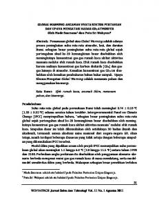
Figure 1. Smoothed estimates of A1 (solid line) and Southern Hemisphere temperature (dotted line).

(i.e., AR(p) model). The accuracy of this approximation (which ignores the potential moving average part of the process) depends on how close the MA part of the true process is to the boundary of the invertibility region. That is, how close the roots of the MA polynomial are to the unit circle (Harvey, 1993). Harvey (1993) argues that the roots of the MA polynomial are likely to be near the unit circle when the true process is I(2). For example, in the local linear trend model (Equations (1) through (3)), which corresponds to a reduced form ARIMA(0,2,2) model, the variance of the slope disturbance (ζt ) generally is small in relation to the variances of the other two error terms. This means that the MA part of the process is close to non-invertibility. ‘The net result is that distinguishing between I(1) and I(2) processes is likely to be very difficult in practice, with the AR based stochastic trend tests tending to favour I(1) specifications, even when I(2) models are appropriate’ (Harvey, 1993, p. 134). The presence of MA components also affects tests where the null hypothesis is an I(1) stochastic trend, and causes them to reject the null far more often than indicated by the standard distributions (Pantula, 1991). Pantula found that the Dickey–Fuller test performed much better than the Phillips–Perron test, but still

420

DAVID I. STERN AND ROBERT K. KAUFMANN

tended to reject the null too often. This result seems to be replicated in our data, where the Dickey–Fuller test may indicate the presence of a stochastic trend in the temperature series while the Phillips–Perron test clearly rejected the null.

4. Structural Time Series Approach To further investigate the time series properties and dynamics of the hemispheric temperature series we use the structural time series modeling approach promoted by Harvey (1989). Structural time series models cover a wide range of models but all are characterized by estimating trend, cyclical, seasonal, and noise components separately and directly. This approach largely eliminates the difficulties of detecting stochastic trends in noisy series discussed in Section 3. The specific model we use is a vector autoregression with common stochastic trends (see Harvey, 1989, pp. 470–473). The stochastic trends are modeled using the local linear trend model in (1) through (3), while the noise processes (εt ) are modeled using a vector autoregression – i.e., current values of the error in the equation for dependent variable i (εit ) are a linear function of its own past values and of the past errors in the equations for the other dependent variables. This approach specifies the null hypothesis such that each series is stationary with a Gaussian error. A large number of alternative hypotheses can be entertained including deterministic trends and I(1) or I(2) stochastic trends in some or all of the series. The method also can be used to estimate cointegrating vectors. For concreteness, we describe the bivariate model we actually use rather than the general case. Using the terminology of state-space models, the measurement equations (equivalent to conventional regression equations but containing state variables that are not observed directly) are: St = A1t +

+ W1t

Nt = θA1t + A2t + W2t ,

(11) (12)

where S and N are the Southern and Northern Hemisphere temperature series. A1 and A2 are nonstationary state variables – the signal – and W is a vector of two are stationary unobserved noise processes, which represent the short-run dynamics of the model. A1 is a possibly common stochastic trend, θ is an estimated fixed parameter. The exclusion of A2 from the first equation is a necessary identifiability condition. The ordering of the dependent variables is essentially arbitrary – regardless of the ordering, the ‘true trends’ can be recovered using a ‘factor rotation’ (see for example Harman, 1976). Nevertheless, the specification of Equations (11) and (12) may have a direct interpretation. The temperature signal associated with greenhouse gases and solar irradiance, which are relatively similar across the northern and southern hemispheres, may be represented by the shared trend A1 . A2 which appears only in the

A STRUCTURAL TIME SERIES ANALYSIS

421

northern hemisphere (12), may represent anthropogenic sources of tropospheric sulfates, which are emitted largely in the northern hemisphere, where they have their greatest effect (Kiehl and Briegleb, 1993). A shared stochastic trend is not imposed on the model – the hypothesis that temperatures in the northern and southern hemisphere share a stochastic trend can be falsified. If the temperature data do not share a stochastic trend, θ will be zero. Sharing of a stochastic trend implies that the dependent variables are cointegrated. A variety of different forms of cointegration are possible with the form depending on the nature of the estimated trends. If the trend A1 is shared and is I(2) and A2 is deterministic, the variables are CI(2,2) i.e., the cointegration relation completely eliminates the I(2) stochastic trend. If A2 is I(1), the variables are CI(2,1) cointegrated – the cointegration relation converts the I(2) trend to an I(1) residual. The stochastic trends are modeled by the following transition equations: Ait +1 = Ait + λit + ηit λit +1 = λit + υit

i = 1, 2

i = 1, 2 ,

(13) (14)

where υi and ηi are white noise processes. The relevant hypotheses are presented in subsection 2.1 above in relation to Equations (2) and (3). A second necessary identifiability condition is that the covariance matrix of (A, λ) is diagonal (Harvey, 1989). The noise processes are modeled as a stationary vector autoregression: W1t +1 =

p−1 X

8j 11 W1t −j +

g=0

W2t +1 =

p−1 X g=0

p−1 X

8j 12 W2t −j + ε1t

(15)

8j 22 W2t −j + E21 ε1t + ε2t ,

(16)

g=0

8j 21 W1t −j +

p−1 X g=0

where the εi are white noise processes, p is the optimal lag length, and the 8j are matrices of coefficients. The model described by Equations (11) through (16) is estimated using the Kalman filter. Under the assumption that the εi random errors are Gaussian, the Kalman filter is used to compute the likelihood function using the prediction error decomposition (Schweppe, 1965; Harvey, 1989). The fixed parameters: 8, θ, and the square roots of the covariance matrices of ε, η, and υ designated E, H , and U ; are estimated by maximizing this likelihood function using the Davidon, Fletcher, Powell algorithm (Fletcher and Powell, 1963; Hamilton, 1994). Then the Kalman filter is used to predict the optimal values of At +1 and Wt +1 using the data in the sample up to period t. A second algorithm, the Kalman smoother, then calculates the optimal values of the state variables given the data in the entire sample. The initial conditions for the non-stationary variables, A and λ, are handled using the diffuse Kalman filter algorithm of de Jong (1988, 1991a,b).

422

DAVID I. STERN AND ROBERT K. KAUFMANN

This algorithm sets Ai0 and λi0 equal to zero with variance equal to the variances of their respective error processes. The Kalman smoother computes the actual optimal mean and variance of Ai0 and λi0 - these can take any value. The variance of ε1 was concentrated out of the likelihood function – i.e., E11 is set to one. 5. Results of Analysis of Observed Data 5.1.

SELECTION OF LAG LENGTH

An array of test statistics is used to select the optimal lag length, p for Equations (15) and (16) (Table II). The longest lag length considered is 5. The likelihood ratio statistics, which are distributed asymptotically as chi-square with 4(5-p) degrees of freedom, indicate that restrictions that reduce the lag length to 1 or 2 lags relative to 5 lags are rejected at the 10% level. Restrictions that reduce the lag length to 3 or 4 are not rejected. The Akaike Information Criterion (AIC) indicates that 3 lags is optimal while the Schwartz Bayesian Criterion (see Enders, 1995) indicates that one lag is the optimal lag length. This latter criterion usually indicates a shorter lag then the AIC. The Durbin–Watson statistic tests for first order serial correlation in the residuals and the Q statistic is a test of all autocorrelation coefficients up to the lag specified. The residuals in all models are not found to be serially correlated, though the residuals for models with lags of 3 to 5 are closer to white noise than those for models with lag lengths of 1 and 2. These results are consistent with the Ljung–Box Multivariate Autocorrelation Test (Ljung and Box, 1978). This generalization of the Q statistic is approximately distributed as χ 2 with n2 (T /4) degrees of freedom, where n is the number of measurement equations. The statistic is calculated over autocorrelations up to T /4 lags. Though none of the test statistics is significant at normal levels of significance, there is a big jump in the significance level between 2 and 3 lags. We choose 3 lags as this is the optimal lag according to both likelihood ratio and AIC criteria and appears to have better residual properties than the 1 and 2 lag models. 5.2.

ESTIMATES FOR THE OPTIMAL MODEL

Parameter estimates for the 3 lag model are presented in Table III. The standard errors are calculated using the Berndt et al. (1974) method for computing the parameter covariance matrix. It is not possible to apply the Berndt et al. algorithm directly to the diffuse Kalman filter. We apply the algorithm to a non-diffuse Kalman filter initiated with the initial state vector and state vector covariance estimated by the smoothing algorithm applied to the diffuse Kalman filter described above. Evidence from a direct likelihood ratio test on U11 using the diffuse Kalman filter model indicates that the estimated standard errors are fairly accurate. Factors that may cause parameter uncertainty not reflected in the estimated covariance matrix include the preliminary specification search described above, and the moderate

423

A STRUCTURAL TIME SERIES ANALYSIS

TABLE II Selection of lag length – observed data # of lags

Log likelihood

Likelihood ratio test

AIC

SBC

Durbin– Watson

Q(35)

Ljung–Box multivariate autocorrelation test

1

610.7901

31.61672 (0.011)

–1199.58

–1167.14

1.7293 1.7824

34.3559 (0.499) 28.1243 (0.789)

167.0809 (0.135)

2

616.7613

19.67432 (0.074)

–1203.52

–1159.29

2.4134 2.0716

38.6298 (0.309) 39.5637 (0.273)

165.6472 (0.105)

3

624.4733

4.25026 (0.834)

–1210.95

–1154.92

2.1023 2.1820

24.7186 (0.902) 32.6332 (0.583)

131.4171 (0.595)

4

625.5760

2.04498 (0.727)

–1205.15

–1137.33

2.1160 2.1545

24.2980 (0.912) 23.4163 (0.932)

119.4982 (0.842)

5

626.5984

–1199.20

–1119.58

2.0944 2.0463

26.2477 (0.857) 23.7483 (0.925)

117.6875 (0.809)

–

Likelihood ratio test is for restriction relative to five lags – significance level in parentheses. For Durbin–Watson and Q statistics, the first number is for the Southern Hemisphere equation and the second statistic is for the Northern Hemisphere equation. For the Q statistic the figure in parentheses is the level of significance.

length of the time series for establishing whether the process is non-stationary or in fact mean-reverting. The parameters of greatest interest are H , U , and θ. Both H11 and U11 are nonzero which means that A1 probably is an I(2) trend. The distribution of the t-test for U11 is non-standard such that the correct critical values for the x% significance level are those for the 2x% significance level in the standard tables (Harvey, 1989; Chernoff, 1954). Therefore, in a one-sided t-test U11 is significant at approximately 15%. In other words, given this sample there is an 85% probability that A1 is I(2) and a 15% probability that A1 is I(1). As discussed below, this trend may represent the aggregate effects of trace gases, changes in

424

DAVID I. STERN AND ROBERT K. KAUFMANN

TABLE III Parameter estimates for optimal model – observed data Parameter

Estimate

Standard error

t-statistic

Parameter

Estimate

Standard error

t-statistic

θ 8111 8112 8121 8122 8211 8212 8221 8222 8311

1.64821 0.49045 –0.06653 0.34006 0.06296 –0.11735 –0.13863 –0.37439 0.00463 0.30638

0.08987 0.12565 0.09675 0.15936 0.11713 0.12267 0.09717 0.13741 0.12118 0.11663

18.33900 3.90329 –0.68765 2.13395 0.53751 –0.95664 –1.42667 –2.72465 0.03821 2.62702

8312 8321 8333 E21 E22 H11 H22 U 11 U 22 σε21

–0.13401 0.30687 –0.37682 0.45014 1.08918 0.25698 0.19507 0.00408 0 0.0788

0.09984 0.15677 0.12399 0.12016 0.10173 0.07554 0.08547 0.00789 n.a. 6.99E-04

–1.34227 1.95742 –3.03912 3.74631 10.70665 3.40211 2.28236 0.51679 n.a. 112.7325

solar irradiance, and the net non-stationary feedback of temperature between the two Hemispheres. All these will add I(1) type ‘noise’ to the trend such that it is still fairly difficult to distinguish between I(2) and I(1) specifications. Figure 1 shows the smoothed estimates of A1 compared to the Southern Hemisphere temperature series. H22 is nonzero, but U22 is zero. Therefore, A2 is an I(1) trend and the two temperature series CI(2,1) cointegrate. The estimate of θ is 1.64821; the cointegrating relationship normalized on Northern Hemisphere temperatures is therefore: Nt − 1.64821 St = A2t .

(17)

This implies that the common trend (A1 ) has a 65% greater impact on Northern Hemisphere temperatures then on Southern Hemisphere temperatures. The estimate of (θ − 1) is highly statistically significant (t = 7.22). If this common trend is associated with the radiative forcing due to greenhouse gases and solar irradiance, this difference in climate sensitivity may be generated by differences in land/water ratios between hemispheres and other factors. σ 2 ε1 is the estimate of the variance of ε1 that was concentrated out of the likelihood function. All the error variances are scaled by this variance. The remaining parameters are best summarized in terms of the companion matrix (Hansen and Juselius, 1995). The maximum eigenvalue of this matrix is 0.74365, which indicates that the noise process is indeed stationary.? Most of these parameters are formally significantly different from zero. ? A maximum eigenvalue of 0.9 or greater might be taken as evidence of a unit root in the process. We do not have any statistical information on the precision of the estimated eignevalues. This is merely a heuristic rule.

A STRUCTURAL TIME SERIES ANALYSIS

5.3.

425

ORIGINS OF THE STOCHASTIC TRENDS

To identify the origins of the stochastic trends, we compare the estimated stochastic trends to historical time series for variables that may affect temperature. These variables include radiative forcing due to greenhouse gases, anthropogenic sulfur emissions, and solar irradiance. Though A1 may be related to radiative forcing of greenhouse gases, the two series might not cointegrate to a stationary residual (CI(2,2)) because of the very long lags inherent in the transmission mechanisms between changes in radiative forcing and changes in temperature. Over several decades, the two series might maintain a linear equilibrium relationship. Under these conditions, the two I(2) series would CI(2,1) cointegrate such that their linear combination is an I(1) process, whereas the two series are I(2) individually. A stationary residual might be obtained by regressing the residual on the first differences of the greenhouse gas radiative forcing and other I(1) variables – solar irradiance and sulfur emissions in our case. This is known as polynomial cointegration (Yoo, 1986). CI(2,1) cointegration also implies that there will be cointegration between the first differences of the relevant I(2) series so we also estimate a regression of this type. This system can be written in the so-called ‘triangular representation’ (Phillips, 1991; Stock and Watson, 1993): A1t = α11 + α12 Sunt + α13 SOxt + α14 GHGt + α15 1GHGt + u1t

(18)

A2t = α21 + α22 Sunt + α23 SOxt + α25 1GHGt + u2t

(19)

1Sunt = α31 + u3t

(20)

1SOxt = α41 + u4t

(21)

12 GHGt = α51 + u5t .

(22)

The system has an equation for each of the relevant variables which has a stationary error process uit . All non-temperature variables are measured by their radiative forcing. A maximum likelihood estimator is derived by second differencing (18), first differencing (19) and collecting terms (Phillips, 1991; Kitamura, 1995): A1t = α11 + α12 Sunt −1 + α13 SOxt−1 + α14 (1 + 1)GHGt −1 + + α15 1GHGt −1 + v1t

(23)

A2t = α21 + α22 Sunt −1 + α23 SOxt−1 + α25 1GHGt −1 + v2t .

(24)

The system (20) to (24) is jointly estimated using the seemingly unrelated regression equations method. The results are presented in Table IV. Though equations (23) and (24) do not cointegrate according to the Augmented Dickey–Fuller and Phillips–Ouliaris tests, the KPSS test fails to reject the null hypothesis that the equations do cointegrate. Greenhouse gases and A1 CI(2,1) cointegrate as shown

426

DAVID I. STERN AND ROBERT K. KAUFMANN

TABLE IV Auxiliary regressions: Observed data Model

Triangular representation

Dependent variable

A1

Constant

–0.3270 0.4177 (–30.6042) (102.6431)

A2

First differences regression 1Sun

SOx

0.001726 –0.007231 (0.6215) (–3.9503)

12 GHG

0.0001648 (0.1678)

1A1

0.002595 (2.4305)

Sun

0.4019 (8.5608)

0.1123 (5.8694)

SOx

0.0997 (1.9760)

0.4100 (43.7841)

GHG

0.2845 (10.0800)

1GHG

–1.2068 (–3.8834)

–0.4329 (–3.4462)

Adjusted R 2

0.9378

0.9781

0

0

0

0.0517

Durbin–Watson

0.1702

0.3437

0.9126

1.8388

2.0556

0.9153

Augmented Dickey–Fuller

–3.9120 (–4.20)

–3.9317 (–3.84)

–7.0823 (–2.45)

–8.9811 (–2.45)

–14.1239 (–2.45)

–4.1184 (–3.13)

Phillips–Perron– Ouliaris

–3.3394 (–4.20)

–3.5294 (–3.84)

–6.4378 (–2.45)

–10.5351 (–2.45)

–11.7912 (–2.45)

–6.0619 (–3.13)

0.2239 (0.347)

0.2201 (0.347)

0.0473 (0.347)

0.1194 (0.347)

0.0130 (0.347)

0.1280 (0.347)

KPSS

0.1389 (2.9019)

For regression coefficients figures in parentheses are t-statistics. For cointegration statistics figures in parentheses are critical values for the 10% significance level. Cointegration statistics are based on the primitive model. ADF and PPO tests have null of non-cointegrations. KPSS has null of cointegration. Critical values for ADF and PPO from Phillips and Ouliaris (1990).

by the cointegration test statistics in the first differences regression 1A1 = 0.002595 + 0.1389 1GHG (Table IV). This indicates that the residual in the levels regression would be I(1). If these regressions do cointegrate, then it is unlikely that there could be alternative causes of systematic change in temperature that we have ignored. The evidence above is mixed, depending on which test is used. The KPSS test suggests that (20) to (24) is an adequate explanation of the extracted

A STRUCTURAL TIME SERIES ANALYSIS

427

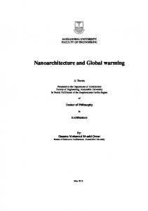
Figure 2. Estimates of A1 from observed data and Hadley Centre model (solid lines) and fitted models for the two data sets (dotted lines). Observed and Hadley data are offset by an arbitrary 0.25 K.

trends, while the other two tests suggest that there may be further significant factors causing temperature change. The coefficient on GHG in (23): 0.2845 indicates that the climate sensitivity in the Southern Hemisphere for doubling CO2 is 1.2422 K. The coefficient on the first difference of greenhouse gas radiative forcing represents medium term adjustment dynamics and doesn’t have a simple interpretation. Solar irradiance has a greater effect per unit of radiative forcing than the greenhouse gases on Southern Hemisphere temperature. Anthropogenic sulfur emissions have a small effect. Feedback between the hemispheres will cause effects in one hemisphere to be transmitted in an attenuated form to the opposite hemisphere. The relationship between A1 and its fitted model is illustrated in Figure 1. The model for A2 (24), which is unique to the northern hemisphere, indicates the major role for sulfur emissions with a lesser role for the differences in the effects of solar irradiance between the two hemispheres. The solar effect is even stronger in this hemisphere than in the southern hemisphere relative to the effect of greenhouse gases. Figure 2 illustrates the fit between trend and model. The long run

428

DAVID I. STERN AND ROBERT K. KAUFMANN

relationship for temperature in the Northern Hemisphere is given by multiplying the coefficients in (23) by θ and adding the coefficients in (24): θA1 + A2t = −0.1213 + 0.7747Sunt + 0.5743SOxt + 0.4689GHG − 2.42201GHGt + θu1t + u2t .

(25)

The climate sensitivity in the Northern Hemisphere for doubling CO2 is 2.0476 K. The global mean climate sensitivity is, therefore, 1.6449 K, which is at the low end of the range estimated by climate models (1.5–4.5 ◦ C).

6. Results of Analysis of Hadley Centre Model Data 6.1.

MOTIVATION

We apply the same structural time series model methodology to the output of the SUL experiment run on the Hadley Centre GCM (Mitchell et al., 1995). This experiment allowed the radiative forcing of the atmosphere to increase at a rate consistent with the change in the CO2 equivalent of all greenhouse gases and anthropogenic sulfur emissions over the 1860–1990 historical period. The simulation increases the concentration of the greenhouse gases and sulfates in the 1991–2099 forecast horizon according to IPCC emission scenarios. The results from this exercise can be used in two ways. First, this data set contains the features thought by climate scientists to be of importance if the global warming hypothesis is true. If we obtain results similar to those generated from the observed data, the probability of a type I error that the null hypothesis of no anthropogenic global warming has been rejected incorrectly is reduced further. Alternatively, the results can be seen as a test of the ability of the Hadley Centre model to reproduce the principal features of the data as decomposed by the structural time series model in the previous section. 6.2.

SELECTION OF LAG LENGTH

We use the same test statistics to select the optimal lag length (Table V). In this case, the AR(1) model for the noise process is clearly optimal. The AIC and SBC are both at a minimum for this specification and the likelihood ratio statistic for this restriction relative to the AR(5) model is insignificant. The auto-correlation statistics all show that this model is adequately specified – none of the test statistics are statistically significant. 6.3.

ESTIMATES FOR THE OPTIMAL MODEL

The results for the AR(1) model are given in Table VI. As in the case of the observed data there are two stochastic trends. Evidence that the A1 trend is I(2)

429

A STRUCTURAL TIME SERIES ANALYSIS

TABLE V Selection of lag length – Hadley Centre model data # of lags

Log likelihood

Likelihood ratio test

AIC

SBC

Durbin– Watson

Q(35)

Ljung–Box multivariate autocorrelation test

0

520.4702

35.3564 (0.0183)

–1026.94

–1006.50

1.5477 2.4927

63.9197 (0.0014) 45.1226 (0.0962)

158.5863 (0.0573)

1

534.2473

7.8022 (0.9545)

–1046.49

–1014.37

1.9784 2.1093

40.8524 (0.1947) 31.0639 (0.6123)

115.1751 (0.8512)

2

535.2439

5.8090 (0.9254)

–1040.49

–996.69

2.0622 2.0206

38.6504 (0.2676) 29.5523 (0.6854)

117.4105 (0.8138)

3

536.4908

3.3152 (0.9130)

–1034.98

–979.50

2.1313 2.0602

30.6221 (0.6340) 27.7238 (0.7678)

111.1010 (0.9065)

4

537.9156

0.4656 (0.9768)

–1029.81

–962.67

2.1352 2.0607

25.0603 (0.8674) 24.9194 (0.8718)

98.1690 (0.9878)

5

538.1484

n.a.

–1022.30

–943.46

2.1314 2.0379

24.5223 (0.8839) 25.1323 (0.8651)

89.5255 (0.9961)

Likelihood ratio test is for restriction relative to five lags – significance level in parentheses. For Durbin Watson and Q statistics, the first number is for the Southern Hemisphere equation and the second statistic is for the Northern Hemisphere equation. For the Q statistic the figure in parentheses is the level of significance.

430

DAVID I. STERN AND ROBERT K. KAUFMANN

TABLE VI Parameter estimates for optimal model – Hadley Centre model data Parameter

Estimate

Standard error

t-statistic

Parameter

Estimate

Standard error

t-statistic

θ 811 821 812 822 E21

1.46630 0.36207 0.10758 –0.09033 0.52580 0.31128

0.16161 0.08197 0.06443 0.10974 0.09319 0.06008

9.07283 4.41720 1.66976 –0.82314 5.64243 5.18141

E22 H11 H22 U11 U22 σ 2 ε1

0.68993 0 0 0.00632 0 0.02486

0.05030 n.a. n.a. 0.00321 n.a. 0.0223

13.71679 n.a. n.a. 1.96580 n.a. 10.83408

is stronger than in the results generated from the historical data. The parameter U11 is significant at approximately 1.25%. As H11 is zero the trend is a lot smoother than the trend estimated from the observed data (Figure 3). The second trend A2 is a deterministic linear trend rather than I(1). The estimate of θ is 1.4663, which indicates a smaller hemispheric difference in climate sensitivities than in the observed data model, though we cannot test whether there is a statistically significant difference between the two parameters. These differences in the time series properties of the stochastic trends are mainly due to differences between the observed and modeled northern hemisphere temperatures. The observed and modeled southern hemisphere temperatures are very similar. The mean first difference for the observed southern hemisphere temperatures is 0.0045 K i.e., a 0.45 K per century increase in temperature. The mean first difference for the modeled southern hemisphere temperatures is 0.0043 K. However, for the northern hemisphere the respective means are 0.0066 K and – 7.4E-06 K. The initial temperature in 1860 is particularly high – it is the second highest in the sample and almost exactly equal to that in 1995. Only 1990 has a higher modeled temperature. The smoothness of A1 and the similarity between hemispheres may also be due to the smoothed greenhouse gas and sulfate emission data used by Mitchell et al. (1995). Our greenhouse gas data has not been smoothed. In the earlier years, our data uses cubic spline functions to interpolate the observations of the individual greenhouse gases, but there is no secondary smoothing. Our sulfur data uses individual estimates for each year, while the data used by Mitchell et al. (1995) was based on interpolation between decadal estimates. 6.4.

ORIGINS OF THE STOCHASTIC TRENDS

We modify the analysis to take into account the fact that the Hadley model does not have a solar input and that our estimates show that the difference between the

A STRUCTURAL TIME SERIES ANALYSIS

431

Figure 3. Smoothed estimates of A2 in the observed data (solid line) and fitted model (dotted line).

stochastic trends in the two hemispheres is deterministic. We use Equation (18) with the solar variable dropped and estimate a version of (25) also without the solar variable. These two equations are jointly estimated with (21) and (22). We use the original forcing series used in the GCM simulation. The results appear in Table VII. Parameter estimates for the levels variables are similar to those for the observed data model with two exceptions. SOx has a significant negative effect in the Southern Hemisphere and 1GHG has a positive effect in the Northern Hemisphere. The fit (Adjusted R 2 = 0.9121) in the Northern Hemisphere is poorer than in the Southern Hemisphere. As for cointegration, only the KPSS statistic shows strong evidence of cointegration for the first equation. The northern hemisphere equation shows greater evidence of cointegration. The first difference model cointegrates rather poorly. We conclude that the results based on the Hadley Centre GCM output are similar to those from the observed data. The difference between temperatures in the two hemispheres is more linear in the Hadley Centre model than in the observed data. This is primarily due to differences between the model and data in the Northern Hemisphere. The model output is very similar to the data in the southern hemisphere. The input data series are smoothed approximations to the observed data.

432

DAVID I. STERN AND ROBERT K. KAUFMANN

TABLE VII Auxiliary regressions Hadley model Model

Triangular representation

Dependent variable

A1

θA1 + A2

1SOx

Constant

–0.2784 (–204.0628)

–0.1362 (–16.7086)

–0.005072 (–7.5240)

SOx

–0.3377 (–38.5182)

0.6725 (12.8766)

GHG

0.2381 (51.1439)

0.2622 (9.4541)

1GHG

–0.4917 (–4.2180)

7.5329 (10.8482)

Adjusted R 2

0.9991

0.9121

0

0

0.8621

Durbin–Watson

0.2259

0.2296

2.2379

1.7230

0.1034

Augmented Dickey–Fuller

–2.8221 (–3.84)

–3.7146 (–3.84)

–1.9304 (–2.45)

–8.1676 (–2.45)

–2.6725 (–3.13)

Phillips–Perron– Ouliaris

–2.7052 (–3.84)

–3.9359 (–3.84)

–12.7950 (–2.45)

–9.7423 (–2.45)

–2.5995 (–3.13)

0.1068 (0.347)

0.3322 (0.347)

KPSS

First differences regression 12 GHG

0.0003518 (2.1936)

1A1

0.0009665 (5.30887)

0.2569 (28.8543)

1.33579 (0.347)

0.38514 (0.347)

0.5674 (0.347)

For regression coefficients figures in parentheses are t-statistics. For cointegration statistics figures in parentheses are critical values for the 10% significance level. Cointegration statistics are based on the primitive model. ADF and PPO tests have null of non-cointegrations. KPSS has null of cointegration. Critical values for ADF and PPO from Phillips and Ouliaris (1990).

This is probably a major cause of the smoother estimated stochastic trends and the poorer cointegration in the regression model fitted to those stochastic trends. Figure 2 illustrates the fit of the model to the estimate of A1 for the Hadley data. The fit is very good in the middle and later parts of the sample but poorer in the early years.

A STRUCTURAL TIME SERIES ANALYSIS

433

7. Conclusions The results of the structural time series model presented in this paper indicate that there may be a global warming signal – an I(2) stochastic trend – present in hemispheric temperature series. Univariate stochastic trend tests have difficulty in detecting this trend due to the low signal to noise ratio of the temperature series. Even so, the relevant estimated parameter is only significant at the 15% level of significance. This result is, therefore, tentative. The difference between the temperature series in the two hemispheres may be due to sulfur emissions in the Northern Hemisphere and the greater climate sensitivity of Northern Hemisphere temperatures. Analysis of output from the Hadley Centre GCM using the structural time series methodology shows a similar pattern to the observed data analysis. The major difference between the GCM model and the historical data is in the modeling of Northern Hemisphere temperatures. This seems to be due to the way the Hadley Centre Model simulates the effect of tropospheric sulfates. This is not so surprising because this was one of the first transient experiments that included the sulfate input. Also the forcing variables used in the Hadley modeled were smoothed, while our input variables are unsmoothed. Smoothing destroys some of the evidence that cointegration analysis aims to uncover. These results reinforce both our own previous work (Kaufmann and Stern, 1997) and other work which suggested these hypotheses (Wigley, 1989). The Hadley model results show that if the climate system works in the way presumed by the model, then the temperature series should contain an I(2) stochastic trend. This means that our search for an I(2) signal in the observed temperature series makes physical sense. While connection of the common stochastic trend in the temperature series to radiative forcing due to greenhouse gases and solar irradiance is tentative, our work shows that such a global warming signal could be present in the temperature series. This is contrary to the interpretation of Woodward and Gray (1993, 1995) that the presence of a stochastic trend in temperature is evidence that the current warming may not continue.

Acknowledgements We thank L. Danny Harvey, Judith Lean, Makiko Sato, and Mark Battle for providing data. John Norton, Roger Perman, and two anonymous referees provided very useful comments.

434

DAVID I. STERN AND ROBERT K. KAUFMANN

Appendix A. Data Sources We have assembled an annual time series data set for the period 1856 to the present for the variables described below. A . 1 . TEMPERATURE

We examine three temperature indicators – global mean annual temperature, and series for the Northern and Southern Hemispheres separately. These data have not been adjusted for ENSO. These data are available from Jones et al. (1994). A . 2 . CARBON DIOXIDE

Data for direct observations for the atmospheric concentration of carbon dioxide are available from the Mauna Loa observatory starting in 1958. Prior to 1958, we used data from the Law Dome DE08 and DE08-2 ice cores (Etheridge et al., 1996). We interpolated the missing years using a natural cubic spline and two years of the Mauna Loa data (Keeling and Whorf, 1994) to provide the endpoint. The data set can be updated in a consistent manner based on annual observations from Mauna Loa. Radiative forcing is calculated using the formula in Kattenberg et al. (1996). A . 3 . METHANE

Indirect observations for the atmospheric concentration of methane are available from the Law Dome ice core (Etheridge et al., 1994). These data are available starting in 1841 and end in 1978. Observations are not available for every year and some years have multiple observations. We use a cubic spline to generate a consistent set of annual observations. From 1968 on we combine these data with the Battle et al. (1996) firn data to obtain a smooth series. The values in the Battle et al. series are scaled down to match the levels in the ice core. 1979–1983 is based on the firn data. 1983 is based on actual observations at Palmer Station (Dlugokencky et al., 1994). 1984–1986 are observations from Cape Grim (Dlugokencky et al., 1994). The remainder of the data – 1987–1995 – are also from Cape Grim but collected by Prinn et al. (1990) in the GAGE/AGAGE network. The latter data were downloaded from CDIAC (Prinn et al., 1997) and are described in Prinn et al. (1990). Accounting for the effects of tropospheric ozone and stratospheric water vapor due to methane (Kattenberg et al., 1996) and the overlap with nitrous oxide, we √ √ calculate that radiative forcing is given by approximately 0.0387 ( Mt − M1860) where M is in ppbv. A . 4 . CFC s

Prather et al. (1987), have generated estimates for years prior to 1978 based on historical emissions and a general model of atmospheric mixing. Direct observations

A STRUCTURAL TIME SERIES ANALYSIS

435

for the atmospheric concentration of CFC-11 and CFC-12 are available starting in 1978 (Cunnold et al., 1994). For CFC-11 we used the data for Adrigole and Mace Head in Ireland. Missing years were filled using the rates of change in the data from the Barbados station. For CFC-12 we used the data from Barbados which more closely match the Prather et al. data for this gas. Including the radiative forcing due to ozone depletion (Kattenberg et al., 1996, Wigley and Raper, 1992) gives the following formulae: CFC-11 0.22y − 0.0552(3y)1.7 CFC-12 0.28z − 0.0552(2z)1.7 , where y and z are in parts per billion. A . 5 . NITROUS OXIDE

Data from 1978 to the present are observations from Cape Grim in the ALE/GAGE/ AGAGE network (Prinn et al., 1990; Prinn et al., 1997). Pre-1978 is based on data from the H15 Antarctica ice core reported in Machida et al. (1995) and the Battle et al. (1996) firn data. We discard a number of observations from the Machida et al. (1995) data based on the fit with the Battle et al. (1996) firn data and fitted √ a cubic spline to the remaining data. Radiative forcing is assumed to be 0.1325 ( Nt − √ N1860) where N is in ppbv. The coefficient is reduced from 0.14 to account for the overlap with methane. A . 6 . AEROSOLS

We use estimates of stratospheric aerosols from Sato et al. (1993). The radiative forcing due to these emissions has been estimated by L. D. Harvey (personal communication). We use estimates of anthropogenic emissions of SOx rather than ice core records of tropospheric sulfate aerosol densities. For 1860 to 1990 we use estimates prepared by A.S.L. and Associates (1997). The estimates are updated to 1994 using methods documented in Stern and Kaufmann (1996). Radiative forcing is assumed to be –0.3 (St /S1990)−0.8 ln(1+St /42)/ ln(1+S1990 /42) where S is in megatonnes (Kattenberg et al., 1996; Wigley and Raper, 1992). The emissions are modified to account for the increase in stack heights over time (Wigley and Raper, 1992). A . 7 . SOLAR ACTIVITY

The effect of solar activity on the planetary heat balance is represented using the index of solar irradiance assembled by Lean et al. (1995). Radiative forcing is linear in irradiance and equal to 0.175 times the change in irradiance (Shine et al., 1991).

436

DAVID I. STERN AND ROBERT K. KAUFMANN

References Akaike, H.: 1973, ‘Information Theory and an Extension of the Maximum Likelihood Principle’, in Petrov, B. N. and Csaki, F. (eds.), 2nd International Symposium on Information Theory, Akademini Kiado, Budapest, pp. 267–281. Andrews, D. W. K.: 1991, ‘Heteroskedasticity and Autocorrelation Consistent Covariance Matrix Estimation’, Econometrica 59, 817–858. A.S.L. and Associates: 1997, Sulfur Emissions by Country and Year, Report No. DE96014790, U.S. Department of Energy, Washington D.C. Battle, M., Bender, M., Sowers, T., Tans, P. P., Butler, J. H., Elkins, J. W., Ellis, J. T., Conway, T., Zhang, N., Lang, P., and Clarke, A. D.: 1996, ‘Atmospheric Gas Concentrations over the Past Century Measured in Air from Firn at the South Pole’, Nature 383, 231–235. Berndt, E., Hall, B., Hall, R. E., and Hausman, J. A.: 1974, ‘Estimation and Inference in Non-Linear Structural Models’, Ann. Econ. Soc. Measure. 55, 653–665. Chernoff, H.: 1954, ‘On the Distribution of the Likelihood Ratio’, Ann. Math. Stat. 25, 573–578. Cunnold, D., Fraser, P., Weiss, R., Prinn, R., Simmonds, P., Miller, B., Alyea, F., and Crawford, A.: 1994, ‘Global Trends and Annual Releases of CCl3F and CCl2F2 Estimated from ALE/GAGE and Other Measurements from July 1978 to June 1991’, J. Geophys. Res. 99 (D1), 1107–1126. De Jong, P.: 1988, ‘The Likelihood for a State Space Model’, Biometrika 75, 165–169. De Jong, P.: 1991a, ‘Stable Algorithms for the State Space Model’, J. Time Ser. Anal. 12 (2), 143–157. De Jong, P.: 1991b, ‘The Diffuse Kalman Filter’, Ann. Stat. 19, 1073–1083. Dickey, D. A. and Fuller, W. A.: 1979, ‘Distribution of the Estimators for Autoregressive Time Series with a Unit Root’, J. Amer. Stat. Assoc. 74, 427–431. Dickey, D. A. and Fuller, W. A.: 1981, ‘Likelihood Ratio Statistics for Autoregressive Processes’, Econometrica 49, 1057–1072. Dlugokenchy, E. J., Lang, P. M., Masarie, K. A., and Steele, L. P.: 1994, ‘Global CH4 Record from the NOAA/CMDL Air Sampling Network’, in Boden, T. A., Kaiser, D. P., Sepanski, R. J., and Stoss, F. S. (eds.), Trends ’93: A Compendium of Data on Global Change, ORNL/CDIAC-65, Carbon Dioxide Information Analysis Center, Oak Ridge National Laboratory, Oak Ridge, TN, pp. 262–266. Enders, W.: 1995, Applied Econometric Time Series, John Wiley, New York. Engle, R. E. and Granger, C. W. J.: 1987, ‘Cointegration and Error-Correction: Representation, Estimation, and Testing’, Econometrica 55, 251–276. Etheridge, D. M., Pearman, G. I., and Fraser, P. J.: 1994, ‘Historical CH4 Record from the “DE08” Ice Core at Law Dome’, in Boden, T. A., Kaiser, D. P., Sepanski, R. J., and Stoss, F. S. (eds.), Trends ’93: A Compendium of Data on Global Change, ORNL/CDIAC-65, Carbon Dioxide Information Analysis Center, Oak Ridge National Laboratory, Oak Ridge, TN, pp. 256–260. Etheridge, D. M., Steele, L. P., Langenfelds, R. L., Francey, R. J., Barnola, J.-M., and Morgan, V. I.: 1996, ‘Natural and Anthropogenic Changes in Atmospheric CO2 over the Last 1000 Years from Air in Antarctic Ice and Firn’, J. Geophys. Res. 101, 4115–4128. Fletcher, R. and Powell, M. J. D.: 1963, ‘A Rapidly Convergent Descent Method for Minimization’, Computer J. 6, 163–168. Folland, C. K., Karl, T. R., Nicholls, N., Nyenzi, B. S., Parker, D. E., and Vinnikov, K. Y.: 1992, ‘Observed Climate Variability and Change’, in Houghton, J. T., Callander, B. A., and Varney, S. K. (eds.), Climate Change 1992: The Supplementary Report to the IPCC Scientific Assessment, Cambridge University Press, Cambridge, pp. 139–170. Granger C. W. J. and Newbold, P.: 1974, ‘Spurious Regressions in Econometrics’, J. Econometrics 35, 143–159. Haldrup, N.: 1997, A Review of the Econometric Analysis of I(2) Variables, Working Paper No. 199712, Centre for Non-linear Modelling in Economics, University of Aarhus, Aarhus, Denmark. Hamilton, J. D.: 1994, Time Series Analysis, Princeton University Press, Princeton, NJ.

A STRUCTURAL TIME SERIES ANALYSIS

437

Hansen, H. and Juselius, K.: 1995, CATS in RATS: Cointegration Analysis of Time Series, Estima, Evanston IL. Harman, H. H.: 1976, Modern Factor Analysis, University of Chicago Press, Chicago, IL. Harvey, A. C.: 1989, Forecasting, Structural Time Series Models, and the Kalman Filter, Cambridge University Press, Cambridge. Harvey, A. C.: 1993, Time Series Models, 2nd edn., Harvester Wheatsheaf, London. Johansen, S.: 1988, ‘Statistical Analysis of Cointegration Vectors’, J. Econ. Dyn. Control 12, 231– 254. Jones, P. D., Wigley, T. M. L., and Biffa, K. R.: 1994, ‘Global and Hemispheric Temperature Anomalies – Land and Marine Instrumental Records’, in Boden, T. A., Kaiser, D. P., Sepanski, R. J., and Stoss, F. S. (eds.), Trends ’93: A Compendium of Data on Global Change, ORNL/CDIAC65, Carbon Dioxide Information Analysis Center, Oak Ridge National Laboratory, Oak Ridge, TN, pp. 603–608. Kattenberg, A., Giorgi, F., Grassl, H., Meehl, G. A., Mitchell, J. F. B., Stouffer, R. J., Tokioka, T., Weaver, A. J., and Wigley, T. M. L.: 1996, ‘Climate Models – Projections of Future Climate’, in Houghton, J. T., Meira Filho, L. G., Callander, B. A., Harris, N., Kattenberg, A., and Maskell, K. (eds.), Climate Change 1995: The Science of Climate Change, Cambridge University Press, Cambridge, pp. 285–357. Kaufmann, R. K. and Stern, D. I.: 1997, ‘Evidence for Human Influence on Climate from Hemispheric Temperature Relations’, Nature 388, 39–44. Keeling, C. D. and Whorf, T. P.: 1994, ‘Atmospheric CO2 Records from Sites in the SIO Air Sampling Network’, in Boden, T. A., Kaiser, D. P., Sepanski, R. J., Stoss, F. S. (eds.) Trends ’93: A Compendium of Data on Global Change, ORNL/CDIAC-65, Carbon Dioxide Information Analysis Center, Oak Ridge National Laboratory, Oak Ridge, TN, pp. 16–26. Kiehl, J. T. and Briegleb, B. P.: 1993, ‘The Relative Roles of Sulfate Aerosols and Greenhouse Gases in Climate Forcing’, Science 260, 311–314. Kim, K. and Schmidt, P.: 1990, ‘Some Evidence on the Accuracy of Phillips–Perron Tests Using Alternative Estimates of Nuisance Parameters’, Econ. Lett. 34, 345–350. Kitamura, Y.: 1995, ‘Estimation of Cointegrated Systems with I(2) Processes’, Econometric Theory 11, 1–24. Kuo, C., Lindberg, C., and Thomson D. J.: 1990, ‘Coherence Established between Atmospheric Carbon Dioxide and Global Temperature’, Nature 343, 709–714. Kwiatowski, D., Phillips, P. C. B., Schmidt, P., and Shin, Y.: 1992, ‘Testing the Null Hypothesis of Stationarity against the Alternative of a Unit Root: How Sure Are We that Economic Time Series Have a Unit Root’, J. Econometrics 54, 159–178. Lean, J., Beer, J., and Bradley, R.: 1995, ‘Reconstruction of Solar Irradiance since 1610: Implications for Climate Change’, Geophys. Res. Lett. 22, 3195–3198. Ljung, G. M. and Box, G. E. P.: 1978, ‘On a Measure of Lack of Fit in Time Series Models’, Biometrika 65, 297–303. Machida, T., Nakazawa, T., Fujii, Y., Aoki, S., and Watanabe, O.: 1995, ‘Increase in the Atmospheric Nitrous Oxide Concentration during the Last 250 Years’, Geophys. Res. Lett. 22, 2921–2924. Mitchell, J. F. B., Johns, T. C., Gregory, J. M., and Tett, S. F. B.: 1995, Climate Response to Increasing Levels of Greenhouse Gases and Sulfate Aerosols, Nature 376, 501–504. Newey, W. K. and West, K. D.: 1987: ‘A Simple Positive Semi-Definite Heteroskedasticity and Autocorrelation Consistent Covariance Matrix’, Econometrica 55, 1029–1054. Pantula, S.: 1991, ‘Asymptotic Distributions of Unit-Root Tests when the Process is Nearly Stationary’, J. Busin. Econ. Stat. 9, 63–71. Phillips, P. C. B.: 1991, ‘Optimal Inference in Cointegrated Systems’, Econometrica 59, 283–306. Phillips, P. C. B. and Ouliaris, S.: 1990, ‘Asymptotic Properties of Residual Based Test for Cointegration’, Econometrica 58, 190. Phillips, P. C. B. and Perron, P.: 1988, ‘Testing for a Unit Root in Time Series Regression’, Biometrika 75, 335–346.

438

DAVID I. STERN AND ROBERT K. KAUFMANN

Prather, M., McElroy, M., Wofsy, S., Russel, G., and Rind, D.: 1987, ‘Chemistry of the Global Troposphere: Fluorocarbons as Tracers of Air Motion’, J. Geophys. Res. 92D, 6579–6613. Prinn, R. G., Cunnold, D., Fraser, P., Weiss, R., Simmonds, P., Alyea, F., Steele, L. P., and Hartley, D.: 1997, CDIAC World Data Center Dataset No. DB-1001/R3 (anonymous ftp from [email protected]). Prinn, R. G., Cunnold, D., Rasmussen, R., Simmonds, P., Alyea, F., Crawford, A., Fraser, P., and Rosen, R.: 1990, ‘Atmospheric Emissions and Trends of Nitrous Oxide Deduced from Ten Years of ALE/GAGE Data’, J. Geophys. Res. 95, 18369–18385. Richards, G. R.: 1993, ‘Change in Global Temperature: a Statistical Analysis’, J. Climate 6, 546–559. Sato, M., Hansen, J. E., McCormick, M. P., and Pollack, J. B.: 1993, ‘Stratospheric Aerosol Optical Depths, 1850–1990’, J. Geophys. Res. 98, 22987–22994. Schmidt, P. and Phillips, P. C. B.: 1992, ‘LM Tests for a Unit Root in the Presence of Deterministic Trends’, Oxford Bull. Econ. Stat. 54, 257–287. Schönwiese, C.-D.: 1994, ‘Analysis and Prediction of Global Climate Temperature Change Based on Multiforced Observational Statistics’, Environ. Pollut. 83, 149–154. Schweppe, F.: 1965, ‘Evaluation of Likelihood Functions for Gaussian Signals’, IEEE Trans. Information Theory 11, 61–70. Schwert, G. W.: 1989, ‘Tests for Unit Roots: a Monte Carlo Investigation’, J. Busin. Econ. Stat. 7, 147–159. Shine, K. P. R. G., Derwent, D. J., Wuebbles, D. J., and Mocrette, J. J.: 1991, ‘Radiative Forcing of Climate’, in Houghton, J. T., Jenkins, G. J., and Ephramus, J. J. (eds.), Climate Change: The IPCC Scientific Assessment, Cambridge University Press, Cambridge, pp. 47–68. Stern, D. I. and Kaufmann, R. K.: 1996, Estimates of Global Anthropogenic Sulfate Emissions 1860–1993, CEES Working Papers 9601, Center for Energy and Environmental Studies, Boston University (available on WWW at: http://cres.anu.edu.au/ dstern/mirror.html). Stern, D. I. and Kaufmann, R. K: 1999, ‘Econometric Analysis of Global Climate Change’, Environ. Model. Software 14, 597–605. Stock, J. H. and Watson, M. W.: 1993, ‘A Simple Estimator of the Cointegrating Vectors in Higher Order Integrated Systems’, Econometrica 61, 783–820. Thomson, D. J.: 1995, ‘The Seasons, Global Temperature, and Precession’, Science 268, 59–68. Thomson, D. J.: 1997, ‘Dependence of Global Temperatures on Atmospheric CO2 and Solar Irradiance’, Proc. Natl. Acad. Sci. 94, 8370–8377. Tol, R. S. J.: 1994, ‘Greenhouse Statistics – Time Series Analysis: Part II’, Theor. Appl. Climatol. 49, 91–102. Tol, R. S. J. and de Vos, A. F.: 1993, ‘Greenhouse Statistics – Time Series Analysis’, Theor. Appl. Climatol. 48, 63–74. Tol, R. S. J. and de Vos, A. F.: 1998, ‘A Bayesian Statistical Analysis of the Enhanced Greenhouse Effect’, Clim. Change 38, 87–112. Wigley, T. M. L.: 1989, ‘Possible Climate Change Due to SO2 -Derived Cloud Condensation Nuclei’, Nature 339, 356–367. Wigley, T. M. L. and Raper, S. C. B.: 1992, ‘Implications for Climate and Sea Level of Revised IPCC Emissions Scenarios’, Nature 357, 293–300. Wigley, T. M. L., Smith, R. L., and Santer, B. D.: 1998, ‘Anthropogenic Influence on the Autocorrelation Structure of Hemispheric-Mean Temperatures’, Science 282, 1676–1679. Woodward, W. A. and Gray, H. L.: 1993, ‘Global Warming and the Problem of Testing for Trend in Time Series Data’, J. Climate 6, 953–962. Woodward, W. A. and Gray, H. L.: 1995, ‘Selecting a Model for Detecting the Presence of a Trend’, J. Climate 8, 1929–1937. Yoo, B. S.: 1986, Multi-Cointegrated Time Series and a Generalized Error-Correction Model, University of California at San Diego Department of Economics Discussion Paper. (Received 4 December 1997; in revised form 4 January 2000)