Detecting Changes In Non-Isotropic Images - Mathematics and Statistics

Detecting Changes In Non-Isotropic Images K.J. Worsley1∗, M. Andermann1 , T. Koulis1 , D. MacDonald,2 and A.C. Evans2 August 4, 1999

1

2

Department of Mathematics and Statistics, Montreal Neurological Institute, McGill University, Montreal, Qu´ebec, Canada

3

3

Abstract: If the noise component of image data is non-isotropic, that is, if it has nonconstant smoothness or effective point spread function in every direction, then theoretical results for the P-value of local maxima and the size of supra-threshold clusters of a statistical parametric map (SPM) based on random field theory are not valid. This assumption is reasonable for PET or smoothed fMRI data, but not if this data is projected onto an unfolded, inflated or flattened 2D cortical surface. Anatomical data such as structure masks, surface displacements and deformation vectors are also highly non-isotropic. The solution proposed in this paper is to suppose that the image can be warped or flattened (in a statistical sense) into a space where the data is isotropic. The subsequent corrected P-values do not depend on finding this warping – it is only sufficient to know that such a warping exists. Key words: SPM, random fields. 3

3

∗

Correspondence to: K.J. Worsley, Department of Mathematics and Statistics, McGill University, 805 Sherbrooke St. West, Montreal, Qu´ebec, Canada H3A 2K6. E-mail: [email protected], Web: http://www.math.mcgill.ca/∼keith.

1

¦ Non-Isotropic Images ¦

1

2

INTRODUCTION

The theoretical results for P-values of local maxima and size of supra-threshold clusters of a statistical parametric map (SPM) are not valid if the noise component of the image data is non-isotropic (Worsley et al., 1996). One of the conditions for isotropy or ‘flatness’ (in the statistical sense) is that the FWHM should be the same in all directions and across all voxels in the image. This assumption is reasonable for PET data or smoothed fMRI data, but not for two new types of image data. The first is PET or fMRI data projected onto an unfolded, inflated or flattened 2D cortical surface (Drury et al., 1998; Fischl et al., 1999), where the different amounts of stretching of the surface alter the original constant FWHM, making it non-isotropic. The second is anatomical data such as 3D binary masks of a structure (Zijdenbos et al., 1998), 2D surface displacements (MacDonald et al., 1998), and 3D vector deformations required to warp the structure to an atlas standard (Collins et al., 1998; Thompson et al., 1999). In all these cases, the smoothness of the images varies considerably from region to region, so they too are not isotropic. The purpose of this paper is to present a simple method for overcoming these problems so that random field theory can be applied to most non-isotropic images.

2

METHODS

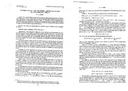
The first step is to transform the data to a triangular (2D) or tetrahedral (3D) lattice. Pixels on a square lattice can be easily transformed by subdividing the squares (of 4 adjacent pixels) into 2 triangles. Voxels on a cubical lattice can be transformed by subdividing each cube of 8 adjacent voxels into 5 tetrahedra as shown in Figure 1 (four round the sides, and one inside). Note that no new vertices (voxels) are created, only their connectivity is altered. Some data, particularly data on cortical surfaces, is already triangulated, so this step is unnecessary.

Figure 1: Voxels (balls) on a cubical lattice can be subdivided into 5 tetrahedra per cube in an alternating checkerboard arrangement.

¦ Non-Isotropic Images ¦

3

The second step is to estimate the effective FWHM (eF W HM ) along each edge of the lattice, defined as the FWHM of a Gaussian kernel that would produce the same local smoothness of the noise component of the observed images. This is based on the normalized residuals from fitting a linear model at each voxel. Label the two voxels at either end of an edge by 1 and 2. We now fit a linear model to data from n images at each voxel by least squares. For image i, let ri1 denote the scalar residual (observed - fitted) at voxel 1, and let ri2 denote the scalar residual at voxel 2, i = 1, . . . , n. The normalized residuals at the ends are rij uij = qPn , i = 1, . . . , n, j = 1, 2. 2 i=1 rij We first estimate the roughness of the noise, defined as the standard deviation of the derivative of the noise divided by the standard deviation of the noise itself. First let v u n uX ∆u = t (ui1 − ui2 )2 . i=1

Then an unbiased estimator of the roughness is λ = ∆u/∆x where ∆x is the length of the edge (Worsley, 1999). For multivariate data, such as 3component vector deformations, the above calculations can be applied separately to each component, then pooled by taking the root mean square of λ across components. The effective FWHM along the edge is then q

eF W HM =

4 loge 2 /λ.

If the image is isotropic or ‘flat’ then the eF W HM should be constant; departures from this indicate non-isotropy. A first attempt at correction is to warp the coordinates of the voxels so that the eF W HM is approximately constant, or equivalently, λ ≈ 1. If the new edge length is ∆˜ x, then this implies that ∆˜ x ≈ ∆u. This is equivalent to a local multidimensional scaling that makes the new edge length ∆˜ x proportional to the old edge length ∆x divided by the eF W HM , which means that edges with low eF W HM are stretched and those with high eF W HM are shrunk (relative to the average). This was achieved by minimising S=

X

(∆˜ x2 − ∆u2 )2

edges

for each point separately, holding all others fixed, then iterating till convergence. By approximating ∆˜ x as a linear function of the warp (ignoring the quadratic term), there is a simple matrix expression for the optimal warp at each iteration. A similar method is covariant regularization (Thompson et al., 1998). Here the data is not warped, but is left in its original configuration. Instead, a new curvilinear mesh is induced in the space of the data, so that any particular tensor (here it would be the smoothness) becomes isotropic in the new coordinate system. However the result is in the end the same; a new coordinate system is defined that makes the data isotropic.

¦ Non-Isotropic Images ¦

4

The usual random field theory for P-values of local maxima and cluster sizes can then be applied to the q resulting isotropic or ‘flattened’ images with constant roughness equal to 1, or FWHM = 4 loge 2. For large search regions, the P-value of local maxima of a SPM T in D dimensions is then well approximated by P(max T ≥ t) ≈ Resels ρD (t), where ρD (t) is the D-dimensional EC density function from Worsley et al. (1996), and D

Resels = V (4 loge 2)− 2 , where V is the area (D = 2) or volume (D = 3) of the search region in the flattened image. The P-value of cluster sizes above a threshold can also be evaluated by simply measuring cluster size in the flattened space and applying the usual formulas (Friston et al., 1995; Cao, 1999). Note that an additional correction is required to account for the randomness of the cluster Resels themselves. This will be the subject of a subsequent paper. However the flattening step is not entirely necessary. Inspection of the preceding calculations shows that Resels can be derived directly from the normalised residuals without actually carrying out the flattening. To see this, let u0 , u1 , . . . , uD be the n-vectors of the normalised residuals at each vertex of a triangular (D = 2) or tetrahedral (D = 3) component of the search region. Define the n × D matrix of differences by ∆u = (u1 − u0 , . . . , uD − u0 ). Then the resels of a region or cluster becomes X 1 D 1 |∆u0 ∆u| 2 (4 loge 2)− 2 . Resels = D! components It can be shown that |∆u0 ∆u| does not depend on which vertex is labelled as 0, and that Resels is unbiased, with no adjustment for degrees of freedom (Worsley, 1999). Note also that Resels does not depend on the actual Euclidean coordinates of the vertices (voxels), only the information about how the voxels are connected to form components. How does this compare with current methods for a square or cubical lattice of voxels? At present, most software for the statistical analysis of SPMs uses the following: ¯ ¯

¯1 ¯2

N ¯¯ X ∆u0 ∆u ¯¯ Resels = D! ¯¯components N ¯¯

D

(4 loge 2)− 2 ,

where N is the number of components, which must all be oriented and labelled in the same way. The discrepancy is then due to summing before or after taking the square root of the determinant, but this discrepancy is slight in practice. However for cluster size statistics there can be a very large discrepancy. The reason is simply this: by chance alone, large size clusters will occur in regions where the images are very smooth, and small size clusters will occur in regions where the image is very rough. The distribution of cluster sizes will therefore be considerably biased towards more extreme cluster sizes, resulting in more false positive clusters in smooth regions. Moreover, true positive clusters in rough regions could be overlooked because their sizes are not large enough to exceed the critical size for the whole region. The proposed method will compensate by replacing cluster size by resel size, which is invariant to differences in smoothness.

¦ Non-Isotropic Images ¦

3

5

RESULTS

As a test, the method was applied to detecting local shape differences between the cortex of normal males (n = 83) and females (n = 68) using smoothed 3D binary masks (Zijdenbos et al., 1998), 2D surface normal displacements (MacDonald et al., 1998) and 3D deformation vectors (Collins et al., 1998). In all cases the eF W HM varied considerably from 5mm to 30mm depending on location, so the images were highly non-isotropic. Despite this, the P-values for local maxima were not greatly affected, but the P-values for cluster sizes were very sensitive to non-isotropy. Details will be reported elsewhere.

4

CONCLUSIONS

We have derived a theoretical method for calculating P-values for local maxima and cluster sizes of non-isotropic image data inside a large search region. The only statistical requirement is that there exists a sufficiently high dimensional space in which the image data can be warped to flatness. Knowing the dimension of this space, or the actual warping into it, is not required. Thus the method can be applied simply and efficiently to a very wide range of non-isotropic image data. For small search regions, the entire flattened image is still necessary to find the remaining boundary correction terms for the unified P-value of local maxima, which is accurate for search regions of almost any shape or size (Worsley et al., 1996). Once again the flattening can be avoided by the following trick. We note that the unified P-value formula does not depend on the dimension of the space used to embed the warped image; a higher dimensional space could be used to achieve a more successful flattening. Taking this to the limit, it can be shown that exact flatness can be achieved by warping the data into a space whose dimensionality equals the number of images: the coordinates are just the normalized residuals. Although this cannot be visualized, the resulting boundary corrections to the P-value can be easily calculated from the resels of the component tetrahedra, triangles and edges alone. This will be pursued in a subsequent paper (Worsley, 1999).

REFERENCES Cao, J (1999). The size of the connected components of excursion sets of χ2 , t and F fields. Advances in Applied Probability, in press. Collins DL, Zijdenbos AP, Evans AC (1998). Improved automatic gross cerebral structure segmentation. NeuroImage, 7:S707. Drury HA, Corbetta M, Shulman G, Van Essen DC (1998). Mapping fMRI activation data onto a cortical atlas using surface-based deformation NeuroImage, 7:S728. Fischl B, Sereno MI, Dale AM (1999). Cortical surface-based analysis: II. Inflation, flattening, and a surface-based coordinate system. NeuroImage, 7:S740.

¦ Non-Isotropic Images ¦

6

Friston KJ, Worsley KJ, Frackowiak RSJ, Mazziotta JC, Evans AC (1994). Assessing the significance of focal activations using their spatial extent. Human Brain Mapping, 1:214-220. MacDonald D, Avis D, Evans AC (1998). Automatic segmentation of cortical surfaces from MRI with partial-volume correction. NeuroImage, 7:S703. Thompson PM, Toga AW, (1998). Anatomically driven strategies for high-dimensional brain image warping and pathology detection. In Toga AW (Ed.), Brain Warping (pp. 311-336). New York: Academic Press. Thompson PM, Woods RP, Mega MS, Toga AW, (1999). Mathematical/computational challenges in creating deformable and probabilistic atlases of the human brain, Human Brain Mapping, [to appear, Sept. 1999]. Worsley KJ, Marrett S, Neelin P, Vandal AC, Friston KJ, Evans AC (1996). A unified statistical approach for determining significant signals in images of cerebral activation. Human Brain Mapping, 4:58-73. Worsley KJ (1999). Exceedence probabilities of local maxima of non-isotropic random fields, with an application to shape analysis via surface displacements. (in preparation). Zijdenbos AP, Giedd JN, Blumenthal JD, Paus T, Rapoport JL, Evans AC (1998). Automatic quantitative analysis of 3D brain data sets: application to a pediatric population. NeuroImage, 7:S727.