Detecting Code Clones in Binary Executables∗ Andreas Sæbjørnsen
†
Jeremiah Willcock
Thomas Panas
University of California, Davis
Indiana University
[email protected]
[email protected]
Lawrence Livermore National Laboratory
[email protected] Zhendong Su
Daniel Quinlan Lawrence Livermore National Laboratory
University of California, Davis
[email protected]
[email protected] ABSTRACT
1.
Large software projects contain significant code duplication, mainly due to copying and pasting code. Many techniques have been developed to identify duplicated code to enable applications such as refactoring, detecting bugs, and protecting intellectual property. Because source code is often unavailable, especially for third-party software, finding duplicated code in binaries becomes particularly important. However, existing techniques operate primarily on source code, and no effective tool exists for binaries. In this paper, we describe the first practical clone detection algorithm for binary executables. Our algorithm extends an existing tree similarity framework based on clustering of characteristic vectors of labeled trees with novel techniques to normalize assembly instructions and to accurately and compactly model their structural information. We have implemented our technique and evaluated it on Windows XP system binaries totaling over 50 million assembly instructions. Results show that it is both scalable and precise: it analyzed Windows XP system binaries in a few hours and produced few false positives. We believe our technique is a practical, enabling technology for many applications dealing with binary code.
Code duplication is common and hinders software maintenance, program comprehension, and software quality. Clone detection, the problem of identifying duplicated code, is thus an important problem and has been extensively studied. Many clone detection algorithms exist [6,13,17–19,21], ranging from basic string-based algorithms [6] to more sophisticated algorithms based on program dependency graphs (PDGs) [13, 19]. Most existing clone detection algorithms operate only on source code, but not on binaries. However, the ability to detect binary clones is important because source code is not always available, for example, in the case of commercial off the shelf (COTS) software. One important application of a practical clone detection algorithm for binaries is the discovery of copyright infringements. A closed-source program could, for example, include GPLed source code in violation of its license; binary-level clone detection may be used to find that. Low-level binaries offer additional interesting challenges for clone detection. First, the problem demands better scalability because a single source statement is normally compiled down to many assembly instructions. Second, various choices made by a compiler, such as register and storage allocation, complicate detection. To see this, consider the following IA-32 assembly code:
∗This
research was supported in part by NSF CAREER Grant No. 0546844, NSF CyberTrust Grant No. 0627749, NSF CCF Grant No. 0702622, US Air Force under grant FA9550-07-1-0532, and an LLNL LDRD subcontract. The information presented here does not necessarily reflect the position or the policy of the Government and no official endorsement should be inferred. This work was performed in part under the auspices of the U.S. Department of Energy by Lawrence Livermore National Laboratory under Contract DE-AC52-07NA27344, and funded by the Laboratory Directed Research and Development Program at LLNL under project tracking code 07-ERD-057. (LLNLPROC-406820) † Work performed while this author was at Lawrence Livermore National Laboratory.
INTRODUCTION
mov mov add mov
[0x805b634], 0x0 [0x805b63c], eax esp, 0x10 eax, ebx
where [0x805b634] dereferences memory location 0x805b634 (similarly for [0x805b63c]), and eax, ebx, and esp are registers. If we use the specific memory addresses or register names for clone detection, we will likely to be too specific and miss true clones. On the other hand, if we simply use opcodes (i.e., mnemonics) of the instructions, we will likely to be too general and report false clones. Third, assembly instructions have a fixed, almost flat structure, while source programs can have arbitrarily deep structures. The rich structural information in source code is a key factor allowing source-level clone detectors, such as Deckard [17], to perform well. All these differences require novel techniques for detecting binary clones. In this paper, we present the first practical binary clone detection algorithm. Our algorithm follows a general tree
Permission to make digital or hard copies of all or part of this work for personal or classroom use is granted without fee provided that copies are not made or distributed for profit or commercial advantage and that copies bear this notice and the full citation on the first page. To copy otherwise, to republish, to post on servers or to redistribute to lists, requires prior specific permission and/or a fee. Copyright 200X ACM X-XXXXX-XX-X/XX/XX ...$5.00.
1
Figure 1: Disassembly and clone detection process. similarity framework [17]: instead of performing a quadratic number of pair-wise comparisons of instruction sequences, it models the essential structural information of the instruction sequences with numerical vectors and groups similar vectors to identify clones. We present novel techniques to generate precise and robust vectors for binaries and to compactly represent the vectors for improved scalability. We have implemented our algorithm and evaluated it on Windows XP system binaries with a total of 50 million instructions. The results indicate that our technique is both scalable and precise. All the Windows XP system binaries can be processed routinely in under a few hours, and the detected clones are accurate with few false positives. Roughly 20% of the code appears in at least one clone cluster, which is consistent with results for source code [17,18,21]. We also evaluate the correspondence of source and binary clones on the Linux kernel, demonstrating that the binary clones our tool detects typically are caused by real clones in the source code. To better understand the potential of our technique, we also consider the impact of compiler optimizations on our results (see Section 5). The rest of the paper is structured as follows. We first provide a high-level overview of our algorithm (Section 2). The detailed algorithm is presented in Section 3. Next, we discuss the implementation (Section 4) and evaluation (Section 5) of our algorithm. Finally, we survey related work (Section 6) and conclude (Section 7).
2.
Figure 2: Example intermediate representation of disassembled binary for stride 1 and window size 3. sequence from Section 1. Notice that each assembly instruction consists of a mnemonic (e.g., “mov”) and an operand list (e.g., “esp, 0x10”). Our intermediate representation preserves all binary file information, including instructions, functions, header information, segments, etc. Section 3.1 describes the representation in more detail. Second, the normalization step (cf. Section 3.2) creates a normalized instruction sequence, abstracting away memoryand register-specific information. The following shows the normalized instruction sequence for the example: mov mov add mov
OVERVIEW
Figure 1 shows the flowchart for our clone detection algorithm. This section explains the process with the help of the simple example from Section 1. Detailed technical descriptions of the steps are be given in the corresponding sections shown in the figure. First, we use a disassembler to process all input binaries and create their intermediate representations. For example, Figure 2 shows how we represent the sample instruction
MEM1, MEM2, REG2, REG1,
VAL1 REG1 VAL2 REG3
Third, we perform clone detection on the normalized instruction sequences. We separate the problem into two cases, mostly for efficiency reasons. One case is exact clone detection, where only identical normalized instruction sequences are returned. The other case is inexact clone detection, where certain differences are tolerated. This is a computationally challenging problem. We use feature vectors to approximate structural characteristics of the given assembly instruction sequences and group similar vectors to find clones. See Sections 3.3.2 and 3.3.3 for more details. We now have a set of clone clusters, i.e., instruction sequences of a certain size1 that are considered similar. For inexact clone detection, the similarity threshold is user-defined while that between instruction sequences for exact clone detection is one. For instance, the clone cluster C = {seq1 , seq2 , seq3 } contains three similar instruction sequences, seq1 , seq2 , and seq3 . Two sequences within a clone cluster, say seq1 and
This [5] document was prepared as an account of work sponsored in part by an agency of the United States government. Neither the United States government nor Lawrence Livermore National Security, LLC, nor any of their employees makes any warranty, expressed or implied, or assumes any legal liability or responsibility for the accuracy, completeness, or usefulness of any information, apparatus, product, or process disclosed, or represents that its use would not infringe privately owned rights. Reference herein to any specific commercial product, process, or service by trade name, trademark, manufacturer, or otherwise does not necessarily constitute or imply its endorsement, recommendation, or favoring by the United States government or Lawrence Livermore National Security, LLC. The views and opinions of authors expressed herein do not necessarily state or reflect those of the United States government or Lawrence Livermore National Security, LLC, and shall not be used for advertising or product endorsement purposes.
1
2
This is referred to as the window as shown in Figure 2.
Algorithm 1 Generate code regions. Input: f : Disassembled instructions for a single function Input: w: Window size Input: s: Stride Output: R: The set of code regions 1: R ← ∅ 2: for i = 0 to length(f ) − w step s do 3: thisRegion ← f[i,i+w) 4: R ← R + thisRegion
seq2 , may overlap substantially and should not be considered clones. Removing such spurious clones is conducted by a postprocessing step (Section 3.4). So far in the detection process, we consider only instruction sequences of a certain predefined length, but reporting many small clones is not as useful as reporting a few large ones. So, in the final step, we combine smaller contiguous clones into larger ones. The algorithm for doing this is presented in Section 3.5.
3.
ALGORITHM DESCRIPTION
This section gives a detailed description of our algorithm, structured according to the flowchart in Figure 1.
3.1
regions within a particular function. As the window size and stride are constant for a particular run, this algorithm takes linear time in the number of vectors produced. For a single function F of length l, the number of vectors generated is b(l − w + 1)/sc.
Binary Disassembly
An assembly instruction is a pair of a mnemonic m and a list of operands o. The mnemonic m represents the particular operation that the instruction performs, and is from a finite set M of possible mnemonics. The list of operands is a variable-length, but typically short, sequence of elements from the set O of possible operands. We partition the set O of operands into three categories: memory references (e.g., “[0x805b634]”), register references (e.g., “eax”), and constant values (e.g., “0x10”). We do not use any of the structure of the individual operands other than this categorization, but we do assume the ability to compare two operands for syntactic equality. In the following algorithm descriptions, an instruction is defined as an element of the set M × O∗ , with O partitioned into Omem , Oreg , and Oval . We use the functions mnemonic and operands to access the two parts of an instruction, and zero-based subscripts (of either single elements or intervals) to indicate accesses to elements or contiguous subsequences of a sequence; the ++ operator is used to indicate sequence concatenation, and the + operator is used to add a single element to a set or bag. The function type maps from O to the set OPTYPE = {MEM , REG, VAL} based on the particular category of an operand. The full disassembly of a particular executable or library is defined as a sequence of functions, with each function containing a sequence of instructions. We define clones in terms of code regions, which are simply contiguous subsequences of the instructions of a single function, along with information on the starting address, function, and file of that list of instructions. We ignore that extra information for clone detection, but it is preserved by our algorithms and used by the postprocessing and visualization stages. We assume that algorithms that create and/or transform code regions implicitly process the extra information appropriately. When the distinction is important, the two functions instructions and extraInfo access the two parts of a code region. The actual process of creating the disassembled instructions for a program and grouping them into functions is implementation-specific; our particular implementation is explained in Section 4. We split each function of a binary into code regions using two parameters window and stride. The window is the length of the code region to generate. The starting points of the code regions within a function are separated by the stride; note that code regions can, and almost always will, overlap. For example, with window size 50 and stride 10, the first three code regions contain instructions 0–49, 10–59, and 20–69 respectively. Algorithm 1 is used to compute the code
3.2
Code Region Normalization
As explained in Section 2, the particular operands used in a code region may be specific to that code region, and so some “fuzziness” should be allowed in clones. For example, two regions may be identical except for certain constant values, offsets in memory locations, or particular addresses used as branch targets. In order to account for these differences, we normalize the instructions in a code region using Algorithm 2. This function takes a list of instructions in the hmnemonic, operandsi format and converts them to abstract instructions of the form hmnemonic, abstract operandsi. An abstract operand is a pair of an operand type (either MEM , REG, or VAL from the set OPTYPE ) and a natural number indicating the index of the first occurrence of that particular operand expression within the code region. The operands are numbered separately for each operand type. The normalization produces an abstract code region, which is just a list of abstract instructions. The normalization algorithm takes linear time in the number of instructions in the code region, and is run once on each code region in the program. Algorithm 2 Normalize a code region. Input: r: Input code region Output: r0 : Output abstract code region /* N is a mapping from OPTYPE to the sequence of /* operands of that type seen so far */ 1: N ← ∅ 2: r0 ← hi with extra info extraInfo(r) 3: for all instructions i in r do 4: ops 0 ← hi 5: for all operands o in operands(i) do 6: t ← type(o) 7: if o is an element of N [t] then 8: idx ← zero-based index of o in N [t] 9: else 10: idx ← length(N [t]) 11: N [t] ← N [t] ++ hoi 12: o0 ← ht, idx i 13: ops 0 ← ops 0 ++ ho0 i 0 14: i ← hmnemonic(i), ops 0 i 15: r0 ← r0 ++ hi0 i
3
Algorithm 3 Find exact clone clusters. Input: R: Set of abstract code regions Output: C: Set of clone clusters, each of which is a set of code regions 1: H ← empty hash table mapping from sequences of abstract instructions to sets of code regions 2: for all code regions r in R do 3: add r to H[instructions(r)] 4: C ← {c ∈ values(H) : |c| ≥ 2}
3.3
Algorithm 4 regionToVector: Generate feature vector. Input: r: Abstract code region Output: v: Feature vector 1: b ← an empty bag (multiset) of features from F 2: for all instructions i in instructions(r) do 3: b ← b + mnemonic(i) 4: for all ht, idx i ∈ operands(i) do 5: if idx < k then 6: b ← b + ht, idx i 7: b←b+t 8: ops ← operands(i) 9: if length(ops) ≥ 1 then 10: b ← b + hmnemonic(i), type(ops 0 )i 11: if length(ops) ≥ 2 then 12: b ← b + htype(ops 0 ), type(ops 1 )i 13: v ← bagToVector (b)
Clone Detection
We define two ways to find clones among binaries: exact matching of normalized code regions, and inexact matching of feature vectors representing important aspects of the code regions. Both of these algorithms use linear time and space to find the initial set of clone clusters.
3.3.1
Definitions of Clone Pairs and Clusters
example, each possible instruction mnemonic is a feature, and each combination of the instruction’s mnemonic and the type of the instruction’s first operand is a feature. The features we use are local to each abstract instruction, and can thus be evaluated independently on the instructions in a code region. We count the number of occurrences of each feature within a code region, producing a feature vector for the region. Formally, a feature vector is a vector of natural numbers of length |F |, based on a fixed but arbitrary order of the features in F . We allow feature vectors to be indexed directly by features rather than requiring an explicit mapping from features to vector indices. We count the following features of an abstract instruction or code region; F is the disjoint union of the sets given. These five categories of features were necessary to include in the feature vectors to accurately characterize the code:
Code regions can appear in clone pairs and in clone clusters. A clone pair is an unordered pair of code regions that are “close enough” (by a metric defined later) to be considered to match. We form clone pairs into clone clusters by finding groups of clone pairs that all contain the same normalized instructions. For exact matching, and in practice for inexact matching, the clone pair relation is transitive, and so choosing the neighbors of an arbitrary code region is appropriate. For measuring the accuracy of our clone detection algorithm, we define false positives and false negatives. A clone pair is considered to be a false positive when it is found by the clone detection algorithm and yet the normalized instruction sequences of the two code regions in the pair are not identical. A clone pair is a false negative if it satisfies the definition of a clone pair given above and yet is not found by our algorithm. False positives and false negatives can never appear when using exact matching of normalized instruction sequences (by definition), but our inexact matching algorithm has both types of error. In order to test the accuracy of our algorithm, we test the inexact matching algorithm with a distance of less than one to simulate exact matching on feature vectors, and determine how well those results match the actual exact matching algorithm. Note that two distinct normalized instruction sequences may have exactly the same feature vector, so there can be false positives in a vector-based matching algorithm even when exact matches of vectors are found.
3.3.2
• M , representing the mnemonic of the instruction; • OPTYPE , representing the type of each operand in an instruction; • M × OPTYPE , representing the combination of the mnemonic and the type of the first operand when one is present; • OPTYPE × OPTYPE , representing the types of the first and second operands, in that order, of an instruction with at least two operands; and • OPTYPE × Nk , representing each normalized operand with an index under a chosen limit k.
Exact Clone Detection
Exact matching uses a traditional hash table on the normalized instruction sequences, as shown in Algorithm 3. Although this algorithm produces a set of clone clusters, the corresponding set of clone pairs can be found by converting the partition C into an equivalence relation. Algorithm 3 requires linear time, and produces exactly the correct set of clone clusters (with neither false positives nor false negatives).
3.3.3
As we treat the window size as a constant, and the number of operands in an instruction is at most a small number, we can treat vector generation for a single code region as a constant-time operation. The overall vector generation for a large set of code regions is then a linear-time operation (each region can be processed independently). Algorithm 4 produces the feature vector for a code region. The bagToVector function creates a vector from a bag by counting the number of occurrences of each element of F in the bag. Once code regions have been mapped to feature vectors, we then define the distance between two code regions as the `1 distance between their corresponding feature vectors. The distance between the vectors is intended to approximate the dissimilarity between the code regions. We then define
Inexact Clone Detection
To find inexact clones, we adapt the basic approach developed by Jiang et al. [17] for locating source code clones. We characterize each code region using a set F of features, each of which identifies one property we consider important. For 4
Algorithm 5 Find inexact clones. Input: R: Set of abstract code regions Input: δ: Distance to use for queries Input: H: Empty LSH hash table set Output: C: Set of clone clusters 1: V ← {regionToVector (r) : r ∈ R} 2: for all vectors v in V do 3: insert v into H 4: C ← ∅ 5: for all vectors v1 in V do S 6: if v1 ∈ / C then 7: M ← vectorsInBucket(v 1) S 8: c ← {v2 ∈ M − C : ||v2 − v1 ||1 ≤ δ} 9: C ←C +c 10: C ← {c ∈ C : |c| ≥ 2}
Algorithm 6 Remove trivial clones. Input: C: Set of clone clusters Input: o: Allowed fraction of overlap Input: w: Window size Output: C 0 : Post-processed set of clone clusters 1: C 0 ← ∅ 2: for all clusters c in C do 3: c0 ← ∅ 4: for all functions f containing regions in c do 5: R ← code regions from f in c 6: sort R by instruction offset within f 7: first ← > 8: lastOffset ← 0 9: for all code regions r in R do 10: offset ← offset of r within f 11: if first or offset ≥ lastOffset + o · w then 12: c0 ← c0 ∪ {r} 13: lastOffset ← offset 14: first ← ⊥ 15: if |c0 | ≥ 2 then 16: C 0 ← C 0 + c0
an inexact clone pair for a distance δ as an unordered pair of code regions {r1 , r2 }, with feature vectors v1 and v2 respectively, where ||v1 − v2 ||1 ≤ δ. The parameter δ affects the similarity required between the feature vectors: having δ < 1 requires the vectors to be identical and thus the code regions to be almost the same, while larger distances allow more dissimilar code regions to appear in clone pairs. Given the space of vectors and a distance metric, we would like an efficient way to find all vectors within a given distance from a query vector; i.e., we would like a near neighbor data structure and algorithm. We follow the approach in Deckard [17] and use locality-sensitive hashing (LSH) for this purpose [16]. In particular, we use the set of hash functions from [14] for the `1 distance on vectors of natural numbers. LSH is an approximate algorithm, allowing false negatives in order to achieve constant time and space insertion and queries for distance-based matching when given appropriate parameter choices. Our inexact clone detection approach is shown in Algorithm 5. This algorithm requires an empty hash table set to be passed as its input. LSH uses two parameters to create the hash function, and they must be chosen carefully for good performance and accuracy; see Section 4.2 for more information. The function vectorsInBucket(v1 ) used in the code finds all vectors that hash into the same bucket as v1 in any of the hash tables in the LSH hash table structure; this set is the same as the set of elements that would be searched in a near neighbor query for the element v1 in H. Note that this algorithm produces clusters greedily in such a way that each code region is in at most one cluster. Although the order of iteration through the regions can change the set of clusters produced for non-transitive neighbor relations, we assume, supported by past literature, that the relation is transitive or close to it. Allowing overlapping clone clusters can lead to an algorithm requiring quadratic time, while the limitation to non-overlapping clusters uses only linear time. Although Deckard [17] uses Euclidean (`2 ) distances to detect inexact clones in source code, we chose to use `1 distances instead: our data sets are very different from those used by Deckard and required us to recompute parameters for every group, which could be done analytically for the `1 norm more easily than for `2 . Every inexact clone detection phase is optimized by first performing exact clone detection and thereby making sure that every distinct vector is only represented once when doing inexact clone detection, even if that same vector is used for several code regions. The
results of the exact and inexact clone detection are merged when both runs are finished.
3.4
Removing Trivial Clones
When the stride s used to generate code regions is smaller than the window size w (i.e., the length of each code region), it is possible that two code regions in the same function almost completely overlap with each other. As the feature vector generation is almost independent of the order of the instructions, it is likely that these two regions would be detected as a clone pair. However, such a pair is not interesting as it is effectively stating that a region of code is a clone of itself. We define a parameter o that indicates the fraction of instructions that two regions can have in common and still be considered a legitimate clone pair, and reduce the set of clone clusters using Algorithm 6. It is unclear what it means when two overlapping code regions r and r0 are considered clones. In our experiments we have decided on an overlap of 50 percent or less. Although a few of the clones that are not filtered out can be considered false clones, we are more concerned with completeness of our clone-set than this problem. If it is desirable to do so, filtering out all overlapping regions can be done just by changing o. This algorithm is finding the maximum independent set of an interval graph (the graph of overlapping vectors within a single clone cluster and function), a problem that can be solved using sorting in O(n log n) time and O(n) space. Here, the nonlinear term is only applied to those code regions that are both within the same clone cluster and the same function, making the algorithm effectively linear in practice.
3.5
Finding Largest Clones
Finding the largest sequences of instructions A and B that are part of a clone pair {A, B} is important to avoid an overestimate in the reported number of clones. Since there are overlapping vectors A and A0 in the set of vectors in C, we must expect that the number of clones and the total number of vectors in the clones are overestimates. For instance, if
5
Algorithm 7 Estimate the largest clone pairs. Input: L: Sequence of clone pairs Output: L: Set of largest clone pairs 1: sort L using the order in the text 2: n ← ∅ 3: L0 ← {∅} 4: for all n0 in L do 5: if overlap(n, n0 ) then 6: n ← join(n, n0 ) 7: else 8: L0 ← L0 + n 9: n ← n0 10: L ← (L0 + n) − {∅}
Pro as a front-end for disassembling the binaries and locating functions within them, our implementation does not rely on it. Our clone detection and analysis system is implemented in C++ and uses a SQLite (version 3) database for communication. Each phase of the analysis is implemented as a separate program, allowing new analyses to be added modularly. The first pass converts a set of disassembled functions and instructions from IDA Pro into the ROSE intermediate representation [23], and from there to both feature vectors and abstract assembly instructions, which are inserted into the database. Based on the database, either exact or inexact clone detection may be run to produce a new table of clone clusters, which may be operated on by post-processing, largest clone detection, or clone visualization.
there is a sequence of length n (n ≥ w) that matches between functions f1 and f2 then it will be represented by up to b(n − w)/sc + 1 clusters in C. If n is 500, the window size w is 40, and the stride s is 1, that single logical clone pair becomes 461 pairs in the output. Algorithm 7 finds the largest clone pairs {a, b}, but does not find the largest clone clusters. Clone pairs can be generated from a clone cluster by taking all unordered pairs of distinct code regions from the cluster. There may be a quadratic number of clone pairs from a single clone cluster, although clusters are typically not large. The algorithm relies on a total order among code regions; the code regions are first ordered by the functions containing them, and then by the instruction offset within each function. The algorithm assumes that a is less than b in each clone pair. We sort the clone pairs according to the two elements of the pair in that order. Sorting ensures that if there are two sequences in A and B that overlap then all clone pairs for those sequences will be adjacent in the list. Given a sorted list we do a linear search over the list of clone pairs where clones in sequence that overlap are joined into a larger clone pair. We define two clone pairs {a, b} and {a0 , b0 } to be overlapping if the code sequence corresponding to a overlaps with a0 and b overlaps with b0 . When joined, the two clone pairs are then replaced by a larger (covering more code) clone pair. The joining is inherently optimistic and assumes that if two overlapping clone pairs are joined then the joined pair is also a clone. We expect this to create false positives, but since the number of those larger clones is small, it is cheap to run a more expensive algorithm on the joined pairs in order to remove false positives. The computational complexity of Algorithm 7 is O(n log n) where n is the number of clone pairs, as sorting is the most computationally complex task. The number of clone pairs is itself O(m2 N ) in the worst case, where N is the number of clone clusters, and m is the size of the largest clone cluster. The actual number, however, is proportional to the sum of the squares of the clone cluster sizes, and the number of large clone clusters is expected to be small.
4.
4.1
Memory and Computational Efficiency
The dimensionality of our feature vectors is 26 times larger for binaries than for the vectors used for source code in Deckard [17]. The memory usage and computational complexity of LSH thus increase by at least 26 times when using LSH on object code as compared to source code. Since each dimension takes at least one byte, and often more, it is necessary to create a compressed representation for large data sets. We made the observation that our feature vectors are sparse and largely consist of small numbers. For example, we define a large set of features F that includes features such as the number of references to the 80th memory reference in a code region; it is unlikely that there are 80 memory references in a region, and so this element of the feature vector is almost always zero. Since we only generate the data set once and use it many times, it is beneficial to construct a compressed representation once and reuse it, saving disk and memory space. Because zero elements in the vector are handled specially, they can also be skipped in some computations to save CPU time. We use a compressed representation that run-length encodes contiguous sequences of zero elements in the vector, plus encodes numbers using variable numbers of bytes based on the values of the particular entries. Several contiguous vector elements that are each near zero can also be packed into a single byte. Experimentally, we have shown that this technique can use 17 to 36 times less space to store the same set of vectors. Generally, computation time is traded for memory when using compressed representations, but we are able to operate on the compressed vectors directly and thus take advantage of the fact that many vector elements are always zero to save computation in the vector kernels used by LSH (dot products, element extraction, norm computation, etc.), as well as not requiring time or storage for decompression. We store vectors in compressed form both on disk and in memory. Without compressing the vectors, our data sets would require hundreds of gigabytes of disk space; compression allows the same data sets to be processed entirely in memory if desired.
IMPLEMENTATION
4.2
We implemented our algorithms in a clone detection tool that uses IDA Pro [1] for disassembly and is therefore capable of interpreting both ELF (Linux) and PE (Windows) executable formats. Although in this study we selected IDA
LSH Parameter Tuning
If a family of LSH hash functions H is used to find clones in O(n log n) time then the parameters controlling the probabilities of two similar elements colliding must be carefully chosen [4]. An LSH data structure consists of l independent hash tables, each containing the same data but a different 6
hash function; each hash function is built from k components. These two parameters determine the runtime and accuracy of the algorithm. The general rule is that a larger k increases the false negative rate while a larger l increases the collision rate (i.e., the percentage of elements scanned in the query but that are not within the desired distance). LSH’s memory usage is thus proportional to l, even with the number of buckets and bucket size fixed. The k parameter does not affect memory usage substantially, and has only a minor impact on the time used for hash table operations; however, the value of k determines how many results are returned for a given query, leading either to unnecessary, failing distance tests or false negatives. Parameter selection was challenging for our dataset since the dimensionality of our dataset is 26 times larger than in Deckard [17]. Our dataset has large distances between different vectors, and in particular the `1 norms of the vectors in our data set vary. We observed through experiments that LSH does not handle such data sets well, and thus we apply LSH separately to sets of vectors grouped using their `1 norms, as is done in Deckard [17]. Groups are chosen to overlap such that any two vectors that are within the distance bound δ are in at least one group together. We also, based on Deckard [17], use similarity values as a measure of the level of matching between clones; it is converted to a distance bound for each group based on that group’s smallest `1 norm. We then choose each group’s LSH parameters individually. The experimental approach for selecting parameters as done in [3] is not viable for our application, and so we choose optimal parameters for LSH analytically using the approach from [25]. We use their model of LSH behavior to define a function from k, l, and the distance d between two vectors to find the probability of one being found in a query for the other. Assuming a uniform distribution of distances between vectors, we add the probability that vectors within the distance bound will not be found (false negatives) and the probability that vectors outside it will be found (collision rate). This sum provides a score for that particular set of parameters. We then use the cost model from [25] to estimate the time used for the given set of parameters, and vary k to optimize the cost for a given level of accuracy. We find l using a formula given in [25]; we can choose l to achieve an arbitrarily low false negative rate.
4.3
Table 1: Functions and files with ≥ 1 code region. Window Size # of files # of functions 500 863 7,072 200 1,486 42,819 120 1,633 97,588 80 1,681 168,224 40 1,722 342,874
Table 2: Clone statistics. Window Size Vectors Clusters Clones 500 2,588,507 206,785 704,263 200 7,963,384 587,582 2,039,093 120 13,130,524 966,604 3,419,038 80 18,304,493 382,023 1,227,669 40 27,946,044 2,368,355 8,636,593
tions that do not contain any code regions larger than length 40. Approximately 2/3 of the 1,108,535 functions in Windows XP system files have fewer than 40 instructions, and thus cannot be tested for clones using that window size. Reducing the window size would allow these functions to be covered by the algorithm. There are relatively few files, however, that have functions with 40 instructions but do not have any functions with 200 instructions.
5.1
Experimental Setup
We performed a large scale study on our clone detection tool using the disassembled representations of the Windows XP system executables and libraries. All runs were done on a workstation with two Xeon X5355 2.66 GHz quad-core processors and 16 GiB of RAM, of which we use one core for our experiments. We have a 4-disk RAID with 15,000 RPM 300 GB disks. The machine runs Red Hat Enterprise Linux 4 with kernel version 2.6.9-78. None of our runs used more than 4 GiB of memory for inexact clone detection; we do not apply grouping for exact clone detection, and keep all of the data in memory simultaneously, but applying grouping would be trivial.
5.
Clone Quantity
For a range of different window sizes, we evaluated how many code regions, clone clusters, and clones (code regions in a clone cluster) are produced by our algorithm; this data is shown in Table 2. We also used code coverage by clones (the percentage of the original instructions that are in at least one clone) as a measure of clone quantity. Figure 3 shows that the code covered increases with decreasing similarity for all window sizes, but the total coverage is much larger for smaller window sizes. The total coverage decreases with increasing window size because many smaller functions do not contain enough instructions to fill one code region, as each must be within a single function; also, smaller regions of code may be clones even when they are contained in larger regions that are not. When the similarity is decreased, the amount of code covered by clones tends toward the amount covered by code regions. For instance, the maximum possible coverage is 12% for window size 500 and 32% for window size 200 for any similarity. Table 3 shows that when the window sizes increase the average size of the clone clusters decreases. This validates the intuition that larger instruction sequences are more unique than shorter instruction sequences.
Table 3: Sizes of clone clusters. Window Size >2 >4 > 16 > 64 500 69,775 16,705 2,420 531 200 196,540 59,336 5,694 905 120 325,010 105,773 10,007 1,404 80 467,737 157,983 15,442 2,117 40 798,272 286,066 32,585 3,919
EXPERIMENTAL RESULTS
In this section we evaluate our tool using a large-scale study on the Windows XP system libraries for various window sizes. According to Table 1, there are many small func7
> 128 0 11 125 337 890
number in the table. The function clones are categorized by the cause of the binary clone, where “trivial” means that the binary clone corresponds to a source code clone. For complicated functions it is hard to determine if a clone is caused by inlining, a macro call, or compiler artifacts so we classify the cause as unknown. All the unknown clones will in the worst case be caused by compiler artifacts, but this is probably not true in general. The Linux kernel uses kernel modules for drivers. Many drivers are created using code copying, and in some cases where two kernel modules are not meant to be loaded at the same time they partly share source code. These kernel modules will have functions that correspond to the same function in the source code. Figure 3: Total clone coverage.
5.2
Table 5: Clones not matching between the `1 norm and exact hashing, and clone coverage. Window Size Mismatch Rate (%) Coverage (%) 500 3.3 3.0 200 2.9 7.9 120 2.9 12.5 80 2.9 17.1 40 3.2 27.8
Clone Quality
We evaluate two different aspects of clone quality. First, we evaluate the quality of the binary clones relative to source code clones on Linux kernel 2.6.27-9. Second, we evaluate the accuracy of the clones found using the `1 norm compared with those found by plain hashing of the normalized assembly instructions. During the steps from parsing the source code to assembly the compiler performs several steps that transform the code using optimization heuristics, and some compilers normalize the parsed representation of multiple languages into a common intermediate representation (e.g., GCC). For many applications it is important that there is a mapping from the binary clones to the source code. Clones caused by these compiler artifacts cause two functions to be related by clones in the binary when they are not considered clones in the source code. It is also possible, but less likely, that clones in the source code do not appear as clones in the binary; this case happens when the contexts of the two code sections are different enough that they are optimized differently. To evaluate the quality of the binary clone pairs, we inspect the source code of their containing functions. If there is a clone relationship between the functions in the source code, we decide that it is a true clone. For this particular study, we chose to evaluate the binary clones found in the Linux kernel compiled with default compiler flags (-O2 plus extra optimizations). Table 4 shows the result of a human oracle inspecting the binary clones from exact clone detection runs using various window sizes. No matter how many clones there are that connect two functions, they are still represented by one
Second, we evaluate how well binary clones found using exact matching on feature vectors match clones found using exact hashing on the normalized instruction sequences. We define a mismatch as any code region that is in a clone cluster (as defined by exact matching of feature vectors) but has a different normalized instruction sequence from the plurality of code regions in that cluster; this metric is simply counting all mismatched clone pairs (as defined in Section 3.3.1) between each clone within the cluster and a single element having the plurality instruction sequence. This metric shows how well feature vectors characterize normalized instruction sequences. Manual inspection of the clones found by our inexact clone detection found similar sequences of instructions for large window sizes, with less accurate results for smaller window sizes as one expects. We found our mismatch rate to be low as shown in Table 5. When only using mnemonics for detecting code clones, rather than the other features we consider, the mismatch rate is high as shown in Table 6.
5.3
Impact of Compiler Optimization
There is a large body of code available for reuse under open source licenses. These licenses put certain restrictions on how it can be reused. It is for instance not permitted to reuse GPL-licensed code in closed-source projects. Because the source code is typically not available for the violating projects, such license violations can be difficult to detect, and infringing authors feel safe by only making the binaries available. In general these authors can apply arbitrary obfuscation techniques, but according to gpl-violations.org [15], the common practice is that the source code is not changed. Compilation using different compilers and compiler options will usually generate different assembly code from the same source code. We empirically validated this in the following experiment. The impact of compiler optimizations in terms of binary clones is determined by inspecting the assembly code. For our particular evaluation we chose to compile Linux kernel
Table 4: Manual analysis of the quality of exact code clones for Linux kernel 2.6.27-9 optimized with default flags (-O2). Window Size 80 200 500 Trivial 166 20 2 Inlining 15 1 0 Macro 29 0 0 Same source 93 30 9 Unknown 29 3 0 Total 332 54 11
8
Table 6: Mismatch rates using only mnemonics. Window Size Mismatch Rate 500 15.54 200 16.92 120 18.31 80 19.19 40 26.08
2.6.27-9 multiple times using different compiler options. We then look at the same function, compiled with the different sets of options, and test whether that pair share at least one clone. Using specific window sizes, Table 7 shows how many functions are considered clones of themselves when compiled with -O1 and -O2 using GCC. There are no clones between the code generated with -Os and the code generated with -O1 and -O2. This is reasonable since -Os optimizes for size while -O1 and -O2 optimize for speed. The results confirm that compilers may produce substantially different code with different compiler options.
Figure 4: Clone detection time (in minutes). to increase as expected for an O(n log n) algorithm (for n vectors); two factors contribute to an increase in the data set size: decreasing window size leading to more vectors, and decreasing similarity grade leading to a higher likelihood of hashing vectors into the same bucket. The runtime varies for the same window size due to the load from other processes on the machine. Because exact and inexact clone detection use different algorithms, their run times differ; in particular, exact matching uses a much faster algorithm than inexact.
Table 7: -O1 vs.-O2: Impact of compiler optimization on clone detection for the Linux kernel, window size along y axis. Similarity 1.0 0.98 # possible functions 80 99 430 13899 200 20 115 4675 500 5 39 1134 1000 1 32 1000
5.5
Given N compilers with M sets of compiler options, there are potentially N ×M different assembly sequences that need to be detected. For projects where the source code is available, this problem can be overcome with a linear increase in clone detection time by compiling the code using available compiler options under different compilers.
5.4
Estimation of Largest Clone Size
Using Algorithm 7, we estimate the largest clones for exact clone detection. Unlike all other algorithms, finding the largest clones produces a set of clone pairs instead of a set of clusters. Table 9 shows that smaller window sizes generate clone pairs that combine to form larger clones. Because a data set generated using a small window size covers a smaller part of a larger clone it is expected that the combination of the smaller clone pairs will be an overestimate of the number of larger clones, but the table shows that this is only a slight overestimate for all window sizes except 40.
5.6
Scalability
Visualization of Clone Clusters
Figure 5 illustrates our clone detection efforts on Windows XP. Green boxes represent clones and all other colored boxes represent files within the system32 directory in Windows XP. The height of a clone (green box) represents the number of clones detected between a set of files. The height of a file represents the number of functions in that file that are clones with other functions (contained in other files); i.e., the more clones a file has, the larger the box. The boxes’ widths are determined from their labels. Different subdirectories within the system32 directory are illustrated with different colors. For instance, the drivers directory is yellow and the usmt directory is orange. The image reveals that much of Windows XP is somewhat related, i.e., many clones exist.
We show that our tool is scalable by doing a large-scale study on the Windows XP system files for similarities between 0.90 and 1.0, where 1.0 is exact clone detection on normalized instructions and the others are inexact matching on vectors. For all the window sizes used in this study the stride is 1. The vectors are stored in a database for each stride and window size. This database is generated once and reused later. Table 8 shows that our vector generation algorithm is scalable. Table 8: Vector generation time (minutes). Window Size VecGen 500 225 200 247 120 254 80 275 40 277
Table 9: Sizes of largest clone pairs with exact clone detection. Window Size > 40 > 80 > 200 > 500 > 1000 500 5,569 5,569 5,569 8,799 5,377 200 89,888 89,888 89,888 8,965 5,406 120 299,933 299,933 83,940 9,113 5,441 80 640,186 640,186 108,766 9,256 5,472 40 2,440,286 931,672 178,871 12,335 5,578
Figure 4 shows that our tool detects clones scalably on our vector database for all window sizes. The runtime seems 9
calls, for matching). The key difference is that in binary clone analysis, it is not to analyze a single, usually small, binary against a set of other code, but to find all possible matches among a collection of, potentially large, binary code. Thus, the scalability requirement is much greater for binary clone analysis. This paper provides the first scalable and accurate algorithm for the problem. We do not however consider obfuscations beyond leveraging different compilers or compiler options, and it is an open question whether it is feasible to scale more expensive malware analysis techniques to the setting of binary clone detection. Our work is also related to source-level clone detection to find duplicated source code. This is a well explored topic, and many scalable and precise tools exist to solve this problem. Some tools are tailored toward finding plagiarism, such as Moss [22] and JPlag [2]. Others are more tailored for software engineering applications such as refactoring and defect detection. Tools such as CP-Miner [21] and CCFinder [18] are token-based and usually more accurate and scalable, but tend to be sensitive to minor code changes. There are also tools based on abstract syntax trees (ASTs) [7, 8, 17, 26]. However, all the above tools are for source code, while ours is the first practical clone detection algorithm for binaries. In particular, we adapt the framework of Jiang et al.’s work on Deckard [17] and introduce precise and compact feature vectors to capture essential structural characteristics of binaries.
7.
Figure 5: Clone visualization of Windows XP.
Figure 6 shows portions of Figure 5 in more detail. For instance, clone 37 reveals the relationship between Windows VPN components, such as CVPNDRVA.sys, vpnapi.dll, and CSGina.dll (which can use VPN functionality). Similarly, clone 166 reveals a clone relationship between the different Windows Management Instrumentation components. Clone 986 is another clone detected by our tool that contains, amongst others, the Windows system information application systeminfo. It appears that systeminfo shares functionality with the system applications tasklist, taskkill, and getmac. All results illustrated in Figure 5 and Figure 6 use a window size of 120 for clone detection.
6.
CONCLUSIONS AND FUTURE WORK
In this paper, we have presented a novel clone detection algorithm for binaries. We have implemented the algorithm and conducted a large-scale empirical evaluation of it on the system files from Windows XP. Results show that it is scalable and precise, and thus practical to enable many applications on binaries. For future work we plan to conduct further studies with our technique, for example, by analyzing different versions of Windows and other operating systems, and other application components such as Microsoft Office. We also plan to apply our technique to a number of application domains such as detecting latent bugs and a large scale study on protecting intellectual property.
8.
ACKNOWLEDGMENTS
We would like to thank Lingxiao Jiang and Mark Gabel for useful insights about LSH and helpful comments on drafts of this paper. Thanks also go to Taeho Kwon for Windows XP insights.
RELATED WORK
The most closely related work to ours is by Schulman [24] to find duplicated instruction sequences in a large set of binaries. Mnemonics and API calls are used to find binary clones. This approach is inaccurate as it insufficiently categorizes the instruction sequences in a program. Besides Schulman’s work, we are not aware of any previous research on the topic. Our work is also related to the large body of work on malware detection and analysis [9–12, 20, 27], where the goal is to decide whether an unknown piece of binary is malicious or not. The common setting is that there are a large number of known malware samples and the problem is to determine whether the unknown malware is a polymorphic or metamorphic variant of any of the known samples. The work can be classified as either signature-based (e.g., using regular expression matching of binary code) or behavior-based (e.g., using runtime behavior, such as sequences of system
9.
REFERENCES
[1] IDA Pro disassembler. http://www.datarescue.com. [2] Jplag. http://www.jplag.de. [3] A. Andoni and P. Indyk. E2LSH: Exact Euclidean locality-sensitive hashing. Web: http://www.mit.edu/~andoni/LSH/, 2004. [4] A. Andoni and P. Indyk. Near-optimal hashing algorithms for approximate nearest neighbor in high dimensions. Commun. ACM, 51(1):117–122, 2008. [5] T. P. D. Q. Z. S. Andreas Saebjoernsen, Jeremiah Willcock. Detecting code clones in binary executables. In ISSTA09 submitted, 2009. [6] B. S. Baker. Parameterized duplication in strings: Algorithms and an application to software 10
Figure 6: Visualization of selected clones in Windows XP.
[7]
[8]
[9]
[10]
[11]
[12]
[13] [14]
[15]
[16]
[17]
[18]
maintenance. SIAM J. Comput., 26(5):1343–1362, 1997. H. A. Basit and S. Jarzabek. Detecting higher-level similarity patterns in programs. In ESEC/FSE-13, pages 156–165, 2005. R I. D. Baxter, C. Pidgeon, and M. Mehlich. DMS : Program transformations for practical scalable software evolution. In ICSE, pages 625–634, 2004. D. Bruschi, L. Martignoni, and M. Monga. Detecting self-mutating malware using control flow graph matching. In DIMVA, pages 129–143, 2006. M. Christodorescu and S. Jha. Static analysis of executables to detect malicious patterns. In USENIX, editor, Proceedings of the 2003 USENIX Security Symposium. USENIX, 2003. M. Christodorescu and S. Jha. Testing malware detectors. In International Symposium on Software Testing and Analysis, pages 34–44, 2004. M. Christodorescu, S. Jha, S. A. Seshia, D. X. Song, and R. E. Bryant. Semantics-aware malware detection. In IEEE Symposium on Security and Privacy, pages 32–46, 2005. M. Gabel, L. Jiang, and Z. Su. Scalable detection of semantic clones. In ICSE, pages 321–330, 2008. A. Gionis, P. Indyk, and R. Motwani. Similarity search in high dimensions via hashing. In Very Large Data Bases, pages 518–529, San Francisco, CA, USA, 1999. Morgan Kaufmann Publishers Inc. A. Hemel. The GPL compliance engineering guide. http://www.loohuis-consulting.nl/downloads/ compliance-manual.pdf. P. Indyk and R. Motwani. Approximate nearest neighbors: towards removing the curse of dimensionality. In ACM Symposium on Theory of Computing, pages 604–613, New York, NY, USA, 1998. ACM. L. Jiang, G. Misherghi, Z. Su, and S. Glondu. Deckard: Scalable and accurate tree-based detection of code clones. In ICSE, pages 96–105, 2007. T. Kamiya, S. Kusumoto, and K. Inoue. CCFinder: a
[19]
[20]
[21]
[22]
[23]
[24] [25]
[26]
[27]
11
multilinguistic token-based code clone detection system for large scale source code. IEEE Trans. Softw. Eng., 28(7):654–670, 2002. R. Komondoor and S. Horwitz. Using slicing to identify duplication in source code. In Symposium on Static Analysis, pages 40–56, London, UK, 2001. Springer-Verlag. C. Kruegel, D. Mutz, W. Robertson, and G. Vigna. Polymorphic worm detection using structural information of executables. In Recent Advances in Intrusion Detection, pages 207–226. Springer-Verlag, 2005. Z. Li, S. Lu, S. Myagmar, and Y. Zhou. CP-Miner: a tool for finding copy-paste and related bugs in operating system code. In OSDI, pages 20–20, 2004. S. Schleimer, D. S. Wilkerson, and A. Aiken. Winnowing: Local algorithms for document fingerprinting. In Management of Data, pages 76–85, 2003. M. Schordan and D. Quinlan. A source-to-source architecture for user-defined optimizations. In Joint Modular Languages Conference, volume 2789 of Lecture Notes in Computer Science, pages 214–223. Springer Verlag, Aug. 2003. A. Schulman. Finding binary clones with opstrings and function digests. Doctor Dobb’s J, 30(9):64–70, 2005. G. Shakhnarovich, T. Darrell, and P. Indyk. Nearest-Neighbor Methods in Learning and Vision: Theory and Practice (Neural Information Processing). The MIT Press, 2006. V. Wahler, D. Seipel, J. W. von Gudenberg, and G. Fischer. Clone detection in source code by frequent itemset techniques. In Source Code Analysis and Manipulation, pages 128–135, 2004. H. Yin, D. X. Song, M. Egele, C. Kruegel, and E. Kirda. Panorama: capturing system-wide information flow for malware detection and analysis. In ACM Conference on Computer and Communications Security, pages 116–127, 2007.