Dec 1, 2009 - Mark Hillery(1), Ho Trung Dung(1,2), and Julien Niset(1). (1)Department of ..... S(z)â aS(z) = a cosh r â aâ eâiÏ sinh r. (16). Note that these ...
arXiv:0910.4567v2 [quant-ph] 1 Dec 2009
Detecting entanglement with non-hermitian operators Mark Hillery(1) , Ho Trung Dung(1,2) , and Julien Niset(1) (1) Department of Physics, Hunter College of CUNY 695 Park Avenue New York, NY 10065 (2)
Institute of Physics, Academy of Sciences and Technology 1 Mac Dinh Chi Street, District 1 Ho Chi Minh City, Vietnam December 2, 2009 Abstract
We derive several entanglement conditions employing non-hermitian operators. We start with two conditions that were derived previously for field mode operators, and use them to derive conditions that can be used to show the existence of field-atom entanglement and entanglement between groups of atoms. The original conditions can be strengthened by making them invariant under certain sets of local unitary transformations, such as Gaussian operations. We then apply these conditions to several examples, such as the Dicke model. We conclude with a short discussion of how local uncertainty relations with non-hermitian operators can be used to derive entanglement conditions.
1
Introduction
Entanglement has shown itself to be a valuable resource in quantum information in applications ranging from communication protocols, such as dense coding, to quantum computing. This has led to a substantial effort to understand and characterize entanglement (see [1] and [2] for recent reviews). There is no simple universal test that enables one to tell whether a given state is entangled, but there are many sufficient conditions. These include, for example, entanglement witnesses. An entanglement witness is an operator whose expectation value is nonnegative for separable states, but its expectation value can also be negative, and the states for which it is are entangled. For continuous-variable systems, there are entanglement criteria involving the expectation values of powers of creation and annihilation operators [3]-[8]. Here we would like to expand upon
1
the work in [7] to find stronger entanglement conditions, and to find conditions for entanglement not just between field modes, but between atoms and field modes or between groups of atoms. In [7] two conditions that enable one to determine whether the modes in a two-mode state are entangled were derived. These conditions are that the modes are entangled if either |hA† Bi|2 > hA† AB † Bi,
(1)
|hABi|2 > hA† AihB † Bi,
(2)
or where A is any power of the annihilation operator for the first mode and B is any power of the annihilation operators for the second mode. These conditions are sufficient, but not necessary, to demonstrate entanglement, that is if either one is satisfied, the state is entangled, but if neither one is satisfied, we cannot say anything about the entanglement of the state. The derivations of these inequalities made no use of the special properties of annihilation operators. In fact, if we have a bipartite system described by a Hilbert space H = Ha ⊗ Hb , and A is any operator on Ha and B is any operator on Hb , then if a state satisfies either of the above conditions, then that state is entangled. If A or B is hermitian, these conditions are useless, because the Schwarz inequality guarantees that they will be violated for all states. Consequently, we will be studying the detection of entanglement with non-hermitian operators. There have been some previous studies of entanglement making use of nonhermitian operators. Toth, Simon and Cirac derived an inequality based on uncertainty relations with the number operator and the mode annihilation operator that can detect entanglement between modes [9]. As was mentioned in the previous paragraph, Zubairy and one of us derived a set of entanglement conditions based on mode creation and annihilation operators, and a very general set of conditions based on the same operators was derived by Shchukin and Vogel [8]. We will also show how our original entanglement conditions can be strengthened by making use of local unitary invariance. In the next section this will be studied for some simple, low-dimesnional systems. We then go on to look at an atom, or atoms coupled to a single-mode field and develop entanglement conditions for the field-atoms system that are invariant under Gaussian transformations on the field mode. In the following section, we demonstrate that all of the entanglement conditions we find can be derived from the partial transpose condition, i.e. that if the partial transpose of a state is not positive, then the original state is entangled. However, the conditions we derive are much easier to use than the partial transpose condition itself. We then go on to study the application of invariance under Gaussian operations to entanglement conditions for two modes. We then examine entanglement in two extended examples, the Dicke model and light modes coupled by two beam splitters. In both cases we find a connection between sub-Poissonian statistics of an input light mode and 2
subsequent entanglement in the system. Finally, we show how a non-hermitian version of local uncertainty relations can be used to derive further entanglement conditions between field modes, and between a collection of atoms and a field mode.
2
Correlated subspaces
As mentioned in the Introduction, another element we will be using in our study of entanglement is its invariance under local unitary operations. Because of this invariance, it would be nice if our criteria for entanglement also possessed this invariance. As we shall see, we cannot always completely satisfy this condition, but we can often satisfy it for some subset of local unitary operators. Let us begin by considering the first inequality above. Let |α1 ia and |α2 ia be two orthogonal vectors in Ha and |β1 ib and |β2 ib be two orthogonal vectors in Hb . Now let A = |α2 ihα1 | and B = |β1 ihβ2 |, and consider the state |ψi = c1 |α1 ia |β1 ib + c2 |α2 ia |β2 ib ,
(3)
where |c1 |2 + |c2 |2 = 1. We find that |hA† Bi|2 = |c1 c2 |2 ,
hA† AB † Bi = 0,
(4)
so that Eq. (1) is a good way to detect the entanglement of |ψi. It will still detect it if we add noise to the state. Defining Pα =
2 X
|αj ihαj |,
Pβ =
j=1
2 X
|βj ihβj |,
(5)
j=1
and considering the density matrix ρ = s|ψihψ| +
1−s P α ⊗ Pβ , 4
(6)
where 0 ≤ s ≤ 1, we find that Eq. (1) shows that the state is entangled if (1 + 16|c1 c2 |2 )1/2 − 1 . (7) 8|c1 c2 |2 √ √ If c1 = c2 = 1/ 2 this gives s > ( 5 − 1)/2 and if |c1 c2 | � 1, then we have s > 1 − 4|c1 c2 |2 . Another possible density matrix that can be detected by this condition is one of the form s>
ρ = s|ψihψ| + ρ0 ,
(8)
where the vectors |αj ia |βk ib , for j, k = 1, 2 are in the null space of ρ0 , and Tr(ρ0 ) = 1 − s. For this density matrix, Eq. (1) will show that it is entangled if s > 0. 3
Now let us go to a more complicated situation. Let S1 be the linear span of the vectors {|α1 i, |α2 i}, and S2 be the linear span of the vectors {|α3 i, |α4 i}, where the vectors {|αj i ∈ Ha |j = 1, . . . , 4} form an orthonormal set. We want an entanglement condition that will detect entanglement in vectors of the form 1 |ψi = √ (|v1 ia |β1 ib + |v2 ia |β2 ib ), 2
(9)
where |v1 i ∈ S1 and |v2 i ∈ S2 . We would also like the condition to be independent of the specific vectors |v1 ia and |v2 ia . One way to approach this is to make use of the fact that entanglement is invariant under local unitary transformations. Suppose that Ua is a unitary operator on Ha that leaves S1 and S2 invariant. For any two vectors in S1 , |v1 ia and |v10 ia , and two vectors in S2 , |v2 ia and |v20 ia , we can find a Ua such that Ua |v1 ia = |v10 ia and Ua |v2 ia = |v20 ia . Therefore, if we have an entanglement condition that is invariant under the transformations, Ua , we will have one that is independent of the vectors |v1 ia and |v2 ia in the equation for |ψi above. We can find such a condition by noting that if we have an operator of the form |α3 ia hα1 | that maps S1 to S2 , then Ua |α3 ia hα1 |Ua−1 will be a linear combination of the operators |αj ia hαk |, where j = 3, 4 and k = 1, 2. Therefore, let us choose A
= z1 |α3 ia hα1 | + z2 |α4 ia hα1 | + z3 |α3 ia hα2 | +z4 |α4 ia hα2 |,
(10)
where the complex numbers z1 , . . . , z4 are arbitrary. The operator B is as before. We then have that |hA† Bi|2 − hA† AB † Bi =
4 X
zj∗ Mjk zk ,
(11)
j,k=1
where the 4 × 4 matrix M depends on the state being considered. If M has a positive eigenvalue, then by choosing the zj , j = 1, . . . , 4 to be the components of the corresponding eigenvector, we will have an operator A that shows that the state we are considering is entangled. Let us carry this out explicitly for the density matrix ρ = s|ψihψ| +
1−s P α ⊗ Pβ , 8
(12)
where Pα is the projection onto S1 ∪ S2 and Pβ is as before. We then find that Mjk =
s2 1−s ηj ηk∗ − δjk , 4 8
(13)
where η1 = hv1 |α1 ihα3 |v2 i,
η2 = hv1 |α1 ihα4 |v2 i,
η3 = hv1 |α2 ihα3 |v2 i,
η4 = hv1 |α2 ihα4 |v2 i. 4
(14)
We can then express M as M=
s2 1−s |ηihη| − , 4 8
(15)
where the vector |ηi has components given by ηj , j = 1, . . . , 4. It is then clear that M has three negative eigenvalues, corresponding to directions orthogonal to |ηi, with the remaining eigenvalue equal to (2s2 + s − 1)/8. This is positive if s > 1/2, and therefore, the state is entangled if s > 1/2. Note that this condition is independent of |v1 ia and |v2 ia .
3
Two-level atom coupled to the field
The above entanglement condition can be applied to a two-level atom coupled to a single-mode field. The atom can either absorb a photon and go from its lower to its upper state, or emit a photon and go from its upper to its lower state. Let the lower state of the atom be |gi and the excited state be |ei, and let us consider photon states with 0, 1, 2, and 3 photons. If we start the atom in its excited state and a superposition of 0, and 2 photons, as the system evolves there will be some amplitude to be in these states, but there will also be amplitudes to be in the states |gi|1i and |gi|3i. The upper state of the atom will be correlated with photon subspace spanned by |1i and |3i, and the lower state will be correlated with the subspace spanned by |0i and |2i. Therefore, the entanglement conditions developed in the previous section could be used to test for entanglement in this system. In considering an atom interacting with a single-mode field, we do not usually confine our attention to states of three photons or fewer, so a different set of entanglement conditions could be more useful. Instead of limiting the photon number, we will consider all possible photon states. In that case we will have to give up invariance of the conditions under all unitary transformations of the photon Hilbert space. We can, however, derive some simple conditions if we restrict the set of unitary transformations to those corresponding to Gaussian operations. These operations consist of translations, rotations and squeezing transformations. In particular, if a and a† are the annihilation and creation operators for the mode, the translations are given by the operators D(α) = exp(αa† − α∗ a), where α is an arbitrary complex number, rotations are given by R(θ) = exp(iθa† a), where 0 ≤ θ < 2π, and the squeezing transformation is given by S(z) = exp[(z ∗ a2 − z(a† )2 )/2], where z = r exp(iφ) is a complex number. These transformations act as follows: D(α)† aD(α)
=
a + α,
R(θ)† aR(θ) S(z)† aS(z)
= =
eiθ a, a cosh r − a† e−iφ sinh r.
(16)
Note that these transformations send the creation and annihilation operators into a linear combinations of the annihilation operator, the creation operator, and a constant. 5
In order to find an entanglement condition that is invariant under Gaussian transformations of the field mode, we set A
= σ − = |gihe|,
B
= z1 (a − hai) + z2 (a† − ha† i),
(17)
and substitute these into Eq. (1). The result is 2 X
zj∗ Mjk zk > 0,
(18)
j,k=1
where now � |hσ + ∆ai|2 − hPe (∆a)† ∆ai M= hσ − ∆aihσ + ∆ai − hPe (∆a)2 i
� hσ − (∆a)† ihσ + (∆a)† i − hPe ((∆a)† )2 i , |hσ − ∆ai|2 − hPe ∆a(∆a)† i (19) where ∆a = a − hai, σ + = |eihg| and Pe = |eihe|. If we transform the state of the field mode with a Gaussian transformation, the effect in Eq. (18) is just to change the values of z1 and z2 . Now if we can find a value of z1 and z2 so that Eq. (18) is satisfied, then the state is entangled. This will be possible if the matrix M has a positive eigenvalue. Therefore, our entanglement condition, which is now invariant under Gaussian transformations of the field mode, is that the state is entangled if M has a positive eigenvalue. That means, for example, that √ it can detect entanglement in states of the form Iat ⊗ S(z)D(α)(|ei|0i + |gi|1i)/ 2, where Iat is the identity operator for the atomic system, for any value of α and z. Let us now look at two examples of atom-field entanglement. Let us first consider a two-level atom in the rotating wave approximation interacting with a single field mode, which is initially in a thermal state. On resonance, the Hamiltonian for this system is ω (20) H = ωa† a + σ z + κ(σ + a + σ − a† ). 2 The thermal state density matrix is given by �n ∞ � X 1 n ¯ ρtherm = |nihn|. (1 + n ¯ ) n=0 1 + n ¯
(21)
With this initial state we find that the off-diagonal elements of M are initially zero, and remain zero for all times. The element in the lower right-hand corner (M22 ) is always negative, so only the element in the upper left-hand corner (M11 ) can possibly become positive. We plot M11 for several different values of n ¯ in Figure 1. As can be seen, for sufficiently small values of n ¯ , our condition shows that there are times at which the atom and the field mode are entangled. Let us now look at two two-level atoms interacting on resonance with a single mode field. The Hamiltonian of the system is now � ω (22) H = ωa† a + (σ1z + σ2z ) + κ (aσ1+ + a† σ1− ) + (aσ2+ + a† σ2− ) . 2 6
0.0002
0.001 M11
0.0001 M11
0
-0.001 0
0.1 0.2 n-
0
-0.0001 0
5
10
!t
Figure 1: The eigenvalue M11 as a function of time for average photon numbers n ¯ = 0.03 (solid line), n ¯ = 0.02 (dashed line), and n ¯ = 0.01 (dotted line). The inset shows M11 as a function of n ¯ at κt = 2.24. This Hamiltonian preserves the total number of excitations of the system, so we can express the total Hilbert space of the system as a direct sum of subspaces containing fixed numbers of excitations, i.e. H = ⊕H(n) . For n > 1 the subspace H(n) is spanned by the vectors |n, g, gi, |n − 1, g, ei, |n − 1, e, gi, and |n − 2, e, ei, where the first slot contains the photon number, and the remaining two slots contain the states of the atoms. For n = 1 it is spanned by |1, g, gi, |0, g, ei, and |0, e, gi. If we start in the state |n, g, gi at time t = 0, we find that M12 = M21 = 0 for all times, and M22 ≤ 0. Thus our entanglement condition reduces to M11 > 0. Finding an explicit expression for M11 (see the Appendix) this condition becomes n sin2 (Ωt)[cos(Ωt) + 2(n − 1)]2 2n − 1 h i −(n − 1) 2(n − 2)(cos(Ωt) − 1)2 + (2n − 1) sin2 (Ωt) > 0, (23) p where Ω = κ 2(2n − 1). It is worthwhile to look at some special cases. For n = 1 and n = 2, the condition reads as sin2 (Ωt) cos2 (Ωt) > 0, 3 | cos(Ωt) + 2| > √ , 2
(24) (25)
respectively. For the single-photon case, it is not known which of the two atoms absorbs the photon, so that the atoms are always entangled. The condition becomes more restrictive as n increases. For times in the neighborhood of 2kπ/Ω t=�+k
2π , Ω
(26)
where � is small but nonvanishing and k is an integer, one can make an �-
7
expansion of the left-hand side of Eq. (23) around 0 to obtain 1 (2n − 1)�2 − (3n2 + n + 4)�4 + O(�6 ) > 0. 6
(27)
This can be satisfied for an arbitrarily large n, provided � is small enough, that is there always exists a time interval about 2kπ/Ω during which entanglement is detected. Obviously, for an increasing n, this time interval is reduced. We can also study the entanglement between both atoms and the field. Now we choose A = a and B = J − with J − = σ1− + σ2− in Eq. (1). The condition for entanglement becomes |ha† J − i|2 − ha† aJ + J − i > 0,
(28)
or, by using the state at time t as given in the Appendix, n sin2 (Ωt)[cos(Ωt) + 2(n − 1)]2 2n − 1 h i −(n − 1) (n − 2)(cos(Ωt) − 1)2 + (2n − 1) sin2 (Ωt) > 0. (29) For n = 1 and n = 2 the above equation is the same as Eq. (23). In general, this condition is easier to satisfy than the condition (23) due to the fact that its second term is smaller than its counterpart in Eq. (23). As a consequence, there are moments when we detect entanglement between the field and both atoms, while no entanglement is detected between the field and a single atom. For times about 2kπ/Ω, see Eq. (26), one can expand (29) with respect to � around 0 1 (2n − 1)�2 − (3n2 + 11n + 2)�4 + O(�6 ) > 0. (30) 12 Again for large n one can detect entanglement during time windows centered around 2kπ/Ω.
4
Relation to partial transpose condition
The derivations of the entanglement conditions, Eqs. (1) and (2), which were presented in [7], did not make use of the Positive Partial Transpose (PPT) condition. This condition states that the partial transpose of a separable density matrix is a positive operator, which implies that if the partial transpose of a density matrix is not positive, the original density matrix was entangled. However, it was subsequently shown that in the case that A and B are powers of mode creation and annihilation operators, the conditions are a consequence of the PPT condition [10]. We will now show that this is true in general, i.e. that no matter what the choice of A and B, the entanglement conditions in Eqs. (1) and (2) are consequences of the PPT condition. Let us begin by discussing one of these conditions. Our system is divided into subsystems a and b, and let A be an operator acting on subsystem a and B
8
an operator acting on subsystem b. A separable state must satisfy the condition [7] |hA† Bi|2 ≤ hA† AB † Bi. (31) If this condition is violated, the state is entangled. Now let us see if we can derive this condition from the PPT condition. We start with the condition |hABi|2 ≤ hA† AB † Bi,
(32)
which follows from the Schwarz inequality. These expectation values are taken with respect to a density matrix ρ, and the matrix element of this density matrix are ρm,µ;n,ν = ( a hm| b hµ|)ρ(|nia |νib ), (33) where {|mia } is an orthonormal basis for a and {|µib } is an orthonormal basis for b. Now define the partial transpose of ρ with respect to subsystem a, ρTa , to be the operator with matrix elements a = ρn,µ;m,ν . ρTm,µ;n,ν
(34)
For a separable density matrix, ρTa should also be a valid density matrix, that is it should be positive and have a trace equal to one. That implies that the inequality in Eq. (32) will hold if the expectation values are taken with respect to ρTa . We have that XX a Tr(ABρTa ) = Anm Bνµ ρTmµ;nν m,n µ,ν
=
XX
Anm Bνµ ρn,µ;m,ν
m,n µ,ν
=
XX (A†mn )∗ Bνµ ρn,µ;m,ν .
(35)
m,n µ,ν
If A†mn is real, then we see that Tr(ABρTa ) = Tr(A† Bρ). This would be the case, for example, if A were a product of mode creation and annihilation operators and the basis is the number-state basis. Similarly, we find that if (A† A)mn is real, then Tr(A† AB † BρTa ) = Tr(A† AB † Bρ). If the density matrix is separable and all of the reality conditions are satisfied, then we have that Eq. (32), with the expectation values taken with respect to ρTa , implies Eq. (31), with the expectation values taken with respect to ρ. Under these conditions, the inequality in Eq. (31) follows from the PPT condition. As we can see, the above derivation depends on the fact that certain matrix elements are real. The condition can be relaxed a bit; as long as the matrix elements A†mn all have the same phase, the derivation will work. However, the original derivation of the Eq. (31) did not require these conditions on the matrix elements. It is the none the less the case that Eq. (31) can be derived from the PPT condition with no additional assumptions. Consider two operators F acting on 9
Ha and B acting on Hb . We have that, as in the previous paragraph, for a separable state |hF Bi|2 ≤ hF † F B † Bi. (36) Now, from above, we see that Tr(F BρTa )
XX
=
† (Fmn )∗ Bνµ ρn,µ;m,ν ,
(37)
[(F † F )mn ]∗ (B † B)νµ ρn,µ;m,ν .
(38)
m,n µ,ν
Tr(F † F B † BρTa )
XX
=
m,n µ,ν
Define the operator G, acting on Ha , by X ∗ Fmn G= |mihn|.
(39)
m,n
The quantities involving the partially transposed density matrix can then be expressed as Tr(F BρTa ) †
†
Ta
Tr(F F B Bρ )
= hG† Bi,
(40)
= hG† GB † Bi.
(41)
For any separable density matrix, we must have |hG† Bi|2 ≤ hG† GB † Bi.
(42)
In order to recover our original inequality, choose X F = (Amn )∗ |mihn|,
(43)
m,n
which implies that G = A, and this completes the derivation of the inequality from the PPT condition. The derivation, for separable states, of the condition |hABi|2 ≤ hA† AihB † Bi,
(44)
using the PPT condition, is similar.
5
Two modes
Let us now look at the case of two modes with annihilation operators a and b. We will first find an entanglement condition that is invariant under Gaussian transformations of one of the modes. Let us set A = z1 (∆a)† + z2 ∆a and B = b. Then the condition |hA† Bi|2 > hA† AB † Bi can be written as hv|M |vi > 0, where |vi is the two-component vector � � z1 |vi = , z2 10
(45)
(46)
and M is the 2 × 2 matrix � |h∆abi|2 − h∆a(∆a)† b† bi M= h(∆a)† bih∆abi∗ − h(∆a† )2 b† bi
h∆abih(∆a)† bi∗ − h(∆a)2 b† bi |h(∆a† bi|2 − h(∆a)† ∆ab† bi
� .
(47) In this form, we can see that if M has at least one positive eigenvalue, we can find a vector |vi so that the entanglement condition hv|M |vi > 0 is satisfied, so that we can say that a state is entangled if the matrix M that results from it has a positive eigenvalue. As before, this condition is invariant under Gaussian operations, and, consequently, so is our entanglement condition. For this simple 2 × 2 case, we can make the condition more explicit. Denoting the matrix elements of M by Mjk , where j, k = 1, 2, the larger of the two eigenvalues is λ=
1 {(M11 + M22 ) + [(M11 − M22 )2 + 4|M12 |2 ]1/2 }, 2
(48)
and the condition that λ > 0 is either that (M11 + M22 ) > 0, or that |M12 |2 > M11 M22 . As a short example of how our new condition is stronger than the one originally proved in [7], consider the state 1 |ψ 0 i = √ Sa (z) ⊗ Ib (|0ia |1ib + |1ia |0ib ). 2
(49)
This state is obtained √ by applying a Gaussian operation to the state |ψi = (|0ia |1ib + |1ia |0ib )/ 2 . For the state |ψi, the matrix in the previous paragraph is diagonal, and the lower right-hand element is positive, so that the state is entangled. Since |ψ 0 i is obtained from |ψi by a Gaussian operation, the criterion in the previous paragraph will also show that |ψ 0 i is entangled for any z. However, if we apply the criterion |ha† bi|2 > ha† ab† bi,
(50)
presented in [7], we find that it only shows that the state is entangled if tanh |z| < √ 1/ 2. Therefore, the new condition is an improvement on the old one. Now suppose we set A
= z1 (a − hai) + z2 (a† − ha† i),
B
= w1 (b − hbi) + w2 (b† − hb† i).
Let H1 and H2 be two two-dimensional Hilbert spaces with � � z1 |ui = ∈ H1 , z2 and
� |vi =
w1 w2 11
(51)
(52)
� ∈ H2 .
(53)
The condition |hA† Bi|2 > hA† AB † Bi can be written as (hu| ⊗ hv|)X(|ui ⊗ |vi) > 0, where X is a linear hermitian operator on H1 ⊗H2 , and this operator depends on the state being considered. Therefore, a state is entangled if there exists a product state, |ui ⊗ |vi in H1 ⊗ H2 , such that (hu| ⊗ hv|)X(|ui ⊗ |vi) > 0.
(54)
One way of determining whether the above condition can be satisfied is by examining the operator Xv = hv|X|vi, where |vi is a vector in H2 and Xv is an operator in H1 . If for any vector |vi ∈ H2 the operator Xv has a positive eigenvalue, then the condition in Eq. (54) can be satisfied. This can be somewhat tedious since we have to consider all possible vectors |vi, so having some simpler criteria is also useful. The first criterion involves the eigenvalues of the reduced matrix X1 = Tr2 (X). We will show that if X1 has a positive eigenvalue, then a product vector satisfying the above equation exists. Suppose that X1 has a positive eigenvalue, λ, and that the corresponding eigenstate is |ui. In addition, let {|vj i|j = 1, 2} be an orthonormal basis for H2 . We then have that 2 X (hu| ⊗ hvj |)X(|ui ⊗ |vj i) = λ > 0. hu|X1 |ui =
(55)
j=1
Since the sum in the above equation is positive, at least one of the terms must be positive, i.e. (hu| ⊗ hvj |)X(|ui ⊗ |vj i) > 0 for some j. Therefore, if X1 has a positive eigenvalue, the state is entangled. This is, however, only a sufficient condition for a product vector satisfying Eq. (54) to exist, not a necessary one. That is, it is possible for X1 to have only negative or zero eigenvalues and still be able to find a product vector satisfying Eq. (54). An example is provided by the operator X = (|01i + |10i)(h01| + h10|) − 2(|01i − |10i)(h01| − h10|),
(56)
for which X1 = −I, but (h+x|h+x|)X(| + xi| + xi) > 0. A second criterion involves the eigenvalues of X itself. If X has two or more positive eigenvalues, then we can find a product vector satisfying Eq. (54). This can be seen by showing that a product vector can be found in the subspace spanned by the eigenvectors corresponding to the two positive eigenvalues. Let |x1 i and |x2 i be the two eigenvectors with positive eigenvalues, and let the Schmidt decomposition of |x1 i be given by |x1 i =
2 X
κj |ξj i|ζj i.
(57)
j=1
We can expand |x2 i in the Schmidt basis of |x1 i as |x2 i =
2 X 2 X j=1 k=1
12
djk |ξj i|ζk i.
(58)
The vector α|x1 i + β|x2 i is then given by α|x1 i + β|x2 i =
2 X 2 X
cjk |ξj i|ζk i,
(59)
j=1 k=1
where cjk = ακ1 δj1 δk1 + ακ2 δj2 δk2 + βdjk .
(60)
Now, α|x1 i + β|x2 i will be a product state if (c11 /c12 ) = (c21 /c22 ) , and making use of the above equation, this condition can be expressed as d21 yκ1 + d11 = , d12 yκ2 + d22
(61)
where y = α/β. This leads to a quadratic equation for y, which can be solved. Therefore, there is a product vector in the span of |x1 i and |x2 i. A simple example of this procedure is given by examining the entanglement of the state 1 − s (a) (b) ρ = s|ψ01 ihψ01 | + P01 ⊗ P01 , (62) 4 √ (a) (b) where |ψ01 i = (|0ia |1ib + |1ia |0ib )/ 2, and P01 and P01 project onto the (a) zero and one-photon states of the a and b modes, respectively, i.e. P01 = (b) |0ia h0| + |1ia h1|, and similarly for P01 . In Ref. [7] it was found that using the condition in Eq. (1) √ with the choice A = a and B = b shows that this state is entangled for s > ( 5 − 1)/2. With the choice of A and B given above, we find that the eigenvalues of X(v) are given by the solutions of the equation � 2 � s −2 1 λ2 − λ + [1 − s3 (|w1 |2 − |w2 |2 )2 − 2s2 (|w1 |4 + |w2 |4 )] = 0, (63) 4 16 where we have set |w1 |2 + |w2 |2 = 1, because only the direction of |vi is important. One of the eigenvalues will be positive if the last term in this equation is negative, and this gives us the condition 1 < s3 (|w1 |2 − |w2 |2 )2 + 2s2 (|w1 |4 + |w2 |4 ).
(64)
From this we √ find that the state is entangled if s > 0.474, which is an improvement over ( 5 − 1)/2 = 0.618.
6 6.1
Extended examples The Dicke model
We would now like to use the simplest versions of our entanglement conditions to study entanglement between different subsystems in the Dicke model. The entanglement of the ground state in the Dicke model was studied in [11], but we will concentrate on entanglement generated by the dynamics. This model 13
consists of N two-level atoms, which are contained in a volume whose dimensions are small compared to an optical wavelength, coupled to a single mode of the radiation field. Assuming again that the interaction is on resonance, and that there is no atom-atom interaction, the Hamiltonian of the system can be written as H
N N X ωX z σi + κ (aσi+ + a† σi− ) 2 i=1 i=1
=
ωa† a +
=
ωa† a + ωS z + κ(aS + + a† S − ),
(65)
after the introduction of the collective spin operators S+ =
N X
σi+ ,
S− =
i=1
N X
σi− ,
i=1
1 S z = [S + , S − ]. 2
(66)
The equations of motion resulting from this Hamiltonian are difficult to solve, so we will introduce an approximation based on the Holstein-Primakoff representation of the spin operators. The Holstein-Primakoff transformation expresses the collective spin operators in terms of the bosonic operators ξ † and ξ. If we choose the ground state of these new operators to correspond to the atomic state in which all of the atoms are in their lower energy level, the transformation is given by p p S − = 2S − ξ † ξξ (67) S + = ξ † 2S − ξ † ξ, with S = N/2. From these definitions, it follows that S z = −S + ξ † ξ.
(68)
If the number of excitations of the atomic system remains small with respect to the total number of atoms, i.e. hξ † ξi � N , then we can expand the square roots keeping only the lowest order terms √ √ S+ ≈ N ξ†, S − ≈ N ξ, (69) and the Hamiltonian of the system simplifies to √ H = ωa† a + ωξ † ξ + κ N (aξ † + a† ξ).
(70)
So far, we have grouped the atoms into a single subsystem. However, we would like to study the entanglement between groups of atoms, so we will split them into two groups, each group having its own collective spin operators. Let us divide the atoms in two groups, one consisting of k atoms and the other consisting of N − k atoms, √ √ PN Pk S1+ = i=1 σi+ ≈ kξ1† , S2+ = i=k+1 σi+ ≈ N − kξ2† , √ √ Pk PN S1− = i=1 σi− ≈ kξ1 , S2− = i=k+1 σi− ≈ N − kξ2 . (71) 14
In the Holstein-Primakoff representation with only the lowest order terms retained, the Hamiltonian of this tripartite system is √ √ H = ω(a† a + ξ1† ξ1 + ξ2† ξ2 ) + κ k(aξ1† + a† ξ1 ) + κ N − k(aξ2† + a† ξ2 ). (72) We would now like to diagonalize this Hamiltonian. In order to do so, we first express it as H = v† M v (73) with v = (a, ξ1 , ξ2 )T and
ω √ M = √κ k κ N −k
√ κ k ω 0
√ κ N −k . 0 ω
(74)
The matrix M can be diagonalized by the introduction of the new modes r r 1 k N −k ξ1 − ξ2 , b0 = √ a − 2N 2N 2 r r N −k k ξ1 − ξ2 , b1 = N N r r 1 k N −k b2 = √ a + ξ1 + ξ2 , (75) 2N 2N 2 to which correspond the eigenvalues √ λ0 = ω − κ N λ1 = ω,
√ λ2 = ω + κ N ,
(76)
√ respectively. Setting Ω = κ N , the Hamiltonian can now be expressed as H = (ω − Ω)b†0 b0 + ωb†1 b1 + (ω + Ω)b†2 b2 .
(77)
Note that Eq. (75) can be inverted to give � 1 a = √ b0 + b2 , 2 r r � k N −k b2 − b0 + b1 , ξ1 = 2N N r r � N −k k ξ2 = b2 − b0 − b1 . 2N N
(78)
From the Hamiltonian, we easily find the time evolution of the operators b0 , b1 and b2 in the Heisenberg picture, i.e. b0 (t) = e−i(ω−Ω)t b0 (0), b1 (t) = e−iωt b1 (0), b2 (t) = e−i(ω+Ω)t b2 (0). 15
(79)
Combining these relations with (75) and (78), we obtain the time evolution of the field and atomic operators: r r h i k N −k −iωt cos(Ωt)a(0) − i a(t) = e sin(Ωt)ξ1 (0) − i sin(Ωt)ξ2 (0) , N N r h � k k N −k ξ1 (t) = e−iωt − i sin(Ωt)a(0) + + cos(Ωt) ξ1 (0) N N N p i � k(N − k) cos(Ωt) − 1 ξ2 (0) , + N r p h � k(N − k) N −k −iωt −i ξ2 (t) = e sin(Ωt)a(0) + cos(Ωt) − 1 ξ1 (0) N N i � N −k k + + cos(Ωt) ξ2 (0) . (80) N N Let us first consider the entanglement condition in Eq. (2), and choose A = ξ1 and B = ξ2 . The resulting inequality will tell us if the two groups of atoms are entangled. If the initial state is of the form |Ψi = |ψi |0, 0i ,
(81)
then the quantities at time t appearing in the entanglement condition can be easily calculated, since only the terms involving the field operator at t = 0 can be non-zero. In particular, we obtain p k(N − k) hξ1 (t)ξ2 (t)i = −e−2iωt sin2 (Ωt) hψ| (a(0))2 |ψi , N k hξ1† (t)ξ1 (t)i = sin2 (Ωt) hψ| a† (0)a(0) |ψi , N N −k hξ2† (t)ξ2 (t)i = sin2 (Ωt) hψ| a† (0)a(0) |ψi , (82) N hence for t > 0, the entanglement condition becomes 2
| hψ| (a(0))2 |ψi |2 > hψ| a† (0)a(0) |ψi .
(83)
We first note that a coherent state will not satisfy this condition. That is not surprising, because under the action of our Hamiltonian, an initial state with the field in a coherent state and the atoms in their ground states will evolve into a product of coherent states in all three modes. Such a state is clearly not entangled. If the field is initially in a squeezed vacuum state |ψi = S(z) |0i the situation is very different. The entanglement condition reduces to cosh2 r > sinh2 r
(84)
which is satisfied for any r 6= 0. Therefore, squeezing in the initial field will lead to entanglement between the two groups of atoms. Let us now consider the entanglement condition in Eq (1) and again choose A = ξ1 and B = ξ2 . If the initial state at t = 0 is of the same form as before, 16
|Ψi = |ψi |0, 0i , then the condition can be again greatly simplified as most of the terms on both sides of the equation are zero. We find that p k(N − k) hξ1† (t)ξ2 (t)i = sin2 (Ωt) hψ| a† (0)a(0) |ψi , N h k(N − k) 4 sin (Ωt) hψ| (a† (0)a(0))2 |ψi hξ1† (t)ξ1 (t)ξ2† (t)ξ2 (t)i = N2 i − hψ| a† (0)a(0) |ψi ,
(85)
and the entanglement condition becomes 2
hψ| a† (0)a(0) |ψi > hψ| (a† (0)a(0))2 |ψi − hψ| a† (0)a(0) |ψi .
(86)
Expressed in terms of the photon number operator, n = a† a, this is just ∆2 n(0) < hn(0)i, where ∆2 n = hn2 i − hni2 is the variance of n. Therefore, we see that there will be entanglement between the two groups of atoms provided that the field is initially in a state with sub-Poissonian photon statistics. Connections between nonclassical states and entanglement have been noted before. For example, for the output state of a beam splitter to be entangled, the input state must be nonclassical [12]. The amount of two-mode entanglement that can be produced by a single-mode field using linear optics, auxiliary classical fields and ideal photodetectors has even been proposed as a measure of the nonclassicality of a state [13]. Here we see yet another connection between nonclassical states an entanglement in the dynamics of the Dicke model. Light has, in fact, been used to entangle atomic ensembles, though this is often done by letting the light interact with both sets of atoms and then measuring it [14]-[17]. The system we have considered here is a cartoon version of the one in the experiment [17], but it does provide useful information in that it shows that certain kinds of nonclassical light can lead to atomic entanglement.
6.2
Two beam splitters
Let us now consider a system of field modes that is closely related, at least in its description, to the atom-field system we have just studied. The system is depicted in Fig. 2. It consists of three field modes and two beam splitters. One mode, mode a, passes through both beam splitters, while the other two, modes b and c, pass through just one. Our goal is to entangle modes b and c by making them interact with mode a through the array of two beam splitters. Because this system closely resembles our previous example where a light mode was used to entangle two groups of atoms, it is not surprising that the entanglement condition Eq. (1) again provides a usefull tool to derive simple conditions on the input state of the ancillary mode a that will result in modes b and c being entangled at the output. This condition was applied to determine when the output of a single beam splitter is entangled in [18]. The system we are examining here was first studied in [19]. In that paper a series of beam splitters was used to model a reservoir, and, conditions for the 17
r1,t 1
r2,t 2
a c
b
Figure 2: Entangling modes b and c using the auxiliary mode a. entanglement of reservoir modes, which would correspond to our modes b and c, were found. However, in that paper only Gaussian states were considered. We recall that a beam splitter acts on two input modes a and b as aout
=
tain + rbin ,
bout
=
−rain + tbin ,
(87)
where r and t are positive, and r2 +t2 = 1. For beam splitters with transmittance and reflectance (t1 , r1 ) and (t2 , r2 ) respectively, the relationship between the output modes and the input modes is given by aout
= t2 (t1 ain + r1 bin ) + r2 cin ,
bout
= −r1 ain + t1 bin ,
cout
= −r2 (t1 ain + r1 bin ) + t2 cin .
(88)
Let us suppose for simplicity that modes b and c are initially in the vacuum, i.e. |Ψin i = |ψi |0i |0i. The entanglement condition in Eq. (1) for A = bout and B = cout is |hb†out cout i|2 > hb†out bout c†out cout i . (89) Replacing bout and cout by their expression Eq. (88) we find hb†out cout i = hb†out bout c†out cout i =
t1 r1 r2 hψ| a†in ain |ψi , h i (r1 t1 r2 )2 hψ| (a†in ain )2 |ψi − hψ| a†in ain |ψi , (90)
and the entanglement condition becomes, assuming that r1 t1 r2 6= 0, h i h(a†in ain )2 i − ha†in ain i2 < ha†in ain i.
(91)
i.e., b and c will be entangled provided that mode a is initially in a state with sub-Poissonian statistics. 18
Now let us see what happens when we apply a more powerful entanglement condition. Motivated by considerations similar to those in Section V, we set A = z1 b†out + z2 bout and B = cout in Eq. (1). We then find that a state is entangled if the 2 × 2 matrix M , where M11
=
|hbout cout i|2 − hbout b†out c†out cout i,
M12
=
∗ M21 = hbout cout ihbout c†out i − hb2out c†out cout i,
M22
=
|hb†out cout i|2 − hb†out bout c†out cout i,
(92)
has a positive eigenvalue, which will be the case if |M12 |2 > M11 M22 . When we express this condition in terms of the input operators, and assume that the b and c modes are initially in the vacuum state, we find that the two-mode output state is entangled if � � � � 1 2 2 2 2 2 2 2 |hain ihni − hnain i| > [hni − (∆ n)] |hain i| − hn i + 1 − 2 hni , (93) r1 where n = a†in ain . Note that the Schwarz inequality implies that the second factor on the right-hand side is negative, so that if the input field has subPoissonian statistics, then this inequality is satisfied. Therefore, this condition includes the one in Eq. (91). There are, however, states that satisfy the new condition but do not satisfy the old one. For example, for the state " �2 #1/2 � � � 1 1 |0i + √ + � |2i, (94) |ψi = 1 − √ + � 2 2 √ we find that (∆2 n) − hni = −2 2�, to lowest order in �. On the other hand, Eq. (93) becomes, again keeping only lowest order terms in � √ 1 > − 2�. (95) 2 So, if � < 0 and small, then the state does not have sub-Poissonian statistics, but Eq. (93) is satisfied, so the output will be entangled. Therefore, Eq. (93) is a stronger condition than Eq. (91).
7
Local uncertainty relations and two modes
So far we have been concentrating on the consequences of the inequalities in Eqs. (1) and (2). Needless to say, it is possible to derive other entanglement conditions involving non-hermitian operators. One way, which we will briefly explore here is to apply a variant of the local uncertainty entanglement condition due to Hofmann and Takeuchi [20]. Let us start by considering two modes. Now suppose that A is an operator on mode a and B is an operator on mode b. We want to first find an expression for h(A† +B † )(A+B)i−|hA+Bi|2 for a separable state X (a) (b) ρ= p k ρk ⊗ ρk . (96) k
19
We first note that for an operator D and a density matrix X ρ= p k ρk ,
(97)
k
we have that hD† Di − |hDi|2
=
X
≥
X
pk [hD† Dik − hD† ik hDik + (hD† ik − hD† i)(hDik − hDi)]
k
pk (hD† Dik − hD† ik hDik ),
(98)
k
where expectation values with the subscript k denote the expectation value with respect to ρk . If we now apply this to D = A + B with the separable density matrix above, we find that X h(A† + B † )(A + B)i − |hA + Bi|2 ≥ pk (hA† Aik − |hAik |2 + hB † Bik − |hBik |2 ). k
(99) This condition can easily be extended to the case in which we have more than one operator for each subsystem. If we have M operators for mode a, Aj and M for mode b, Bj , then the above inequality generalizes to M X
h(A†j + Bj† )(Aj + Bj )i − |hAj + Bj i|2 ≥
j=1
X k
pk
M X
(hA†j Aj ik − |hAj ik |2 + hBj† Bj ik − |hBj ik |2 ).
(100)
j=1
These two inequalities will hold for all separable density matrices, so if a state violates them, it must be entangled. As a simple example of an entanglement condition that can be derived from Eq. (99), let us set A = a and B = b† . We then have that X h(a† + b)(a + b† )i − |ha + b† i|2 ≥ pk (ha† aik − |haik |2 + hbb† ik − |hbik |2 ) k
≥ 1.
(101)
If this inequality is violated by a state, that state is entangled. A two-mode squeezed vacuum state, † † |ψsq i = er(a b −ab) |0i, (102) will violate this inequality. We find that for this state h(a† + b)(a + b† )i − |ha + b† i|2 = e−2r ,
(103)
so that for r > 0, the condition is violated, and we can conclude that the state is entangled. It should be noted that this condition can also be derived from the analysis given by Shchukin and Vogel [8]. 20
A very similar condition can be derived for atom-field entanglement. If we have N two-level atoms represented by collective spin operators S + , S − , and S z , then setting A = a† and B = J+ we find that for a separable state h(a + S − )(a† + S + )i − |ha + S − i|2 ≥ 1,
(104)
so that any state that violates this inequality must be entangled. A very simple example is the state, for N = 1 |ψi = cos θ|ei|0i + sin θ|gi|1i,
(105)
for 0 < θ < π/4.
8
Conclusion
We have presented a number of entanglement conditions that employ nonhermitian operators. While these conditions follow from the partial transpose condition, they are much simpler to use. It is only necessary to compute a small number of correlation functions rather than to have to diagonalize the partially transposed density matrix for the entire system. We used these conditions to show the presence of entanglement in a number of systems of interest in quantum optics, including Jaynes-Cummings model and the Dicke model. The conditions are sufficiently flexible that we can study entanglement between modes, entanglement between a field mode and an atom, and entanglement between groups of atoms. Most of these conditions are invariant under some set of local unitary transformations. For field modes we considered local Gaussian operations. By making the conditions invariant under a set of local operations, we are able to make them able to detect entanglement in a wider class of states.
Acknowledgments Julien Niset acknowledges support from the Belgian American Educational Foundation, and Ho Trung Dung acknowledges support from the Vietnam Education Foundation. This research was partially supported by the National Science Foundation under grant PHY-0903660.
Appendix Here we present the details needed for the calculations involving the TavisCummings model. As we noted, the Hilbert space splits up into a direct sum of invariant subspaces, H(n) ,which are characterized by the total excitation number, n. H(0) is spanned by {|0, g, gi} so the ground state of the system is E (0) = |0, g, gi (106) ψ0
21
with eigenvalue (0)
E0
= h0, g, g| H |0, g, gi = −ω.
(107)
(1)
H is spanned by {|1, g, gi , |0, e, gi , |0, g, ei}, and the Hamiltonian can be written in this basis as 0 κ κ H (1) = κ 0 0 . (108) κ 0 0 This Hamiltonian has three eigenvalues: (1)
E0
(1)
E1
(1) E2
√ = −κ 2, =
0, √ = κ 2,
to which we associate the three eigenvectors E 1 � |0, e, gi + |0, g, ei � 1 (1) √ , = √ |1, g, gi − √ ψ0 2 2 2 E � 1 � (1) = √ |0, e, gi − |0, g, ei , ψ1 2 E 1 1 � |0, e, gi + |0, g, ei � (1) √ = √ |1, g, gi + √ . ψ2 2 2 2
(109)
(110)
H(n) is spanned by {|n, g, gi , |n − 1, e, gi , |n − 1, g, ei , |n − 2, e, ei}, and the Hamiltonian can be written in this basis as √ √ κ n ω(n − 1) κ n √0 √ κ n ω(n − 1) 0 κ√n − 1 . √ (111) H (n) = κ n ω(n √0 √ − 1) κ n − 1 0 κ n − 1 κ n − 1 ω(n − 1) This Hamiltonian has four eigenvalues: (n)
p = ω(n − 1) − κ 2(2n − 1),
E1,2
(n)
= ω(n − 1),
(n) E3
p = ω(n − 1) + κ 2(2n − 1),
E0
to which we can associate the four eigenvectors r E n 1 � |n − 1, e, gi + |n − 1, g, ei � (n) √ |n, g, gi − √ , = ψ0 2(2n − 1) 2 2 s n−1 + |n − 2, e, ei , 2(2n − 1) E � 1 � (n) = √ |n − 1, e, gi − |n − 1, g, ei , ψ1 2 22
(112)
E (n) ψ3
r
r n−1 n |n, g, gi − |n − 2, e, ei , 2n − 1 2n − 1 r 1 � |n − 1, e, gi + |n − 1, g, ei � n √ = |n, g, gi + √ 2(2n − 1) 2 2 s n−1 + |n − 2, e, ei . (113) 2(2n − 1)
E (n) = ψ2
Suppose that at time t = 0, the field contains n excitations while both atoms are in their ground state, i.e. |Ψ(0)i = |n, g, gi (114) r r r E E E n n − 1 (n) n (n) (n) + + . = ψ0 ψ2 ψ3 2(2n − 1) 2n − 1 2(2n − 1) Note that this expression is valid for any n > 0, provided E that the appropriate E (n) (1) eigenvectors are chosen. In particular, when n = 1, ψ3 corresponds to ψ2 as defined in Eq. (110). After a time t, the state of the system will have evolved according to |Ψ(t)i = =
=
e−iH r
(n)
t
|Ψ(0)i
E r n−1 E (n) (n) n (n) −iE0 t (n) e e−iE2 t ψ2 + ψ0 2(2n − 1) 2n − 1 r E (n) n (n) e−iE3 t ψ3 + 2(2n − 1) h 1 � e−iω(n−1)t n cos(Ωt) + n − 1 |n, g, gi 2n − 1 p � n(n − 1) cos(Ωt) − 1 |n − 2, e, ei + (2n − 1) r � |n − 1, e, gi + |n − 1, g, ei �i n √ −i sin(Ωt) , (115) 2n − 1 2
p where Ω = κ 2(2n − 1).
References [1] R. Horodecki, P. Horodecki, M. Horodecki, and K. Horodecki, Rev. Mod. Phys. 81, 865 (2009). [2] O. G¨ uhne and G. Toth, Physics Reports 474, 1 (2009). [3] R. Simon, Phys. Rev. Lett. 84, 2726 (2000). [4] L. -M. Duan, G. Giedke, J. I. Cirac, and P. Zoller, Phys. Rev. Lett. 84, 2722 (2000). 23
[5] S. Mancini, V. Giovannetti, D. Vitali, and P. Tombesi, Phys. Rev. Lett. 88, 120401 (2002). [6] G. S. Agarwal and A. Biswas, New Journal of Physics 7, 211 (2005). [7] Mark Hillery and M. Suhail Zubairy, Phys. Rev. Lett. 96, 050503 (2006). [8] E. Shchukin and W. Vogel, Phys. Rev. Lett. 95, 230502 (2005). [9] Geza Toth, Christoph Simon, and Juan Ignacio Cirac, Phys. Rev. A 68, 062310 (2003). [10] Hyunchul Nha and Jaewan Kim, Phys. Rev. A 74, 012317 (2006). [11] V. Buˇzek, M. Orszag, and M. Rosko, Phys. Rev. Lett. 94, 163601 (2005). [12] M. S. Kim, W. Son, V. Buˇzek, and P. L. Knight, Phys. Rev. A 65 032323 (2002). [13] J. K. Asboth, J. Casamiglia, and H. Ritsch, Phys. Rev. Lett. 94, 173602 (2005). [14] L. -M. Duan, J. I. Cirac, P. Zoller, and E. S. Polzik, Phys. Rev. Lett. 85, 5643 (2000). [15] A. Kuzmich and E. Polzik, Phys. Rev. Lett. 85, 5639 (2000). [16] For a review see K. Hammerer, A. S. Sorensen, and E. S. Polzik, quantph/0807.3358. [17] B. Julsgaard, A. Kozhekin, and E. Polzik, Nature 413, 6854 (2001). [18] Mark Hillery and M. Suhail Zubairy, Phys. Rev. A 74, 032333 (2006). ˇ [19] Daniel Nagaj, Peter Stelmachoviˇ c, Vladimir Buˇzek, and Myungshik Kim, Phys. Rev. A 66, 062307 (2002). [20] Holger Hofmann and Shigeki Takeuchi, Phys. Rev. A 68, 032103 (2003).
24