Detecting Fractures in Classifier Performance - University of Notre Dame

Seventh IEEE International Conference on Data Mining

Detecting Fractures in Classifier Performance David A. Cieslak, Nitesh V. Chawla Department of Computer Science and Engineering, University of Notre Dame {dcieslak,nchawla}@cse.nd.edu Abstract

to express a well-calibrated classifier: the proper class occurrence rate is mapped correctly for each unseen example. [3] further suggests that any reasonable performance metric should be optimized by this one true model and no other model should yield better performance. Unfortunately, this task makes several fundamental assumptions, namely the “stationary distribution assumption” [21] in the machine learning literature and “non-biased distribution assumption” [24] in the data mining community.

A fundamental tenet assumed by many classification algorithms is the presumption that both training and testing samples are drawn from the same distribution of data – this is the stationary distribution assumption. This entails that the past is strongly indicative of the future. However, in real world applications, many factors may alter the One True Model responsible for generating the data distribution both significantly and subtly. In circumstances violating the stationary distribution assumption, traditional validation schemes such as ten-folds and hold-out become poor performance predictors and classifier rankers. Thus, it becomes critical to discover the fracture points in classifier performance by discovering the divergence between populations. In this paper, we implement a comprehensive evaluation framework to identify bias, enabling selection of a ”correct” classifier given the sample bias. To thoroughly evaluate the performance of classifiers within biased distributions, we consider the following three scenarios: missing completely at random (akin to stationary); missing at random; and missing not at random. The latter reflects the canonical sample selection bias problem.

Definition 1 The Stationary or Non-Biased Distribution Assumption [21] states that for each and every training set instance and test set instance is identically and independently drawn from the common distribution Q(x, y). Previous work [4, 5, 6, 24] has already introduced instances violating this assumption through injection bias in data. In this case, even the One True Model may become irrelevant when applied to future instances should the data distribution change substantially and unpredictably. However, we have identified two issues within the context of this problem. First, can we identify changes in performance attributable to bias? Second, can we detect the presence and degree of bias between two distributions of data? Generally, we try to determine generalization error based on a training set for a set of classifiers in order to determine which will generally perform best. However, both theoretical and empirical methods can be limited in the presence of such distributional divergences. The structural risk minimization bound established as a function of the VC dimension makes the critical stationary distribution assumption. Thus, implying that the bounds may not hold in the scenarios containing distribution drifts [21, 5]. The empirical methods comprising of ten-fold cross-validation, bootstrap, leave-one out, etc. generate empirical measures on the generalization performance of a classifier. It is obvious that these measures are limited as they are generated from the validation set, which is derived from a similar distribution as the training set. These measures, by no means, reflect the effective generalization in the presence of changes in testing set distributions. This presents the challenge of establishing

1 Introduction Consider the fundamental task of data mining: given a training sample of data, formulate a model which optimizes some measurement criteria, typically accuracy. This model is then applied to an as yet unseen set of testing examples. Depending on the nature of the data, a practitioner might select a model generated through decision trees algorithms, Bayesian methods, calculating nearest neighbors, or support vector machines. Typically an empirical validation approach is used such as ten-fold cross-validation or leave-one out validation on the training set. Structural risk minimization might be used if the Vapnik-Chervonenkis dimension of the model space is known [19]. Assuming that the expression for the One True Model for data is within the set of Turing machines, then it is possible

1550-4786/07 $25.00 © 2007 IEEE DOI 10.1109/ICDM.2007.106

123

feature space. With this information, a practitioner becomes aware of bias in data and is equipped to make informed classifier choices or take additional bias correcting steps. We use four different classifiers and nine different datasets to assess the utility of this framework. Thus, the key questions that we address in the paper are: a) How to detect fracture in the predictive distributions on the testing set? and b) How to detect the feature(s) responsible for the introduction of bias in the testing set? We would also like to point out that this framework can be used to construct a sensitivity index for different classifiers during training. That is, one can simulate different biases during validation and observe the variation in the performance of classifiers over the biases. Accordingly, the most generalizable classifier can be chosen, as demanded by an application or domain. The remainder of this paper is divided as follows: Section 2 defines bias and our treatment of the same in this paper. Section 3 describes the datasets and classifiers used in the paper. Section 4 presents a case study on performance of classifiers in the presence of bias. Section 5 then identifies how bias may be detected between data samples; it also provides a thorough description of the statistical methods used in our work. Section 6 draws conclusions to the work presented in this paper.

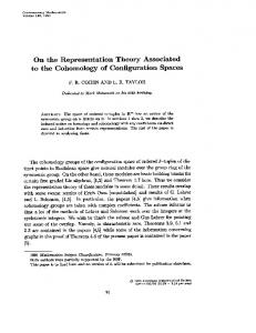
Figure 1. The proposed Bias Identification and Response Framework

a landscape of classifiers’ performance across different data assumption. Thus, our paper focuses on the following critical components relevant to an application of knowledge discovery and data mining process: a) detection of deviation in the predictive estimates over the testing set as compared to the validation set; b) identification of causes for such a drift in distribution that is what feature(s) are responsible for the testing population to change. We believe these issues are pervasive in the real-world deployment and evaluation of data mining solutions.

2 Bias in Data Sample selection bias [4, 5, 9, 24] provides our primary vehicle for establishing a violation of the stationary distribution assumption. Suppose that we consider examples (x, y, s) drawn independently from a distribution D where the domain is X × Y × S, with X being the feature space, Y is the class label space, and S is a binary space for which the variable s indicates the example is in the training when s = 1 and is not in the training set when s = 0. Operating in this environment, the following cases emerge regarding the dependency of s on (x, y) [9, 15].

Contribution This paper outlines a statistical framework, as depicted in Figure 1, to identify the fracture in predictive distributions and biases in feature space. We consider changes in data distribution by injecting scenarios of sample selection bias. We approach the problem in two stages. In stage one, we detect whether there is a statistically significant shift in the predictive distributions. We propose to use the Kruskal-Wallis test [7] to isolate bias through the distribution of probabilities generated by a learning algorithm. Note that the tests are unsupervised as we will not be aware of the actual testing set classes. Thus, we compare the posterior probability distributions between the validation set and testing set. If this test indicates that there is indeed a shift in the predictive distribution, a practitioner may then use a series of unsupervised statistical measures based on the Kolmogorov-Smirnov Test [11, 20] and Hellinger Distance [2] to indicate the presence or absence of bias in the

Definition 2 The missing completely at random (MCAR) sample selection bias occurs when s is independent of both x and y. We thus state that P (s = 1|x, y) = P (s = 1), thus the sample bias depends on a factor totally independent from the feature vector x and class label y. This implies that the training and testing sets are derived from the same distribution. The stationary distribution assumption theoretically holds under MCAR, but we include it in our paper for completeness. Definition 3 Sampling bias is missing at random (MAR) if s depends on x but conditional on x is independent of y, thus, we may state P (s = 1|x, y) = P (s = 1|x). Therefore, sampling is feature dependent as the sampling proba-

124

Dataset Compustat E-State Mammography Oil Page Pendigits Phoneme Satimage Segment

Examples (7,400, 2,958, 3,299) (2,662, 1,064, 1,596) (5,593, 2,236, 3,354) (470, 188, 279) (2,738, 1,094, 1,641) (5,497, 2,198, 3,297) (2,702, 1,081, 1,621) (3,218, 1,287, 1,930) (1,155, 462, 693)

3 Datasets and Classifiers

Features 20 12 6 49 10 16 5 36 19

This paper uses several common UCI [16] and realworld datasets, summarized in Table 1. These datasets vary extensively in both size and distribution, offering many different domains. Page, Pendigits, Phoneme, Satimage, and Segment come from the UCI Machine Learning repository [16]. The Oil dataset contains a set of oil slick images based on live data [12]. Compustat represents real world finance data and may contain natural bias as the training and testing samples come from different two-year periods, while Mammography comes from studying calcifications in the medical domain [22]. E-State consists of electrotopological state descriptors for a series of compounds from the National Cancer Institute’s Yeast AntiCancer drug screen [8].

Table 1. Datasets used in this study. Column Examples indicates the number of examples given as (training, validation, testing)

For the experiments conducted, we used C4.5 Decision Trees, Naive Bayes, k-Nearest Neighbor (where k = 5), and Support Vector Machines. Each classifier formed probability estimating models. Decision trees were trained as Probability Estimation Trees (PETs) [17]. k-Nearest Neighbor formed predictive probabilities as the proportion of the classes for the set of nearest neighbors. For SVM, the SVMlight software [1] was used with default parameters to form probabilistic predictions. Naive Bayes naturally forms probabilities. We restrained ourselves to default parameters for all classifiers to establish an even playing-field.

bility varies according to the feature vector x, but is independent to the class label y. This situation can occur if the testing set is thresholded on one or more known features.

Definition 4 Missing not at random (MNAR) bias occurs when there is no independence assumption between x, y, and s. This scenario essentially introduces the sample selection bias, as the cause of distributional shifts may be unknown. That is, one may not have access to the feature leading to the censoring in the dataset. We may state the tautology of P (s = 1|x, y)
= P (s = 1|x). Thus, at any particular feature x, the distribution of observed y in the training set is different from the observed y in the testing set – P (y = 1|x, s = 1)
= P (y = 1|x, s = 0).

4 Effect of Bias on Classification Various factors can be responsible for introducing distributional divergences in the testing set. The feature space could be biased through a number of methods, causing the classifier to generate inappropriate predictive distributions. In some cases, bias occurs as a result of collecting separate sub-populations governed by independent feature and class probability density functions within a single distribution. An example is the frequencies of measured wingspans of one species of bird found on two independent tropical islands. Temporal distance may also incorporate bias: the rules governing data may change slightly or drastically over time. Such biases can occur in various applications such as marketing and credit scoring, as the targeted population can change over time.

We establish the biases as follows. MCAR is used to remove 25% and 50% of the testing set; the examples are removed uniformly at random. We also use MAR and MNAR by removing the top 25% and 50% of values along one feature. We first sort the dataset based on one particular feature and then remove the top 25% or the top 50% of examples conditioned on that particular feature. In the case of MNAR, the remaining examples have the selected feature masked as “Unknown”. This incorporates a significant bias, as a substantial portion of the distribution is removed. By masking the feature as unknown or missing, we are able to inject the “latent” MNAR bias. We generate separate MAR and MNAR biased testing distributions for each feature within the dataset and the reported results within this paper are aggregates to indicate the “average case” for bias introduction. For fairness, an equivalent number of MCAR samples were generated; thus, MCAR results are similarly aggregated.

We now present a case study across classifiers and different datasets to demonstrate the effect of biases in the testing set. We use the Friedman test to statistically validate whether the predictions in the testing set start to significantly differ from the validation set once the biases are introduced. We will discuss the Friedman test before presenting our results.

125

1

Tree Bayes kNN SVM

Friedman p−value

0.8

0.6

0.4

0.2

0 Base

MCAR25

MCAR50

MAR25

MAR50

MNAR25

MNAR50

Figure 2. Friedman Test p-values across all datasets. +’s represent the average p-value.

4.1

Friedman Test

We introduced the three biases — MCAR, MNAR, and MAR — as follows. Considering a feature for each data set at a time, we injected the corresponding amounts of biases as discussed in the previous section. This resulted in as many testing sets as the number of features for each dataset and bias combination. This allowed us to avoid the dominance of results by any one feature in particular. We applied the same classifiers learned on the training set to each of the generated biased testing sets resulting in probabilistic predictions. Then, we formed 100 bootstraps on each (validation and testing) set of probabilistic predictions for each dataset and calculated accuracies on each. The Friedman test was then used to test the null hypothesis: there is no statistically significant difference between the validation and testing set accuracies for a dataset. Figure 2 shows the resulting p-values. The p-values for a given amount of bias are the averages of the p-values from the application of that particular bias to each feature in the dataset. Thus, it reflects the summarized p-value given a bias, dataset, and classifier. The convention in the figure is: the x-axis domain shows the different testing biases, including the Base stationary distribution. Each bias has a cluster of four lines representing the different classifiers. The y-axis shows the range of p-value across all the datasets for each classifier. As the p-value decreases, the hypothesis is more strongly rejected. Figure 2 shows a compelling trend. If we run along the xaxis, we observe that the range drops as we go more towards heavily biased testing sets. This confirms the premise that the performances of classifiers will suffer in non-stationary environments. Among the classifiers, decision trees and knearest neighbor seem to be less sensitive to distributional biases as compared to SVM and Naive Bayes. Since the yaxis reflects the range over datasets, we observe that some datasets lead to a complete failure of predictive estimates (pvalue of approximately 0). Nevertheless, within 85% confidence all the classifiers fail for all the datasets at MNAR-50. This is a strong demonstration of the fragility of classifiers in changing distributions, hence the forming the main motivation of our work.

The Friedman test is a non-parametric statistical test developed by the U.S. economist Milton Friedman [14]. The Friedman test is used for two-way analysis of variance by ranks. This two-way test assumes that all data comes from populations having the same continuous distribution, apart from possibly different locations due to column and row effects and that all observations are mutually independent. An example Friedman test evaluation is of n welders using k welding torches with the ensuing welds were rated on quality. Is there one torch that produced better welds than the others? X is a matrix such that observances are placed in columns and samples are stored across rows. r(xij ) is then the rank within block (i.e. within its row). The average rank per sample is calculated as rj =

k


r(xij )

(1)

i=1

k is the number of samples and n represents the number of examples in each sample. With the above ranking, calculate the following: k

χ2 =


12 r2 − 3n(k + 1) kn(k + 1) j=1 j

(2)

with χ2 as an associated p-value. This is the p-value for the null hypothesis that the column medians are essentially the same. When the p-value is very low, this indicates that this is likely not the case and the null hypothesis is void. To apply Friedman, we begin by first randomly partitioning the dataset into 50% for training, 20% for validation, and 30% for testing. Each classifier learned on the corresponding training set is then applied to the natural validation and testing samples, resulting in probabilistic predictions on both sets. This formed the Base results for the stationary distribution assumption, that is both validation and testing sets were derived from the same distribution.

126

1

Tree Bayes kNN SVM

Kruskal−Wallis p−value

0.9 0.8 0.7 0.6 0.5 0.4 0.3 0.2 0.1 0

Base

MCAR25

MCAR50

MAR25

MAR50

MNAR25

MNAR50

Figure 3. Kruskal-Wallis Test p-values across all datasets. +’s represent the average p-value. same. This test calculates the following statistic g n (¯ r − r¯)2 nii i K = (N − 1) g i=1 ¯)2 j=1 (rij − r i=1

We note that one can directly use this framework to generate biases during the validation process. This can result in an immediate evaluation of sensitivity of different classifiers as the population drifts. Then, conditioned on the nature of the application, one can then choose a classifier that is most consistent, perhaps at the cost of some accuracy at the stationary distribution.

where ng is the number of observations in group g, rgj is the overall rank of observation j in group g, N is the total number of observations, r¯g is the average rank of the observations within group g, and r¯ is the average rank of all observations. The p-value is then calculated as

5 Detecting and Identifying Bias

Pr(χ2g−1 ≥ K)

The goal of this work is to apply unsupervised methods to detect bias. Unsupervised methods are required as the class of testing data is presumed to be unknown at the time of evaluation. The following subsections provide tests for finding bias through three separate tests: the KruskalWallis Test in Section 5.1, the χ2 test for nominal features in Section 5.2 and the Kolmogorov-Smirnov test for continuous features in Section 5.3, and Hellinger Distance in Section 5.4. Together, they provide a statistical framework as shown in Figure 1. We have split the original data into the 50 : 20 : 30 training, validation, and testing proportion, respectively, as described before. We introduce MAR and MNAR onto each feature independently to form a separate testing sample and MCAR to generate the same number of testing samples. The results in Sections 5.1, 5.3, and 5.4 all represent the average values found across bias on all features. This reflects the “average case” feature becoming biased in a particular dataset.

5.1

(3)

(4)

This is the p-value of the null hypothesis that all samples are drawn from the same population or different populations of the same distribution. Therefore, this is a very useful test for determining if sets of probabilities are drawn from the same or different distributions. Here it is applied as a comparison of the probabilities estimated on the validation set against the natural testing distribution and the six other biased distributions. In Figure 3 we observe the calculated set of KruskalWallis p-values. Those generated in comparing the set of validation probabilities against those of the testing set and distributions formed through MCAR are quite similar, which is expected as there is similarity between the validation sample and the testing and completely randomly biased testing samples. However, there is a substantive difference to the MAR and MNAR biased sets. Under these sophisticated biases, the distribution of probability estimates differs significantly. With such a drastic change in the estimates, there should follow a fairly substantial change in the classifier performance. We also note that the values captured through Kruskal-Wallis are quite correlated to those found under the supervised (determining accuracy and rank-order requires known classes) Friedman test (Figure 2). With this information, it is both feasible and useful for the practitioner to initially train a model and predict probabilities on both the validation and testing data samples. Using Kruskal-Wallis, the practitioner may then determine

Kruskal-Wallis Analysis of Generated Probability Estimates

Kruskal-Wallis one-way analysis of variance by ranks is a non-parametric method for testing equality of population medians among groups [7]. Unlike One-way ANOVA, no assumption regarding a normal distribution is made since the test is non-parametric. There is also no assumption that the population variables between compared groups are the

127

KS Test Comparison Cumulative Fraction Plot

whether the the sets of probabilities came from different populations. If so, it is then wise to use the tests in Sections 5.3 and 5.4 to attempt to determine bias type and isolate biased features.

0.9

Cumulative Fraction of X

5.2

1

χ2 Test

χ2 is a statistical test used to compare observed nominal data. This is useful in determining whether the distribution of observations within categorical data are dissimilar. χ2 =

p
v
i=1 j=1

ni,j N

− nˆj nˆj

(5)

Distribution A Distribution B

0.6 0.5 0.4

D

0.3 0.2

0 −3

−2

−1

0

1

2

3

4

5

6

7

X Figure 4. An example KS test plot. Here, the distributions are significantly divergent as D = 0.5.

(6)

2

than x. Figure 4 contains a plot of A against B. Using a planesweep, the KS test then calculates the maximum vertical deviation between the two distributions. For A and B, Figure 4 indicates this as D. In this case, the maximum vertical deviation is 0.5. We would like to state whether this value represents a significant distance. We calculate

Based on the found values of χ and df , a look-up table is then used to determine a p-value. With this test, we may determine an appropriate p-value for nominal features.

5.3

0.7

0.1

when there are p populations and v values, np,v represents the count of value v in population p, np is the p count within population p, N = n and nˆj = k k=1 p k=1 nk,j nk /N . We note that as we are comparing two distributions, p = 2. To determine a p-value with this test, degrees of freedom are also considered as df = (p − 1)(v − 1)

0.8

Kolmogorov-Smirnov Test

The Kolmogorov-Smirnov test (often called the KS test) determines if there is divergence between two underlying one-dimensional probability distributions or whether an underlying probability distribution differs from a hypothesized distribution, in either case based on finite samples [11, 20]. The two-sample KS test is particularly useful as a general nonparametric method of comparing two sample distributions as it detects divergence in both location and shape of the observed distribution functions. KS has an advantage over other statistical methods in that it makes no assumption on the distribution of data, which other methods such as Student’s t-test make. However, other methods may be more sensitive if the distributional assumptions are met. Quite simply, KS makes use of a plot of the Cumulative Fraction Function. Suppose we have two distributions, such that A = { 0.34, 0.94, 0.24, 1.26, 6.98, 0.95, 0.15, 2.08, 0.17, 1.55, 3.20, 0.50, 0.70, 4.55, 0.10, 0.49, 0.38, 0.42, 1.37, 1.75} and B = { 0.15, -0.62, -0.17, -0.31, -0.50, 0.38, 2.30, 0.37, -1.79, -0.87, 1.72, -0.09, -1.54, 0.30, -2.39, -0.74, 0.22, 1.28, 0.19, -1.10}. The KS test begins by sorting both sets of values independently. A single plot of both distributions is then generated. The x-axis contains the values of distribution. For each point x, the y-axis is calculated as the percentage of instances strictly smaller than x; hence, it is the cumulative fraction of the data which is smaller

χ2 =

4D2 n1 n2 n1 + n2

(7)

where n1 and n2 are the number of examples in the two samples. Using d = 2 and the χ2 calculation, the resultant p-value suggests whether there is a significant difference between the two distributions and may be compared against a desired confidence level. Within the context of data-mining, we may use the KS test to determine if there is a significant distributional difference between the training and testing distributions for continuous features. When features are nominal, a χ2 test is instead applied to determine p-value. To do so, we must iterate through both distributions on a feature wise basis, and tabulate the number of failing features, which is why using Kruskal-Wallis on the probability distributions is a better first step. Table 2 represents the proportion of features failing the KS test under each bias. Based on these results, we observe that Compustat, Page, and Segment contain some degree of natural bias between training and testing distributions. Of these, Compustat is the least surprising as its training and testing data come from two independent sets of financial information covering separate and sequential two year periods. For these three datasets, it is noted that MCAR actually reduces the fail-

128

Dataset compustat estate Mammography oil page pendigits phoneme satimage segment

Base 0.400 0.000 0.000 0.000 0.300 0.000 0.000 0.000 0.053

MCAR 25 0.367 0.000 0.028 0.004 0.190 0.004 0.000 0.000 0.022

MCAR 50 0.347 0.007 0.028 0.005 0.100 0.027 0.000 0.000 0.033

MAR 25 0.552 0.125 1.000 0.266 0.560 0.461 0.520 0.875 0.421

MAR 50 0.672 0.174 1.000 0.397 0.590 0.523 0.600 1.000 0.446

MNAR 25 0.529 0.083 1.000 0.252 0.511 0.425 0.400 0.871 0.395

MNAR 50 0.655 0.136 1.000 0.386 0.544 0.492 0.500 1.000 0.421

Table 2. Proportion of features failing the KS test at 95% confidence Dataset compustat estate Mammography oil page pendigits phoneme satimage segment

MCAR25 0.046 ± 0.003 0.000 ± 0.000 0.000 ± 0.000 0.001 ± 0.000 0.114 ± 0.028 0.000 ± 0.000 0.000 ± 0.000 0.000 ± 0.000 0.002 ± 0.000

MCAR50 0.053 ± 0.004 0.000 ± 0.000 0.000 ± 0.000 0.004 ± 0.000 0.156 ± 0.014 0.069 ± 0.006 0.000 ± 0.000 0.000 ± 0.000 0.009 ± 0.001

MAR25 0.391 ± 0.003 0.175 ± 0.021 0.000 ± 0.000 0.554 ± 0.004 0.461 ± 0.069 0.405 ± 0.003 0.467 ± 0.016 0.037 ± 0.001 0.311 ± 0.003

MAR50 0.217 ± 0.017 0.128 ± 0.016 0.000 ± 0.000 0.388 ± 0.002 0.399 ± 0.054 0.362 ± 0.020 0.349 ± 0.026 0.000 ± 0.000 0.235 ± 0.011

MNAR25 0.361 ± 0.026 0.104 ± 0.013 0.000 ± 0.000 0.476 ± 0.003 0.554 ± 0.069 0.453 ± 0.001 0.783 ± 0.069 0.051 ± 0.001 0.235 ± 0.014

MNAR50 0.250 ± 0.021 0.057 ± 0.007 0.000 ± 0.000 0.400 ± 0.003 0.479 ± 0.052 0.412 ± 0.013 0.650 ± 0.074 0.014 ± 0.000 0.249 ± 0.006

Table 3. Average φ-correlation for feature failure ure proportion somewhat, likely because there are unusual values creating large maximum separations. The random bias removes these values and reduces the separation, hence dropping the feature failure rate. In the remaining datasets, MCAR very minimally increases the feature failure rate, if at all. It is observed that the more systematic biases MAR and MNAR increase the feature failure rate substantially. This indicates that the KS test may be used simply and quite effectively to detect a bias incorporated between two data distributions. In addition to understanding the degree to which bias causes feature failure under the KS test, we seek to study the interaction of a particular feature failing on other features. Restated, Do features tend to fail independently or concomitantly? To this end, a Failure Correlation Matrix F was constructed where Fi,j represents the count for which features i and j fail under KS concomitantly. Based on the counts within F , the φ-correlation is calculated for each pairwise set of features as

chotomies and discounts the effects of sample size. The average correlation per pairwise comparison is reported in Table 3. Values between 0.0 and 0.3 are considered to have little to no associativity, 0.3 to 0.7 have some associativity, and above 0.7 has very strong associativity. The average φ-correlation is quite low, if not zero, for the baseline comparison and MCAR. Thus, there is little correlation between the failure of features, if failure occurs at all. As MAR and MNAR are introduced, there is a spike in φ-correlation. This is an expected result as there is some degree of covariance among the measured features; thus, a bias on one feature will to some degree incorporate a bias to related features. The exception to this trend is Mammography, which reports zero correlation categorically, as within each test either all or none of the features fail the KS test except for some MCAR trials for which failure occurred totally at random. We have thus demonstrated how the KolmogorovSmirnov Test may be used in identifying the proportion of features which are significantly different within two data samples. A more difficult bias usually causes a greater proportion of features to fail KS. In addition, we have combined KS with φ-correlation to determine how features fail independently and concomitantly under different bias. Once bias is suspected through the Kruskal-Wallis test

Fi,i Fj,j − Fi,j Fj,i φ=  (Fi,i + Fi,j )(Fi,j + Fj,j )(Fi,i + Fj,i )(Fj,i + Fj,j ) (8) as φ is a strong measure of the associativity of two di-

129

Hellinger Distance Percent Increase Over Baseline

700 MCAR25 MCAR50

600

MAR25 MAR50

500

MNAR25 400

MNAR50

300 200 100 0

Compustat

Estate Mammograph

Oil

Page

Pendigits

Phoneme

Satimage

Segment

Figure 5. Hellinger Distance detecting bias. From left to right each set of bars indicates the relative change in Hellinger Distance between the testing sample and MCAR25, MCAR50, MAR25, MAR50, MNAR25, MNAR50 for each dataset.

dependent distributions of data X and Y . Both X and Y contain p bins, where each bin contains the count of some logical subunits measured between X and Y . The Hellinger Distance between X and Y is then calculated by

on the set of predicted probabilities, the KS Test operates as a “quick” method to check for the existence of bias to see if a fairly high proportion of the features fail this test (in most cases, 30% feature failure appears to be a reasonable point to presume some bias as observed in Table 2). Table 3 reported the φ-correlation of the KS Test as capable of determining groups of features which tend to fail together. Suppose there is a high correlation of failure between two features. In the case that only one fails, one may assume a reasonable correlation between the two features and omit the failing feature during model training confident that the succeeding feature will account for much of the information contained within the failing one. As seen in Table 2, the KS Test struggles to isolate individual biased features. Thus, it is a good method to confirm the findings from KruskalWallis. To more acutely determine degree and which features are biased, we turn to Hellinger Distance.

5.4

   2  
p  Xj Yj Hellinger(X, Y ) =  − |X| |Y | j=1

(9)

Suppose that there exist two populations, P op1 and P op2. The occurrence count of value a, b, and c within each population have been tabulated and are reported in Table 4.

P op1 P op2

a 7 0

b 0 10

c 0 2

Hellinger Distance Table 4. Example population data

Hellinger Distance [2], also referred to as Bhattacharyya Distance [10], is a measure of distributional divergence. [13] concludes that for linear ordination, the Hellinger Distance offers a better compromise between linearity and resolution, as compared to similar metrics such as the χ2 metric and the χ2 distance. Hellinger distance has been used effectively within the ecological domain and is recommended for clustering or ordination of species abundance data [18]. This measure has also been used as a means of locating statistical outliers for fraud detection in insurance applications[23]. To apply this measure of density, we presume two in-

√ Using (9), Hellinger(P op1, P op2) = 2, which happens to be the maximum possible Hellinger Distance. This is expected as P op1 and P op2 are completely divergent: there is no overlap in values a, b, and c. Hellinger Distance can be applied simply to each feature individually. In the case of nominal features, each feature value forms a separate bin. Hellinger then measures the difference between the counts of each value. Continuous features are treated similarly through discretization by 30 equal-width bins. For each dataset, the average per feature

130

Dataset Compustat E-State Mammography Oil Page Pendigits Phoneme Satimage Segment

MCAR 25 -0.790 -0.195 0.634 0.957 -0.609 -0.271 -0.171 -0.097 -0.656

MCAR 50 -0.751 -0.055 0.466 0.911 -0.253 -0.836 0.049 -0.127 -0.445

MAR 25 -0.562 -0.349 -0.332 0.868 -0.239 -0.283 -0.095 -0.008 0.134

MAR 50 -0.554 -0.618 -0.021 1.007 -0.137 -0.413 -0.002 -0.025 0.092

MNAR 25 -0.554 -0.715 -0.179 1.131 -0.103 -0.161 0.527 0.010 0.306

MNAR 50 -0.545 -1.115 0.274 1.183 -0.060 -0.295 0.448 -0.001 0.272

Table 5. Skew of the average Hellinger Distance per feature

6 Conclusions

Hellinger Distance is then calculated. The observed relative changes from the distance calculated on the base testing distribution are summarized in Figure 5. The calculated distances tend to be relatively low between the base training and testing distributions and testing distributions generated through MCAR. There is a substantial increase in Hellinger Distance when an MAR or MNAR is at play. Thus, applying Hellinger Distance is quite effective in differentiating between the relative level of bias sophistication.

Data mining is presented with the challenge of drifts in data distribution between the training and testing samples. The basic assumption that the past is a reasonable predictor of future may not hold in different scenarios. This certainly hinders the performance of learning algorithms, as we have also demonstrated in this work. Thus, it becomes critical to identify and react to the changes in data distribution. To that end, we implemented a framework that comprised of a family of statistical measures. We showed that it is possible to proactively detect fractures in classifier performance. Our test suite comprised of a variety of classifiers and data sets with different characteristics. Based on our observations, we make the following recommendations. Using Kruskal-Wallis on the distributions of validation and testing probabilities is useful as a first step. If the practitioner determines there is no significant difference between them, then it is possible to proceed as per typical. Otherwise, the practitioner should use the following tests to isolate biased features. The Kolmogorov-Smirnov Test ably detects independent feature failure. Through φcorrelation analysis, KS also determines the co-failure of features, which is quite strong under sophisticated bias. Hellinger Distance is also quite useful as it readily identifies and differentiates the level of bias, even when the factor of bias is unmeasured, such as MNAR. When the cause of bias is known, a high skew in Hellinger Distances is indicative that it is capable of isolating features generating bias between samples. We believe that a single statistical measure cannot be used in isolation, rather a family of measures should be used in conjunction to remain more confident in detecting fractures in classifier predictions.

Of additional interest is the skew of Hellinger Distances produced. In fact, Table 5 demonstrates that there is typically a substantial negative skew to the set of distances calculated, meaning there is a tail of values below the mean. This is indicative that is more data below the mean than would be expected in a normal distribution. There are a few very high distances shifting the mean upwards causing the lower distance values to be further from the mean than in a normal population. We note that Oil violates this trend, likely due to the extremely small size of this dataset. In general, Hellinger Distance enables the isolation of features along which bias occurs. From these experiments, we note that Hellinger is able to corroborate the findings of KS and complements the differentiation and determination of biases. The KS Test is useful in determining if there is a significant maximal point of separation. Hellinger Distance is more refined in isolating bias since it is a method of comparing the relative densities of two distributions. MCAR is the lowest range, then MNAR, then MAR. We expect this ordering: MCAR is sampled at random and should fairly closely resemble the training set. MAR should produce the highest changes in Hellinger: the feature(s) generating bias have been observed and the distributional change will be reflected by this distance. MNAR is expected to produce results between MCAR and MAR since the feature MNAR biases along is hidden, but it is also reasonable to expect some level of correlation to the observed features. We recommend a coupled usage of KS test and Hellinger distance to isolate the biased features.

References [1] SVMlight Support Vector Machine. http://www.cs.cornell.edu/People/tj/svm light/.

131

[15] R. Little and D. Rubin. Statistical Analysis with Missing Data. Wiley, New York, 1987.

[2] A. Basu, I. R. Harris, and S. Basu. Minimum distance estimation: The approach using density-based distances. In Handbook of Statistics, volume 15, pages 21–48, 1997.

[16] D. Newman, S. Hettich, C. Blake, and C. Merz. UCI Repository of Machine Learning Databases, 1998.

[3] R. Caruana and A. Niculescu-Mizil. Data Mining in Metric Space: An Empirical Analysis of Suppervised Learning Performance Criteria. In Proceedings of the Tenth International Conference on Knowledge Discovery and Data Mining (KDD’04), pages 69–78, 2004.

[17] F. Provost and P. Domingos. Tree Induction for Probability-Based Ranking. Machine Learning, 52(3):199–215, September 2003. [18] C. Rao. A Review of Canonical Coordinates and an Alternative to Corresponence Analysis using Hellinger Distance. Questiio (Quaderns d’Estadistica i Investigacio Operativa), 19:23–63, 1995.

[4] N. V. Chawla and G. Karakoulas. Learning From Labeled And Unlabeled Data: An Empirical Study Across Techniques And Domains. JAIR, 23:331–366, 2005.

[19] J. Shawe-Taylor, P. Bartlett, R. Williamson, and M. Anthony. A Framework for Structural Risk Minimisation. In Proceedings of the 9th Annual Conference on Computational Learning Theory, 1996.

[5] W. Fan and I. Davidson. ReverseTesting: An Efficient Framework to Select Amongst Classifiers under Sample Selection Bias. In Proceedings of KDD, 2006.

[20] N. Smirnov. On the estimation of the discrepancy between empirical curves of distribution for two independent samples. (Russian) Bulletin of Moscow University, 2:3–16, 1939.

[6] W. Fan, I. Davidson, B. Zadrozny, and P. Yu. An Improved Categorization of Classifier’s Sensitivity on Sample Selection Bias. In 5th IEEE International Conference on Data Mining, 2005.

[21] V. Vapnik. The Nature of Statistical Learning. Springer, New York, 1996.

[7] J. D. Gibbons. Nonparametric Statistical Inference, 2nd edition. M. Dekker, 1985.

[22] K. Woods, C. Doss, K. Bowyer, J. Solka, C. Priebe, and W. P. Kegelmeyer. Comparative Evaluation of Pattern Recognition Techniques for Detection of Microcalcifications in Mammography. IJPRAI, 7(6):1417– 1436, 1993.

[8] L. Hall, B. Mohney, and L. Kier. The Electrotopological State: Structure Information at the Atomic Level for Molecular Graphs. Journal of Chemical Information and Computer Science, 31(76), 1991.

[23] K. Yamanishi, J. ichi Takeuchi, G. J. Williams, and P. Milne. On-line unsupervised outlier detection using finite mixtures with discounting learning algorithms. In Knowledge Discovery and Data Mining, pages 275–300, 2004.

[9] J. J. Heckman. Sample Selection Bias as a Specification Error. Econometrica, 47(1):153–161, 1979. [10] T. Kailath. The Divergence and Bhattacharyya Distance Measures in Signal Selection. IEEE Transactions on Communications, 15(1):52–60, February 1967.

[24] B. Zadrozny. Learning and Evaluating under Sample Selection Bias. In Proceedings of the 21st International Conference on Machine Learning, 2004.

[11] A. N. Kolmogorov. On the empirical determination of a distribution function. (Italian) Giornale dell’Instituto Italiano degli Attuari, 4:83–91, 1933. [12] M. Kubat, R. Holte, and S. Matwin. Machine Learning for the Detection of Oil Spills in Satellite Radar Images. Machine Learning, 30:195–215, 1998. [13] P. Legendre and E. D. Gallagher. Ecologically Meaningful Transformations For Ordination Of Species Data. Oecologia, 129:271–280, 2001. [14] H. R. Lindman. Analysis of variance in complex experimental designs. W. H. Freeman & Co., San Francisco, 1974.

132