tree clearing and present a solution for finding paths for the robot team that ensure the detection of all intruders with a proven upper bound on the number of ...
Detecting intruders in complex environments with limited range mobile sensors. Andreas Kolling and Stefano Carpin University of California, Merced School of Engineering – Merced,CA, USA
Summary. This paper examines the problem of detecting intruders in large multiplyconnected environments with multiple robots and limited range sensors. We divide the problem into two sub-problems: 1) partitioning of the environment and 2) a new problem called weighted graph clearing. We reduce the second to a weighted tree clearing and present a solution for finding paths for the robot team that ensure the detection of all intruders with a proven upper bound on the number of robots needed. This is followed by a practical performance analysis.
1 Introduction Multi-target surveillance by a team of mobile robots as one of the more active and novel research areas in robotics has received particular attention in recent years. Its core problems are at an interesting cross-section between path-planning, map building, machine learning, cooperative, behavioral and distributed robotics, sensor placement and image analysis. We are currently investigating the problem of detecting intruders in large and complicated environments with multiple robots equipped with limited range sensors. The problem is closely related to pursuit-evasion and cooperative multi-robot observation of multiple moving targets, short CMOMMT, which we are going to discuss shortly in section 2. The main contribution of this paper is to present a starting point for an approach for a team of robots with limited range sensors. We divided the initial problem into two sub-problems: 1) to partition the environment into a graph representation and 2) to clear the graph from all possible intruders with as few robots as possible. For the remainder of this paper we are going to focus on the later problem. Interestingly, the division has the effect that we can present an algorithm to compute a clearing strategy on the graph without considering the robots’ capabilities directly. Hence with some further work the algorithm is extendable to teams of heterogeneous robots. The clearing strategy consists of paths for the robots on the vertices and edges of the graph. When executed it ensures
2
Andreas Kolling and Stefano Carpin
that any arbitrarily fast moving target present in the environment will be detected. To find a clearing strategy we need to solve a graph theoretical problem which we dub weighted graph clearing, introduced in section 3.1. In section 3 we provide a solution for the problem with a proven upper bound followed by some experiments in section 4. Finally, our results and and a outlook on the first sub-problem are to discussed in the section 5.
2 Related Work The two research areas most closely related to our work are CMOMMT and pursuit-evasion. CMOMMT is related due to its focus on multi-robot teams in large environments with sophisticated cooperation. The term was coined by Parker who produced the first formal definition of the problem and an algorithm in [2]. It focuses on multi-target surveillance in large environments with mobile robots with limited range sensors with the goal to optimized resource usage when resources are not sufficient to surveil all targets. Recent improvements were presented in [1] by introducing a new distributed behavioral approach, called Behavioral-CMOMMT. The improvements are due to an advanced cooperation schemes between robots which boost the overall performance. Pursuit-evasion is usually tackled from the perspective of the pursuer, i.e. the goal is to try to make impossible for the evader to escape. Most current solutions for this pursuit-evasion problem, however, require unlimited range sensors. In [3] an algorithm for detecting all targets in a subclass of all simply connected environments is presented. The restrictions on the subclasses are relatively few and the performance of the algorithm is proven. It guarantees to find a path to clear the environment of all targets using only a single pursuer with a gap sensor with full field of view and unlimited range. The drawbacks are frequently revisited areas and hence long clearing paths. In [4] and [5] a previous algorithm for a single pursuer is presented in more detail and in [4] interesting bounds on the number of robots required for certain free spaces are established. For simply-connected free spaces a logarithmic bound is obtained, while for a multiply-connected environment a bound in the square root of the number of holes is given. Furthermore, finding the number of robots needed to clear an environment was shown to be NP-hard. Gerkey et al. in [6] extended the previous algorithm to varying field of view. Pursuit-evasion solutions draws most of their information from a particular method of partitioning to finding a clearing strategy. This will be useful for extensions of this paper when the first sub-problem is discussed and related to the weighted-graph clearing problem. For now we shall present a solution that is independent of any partitioning but yet a powerful method in the divide and conquer spirit.
Detection of Intruders
3
3 The Algorithm To prepare the grounds for the algorithm we will define our notion of environment, regions, adjacency and contamination. An environment, denoted by S, is a bounded multiply connected closed subset of R2 . A region is a simply connected subset of S. Let r1 and r2 be two regions and let r¯1 and r¯2 denote their closures. If r¯1 ∩ r¯2 6= ∅, then we say that r1 is adjacent to r2 and vice versa. Let S g = {r1 , . . . , rl } be a partition of S with l regions. Let Ari be the set of all adjacent regions to ri . Define a binary function for each region ri on its adjacent regions and across time: bri : Ari × R → {0, 1}. Let rj ∈ Ari . If bri (rj , t) = 1 we shall say that the adjacent region rj is blocked w.r.t. ri at time t. Define another binary function: c : S g × R → {0, 1}. If c(r, t) = 1, then we shall call region r contaminated at time t, otherwise clear. Let Acri be the set of all contaminated adjacent regions to ri . Let c have the following property: ∀� > 0 : c(r, tc + �) = 0 ⇐⇒ c(r, tc ) = 0 ∧ b |Acr (t + �) = 1 i
(1)
Now, if c(r, tc ) = 0 and ∃� > 0 s.t. ∀t ∈ (tc , tc + �], c(r, t) = 1, then we say that that r is re-contaminated after time tc . These definitions give us a very practical notation for making statements about the state of regions. In particular, it follows that a region becomes recontaminated when it has a contaminated adjacent region that is not blocked. We are now going to define two procedures, called behaviors, which set the function c and b, i.e. enable us to clear and block. Definition 1 (Sweep and Block). A behavior is a set of instructions assigned to one or more robots. The two behaviors are defined as follows: 1. Sweep: a routine that detects all invaders in a region assuming no invaders enter or leave the region. After the execution of a sweep on a region r at time t we set c(r, t) = 0, i.e. not contaminated1 . 2. Block: a routine that ensures that no invaders enter from or exit to adjacent regions. For a region r a block is executed on an adjacent region ra in Ar . A block on ra is defined as covering the boundary of r intersected with ra with sensors, i.e. δ¯ r ∩ r¯a ⊂ sensor coverage, where sensor coverage is the area covered by all available sensors of all robots. Furthermore, let us denote a sweep as safe if and only if during the execution of the sweep we have b |Acr = 1. It follows that after a safe sweep a region i remains clear until a block to a contaminated region is released. All the previous can be understood as the glue that connects the two subproblems, partitioning and finding the clearing strategy. Partitioning returns the graph representation of the environment into which one can encode the 1
therefore we assume that when a robot detects and intruder, the intruder is neutralized and cannot operate anymore
4
Andreas Kolling and Stefano Carpin
number of robots needed for the behaviors on the edges, the blocks, and the vertices, the sweeps, by adding a weight to them. The values of the weigths are specific to the robots capabilities and methods used for sweeping and blocking. Depending on the partitioning, very simple methods can be used. We assume a homogeneous robot team from here on, which makes the interpretation of these weights easier and the notation for the following simpler to follow. We now define the main problem that we are going to investigate, i.e. weighted graph clearing. The task is to find a sequence of blocks and sweeps on the edges and vertices of an entirely contaminated graph such that the graph becomes cleared, i.e not contaminated, with the least number of robots. This sequence of blocks and sweeps will be our clearing strategy to detect all intruders. 3.1 Weighted graph clearing We are given a graph with weighted edges and vertices, denoting costs for blocks and sweeps. The goal is to find a sequence of behaviors to clear the graph using the least number of robots. As the first step we attempt to reduce the complexity of the problem by reducing the graph to a tree by removing occurring cycles. Cycles can be eliminated by executing a permanent block on one edge for each cycle. The choice of such edge will influence the tree structure and hence our final strategy. This is a topic that requires further investigation, as discussed in section 5. Recall the partition S g in form of a planar graph. Let the weights on the edges and vertices be denoted by w(ei ) on edges and w(ri ) on vertices and all be non-zero. The weight of a vertex is the number of robots needed to complete a sweep in the associated region, while the weight of an edge is the number of robots required to block it. To transform S g into a tree we compute the minimum-spanning-tree (MST) with the inverse of the w-weight of the edges. Let B be the set of all removed edges to get the MST. The P costs for blocking all edges in B and transforming S g into a tree is b(B) = ei ∈B w(ei ) and as such the minimum possible. From now on this cost is constant and will henceforth be ignored. 3.2 Weigthed tree clearing Recall that a safe sweep requires all adjacent regions to be blocked. It is clear that we have to block contaminated and cleared regions alike, since the latter may get re-contaminated. Hence for a safe sweep for a region ri we need s(ri ) = sumej ∈Edges(ri ) w(ej ) + w(ri ) robots. After a safe sweep all blocks on edges to cleared regions can be released. To remove the blocks to contaminated regions we have to clear these first. This suggests a recursive clearing of the regions. To capture this we define an additional weight on each edge, p(ej ), referred to as p-weight. For clarity: the p-weight for edges is the number of robots needed to clear the region accessible via this edge and all its sub-regions into the respective direction. Once we have the p-weight we
Detection of Intruders
5
still have to choose at each vertex which edges to visit first. Let us define the order by p(ej ) − w(ej ) with the highest value first. The following algorithm computes the p-weight and implicitly selects a vertex as the root which is the starting point for the clearing. For each region r, let Edges = {en1 , . . . , enm(r) } denote the set of edges. 1. For all edges ej that are edges to a leaf ri set p(ej ) = w(ej ) + w(ri ). 2. For all vertices ri that have its p-weight assigned for all but one edge, denoted by en1 , do the following: a) Sort all m − 1 assigned edges w.r.t to p(ej ) − w(ej ) with the highest value first. Let the order be en2 , . . . , P enm . b) Determine h := max2≤k≤m (p(eni ) + 1 1. W.l.o.g. assume that m ≥ 3, otherwise we have p(en1 ) = P max(p(en2 ), s(r)). Since s(r) ≤ hmax and s(r) = ej ∈Edges(r) w(ej ) + w(r) we get: X w(ei ) ≤ hmax − 2. ei ∈Edges(r)\{en1 }
Consider the worst case for the last edge P enm to be cleared from r. All other edges have to be blocked with cost ei ∈E 0 w(ei ) while we clear sub-regions beyond enm with cost p(enm ). Due to the ordering of edges we know that
6
Andreas Kolling and Stefano Carpin
p(enm ) − w(enm ) is smaller than for other edges. The worst case costs occur P when the p weight of enm is as big as possible while at the same time ei ∈E 0 w(ei ) is large. Trivially we have: X w(ei ) ≤ hmax − 3 ei ∈E 0
For p(enm ) we know: p(enm ) ≤ p(eni ) − w(eni ) + w(enm ) due to the ordering. Hence it follows that the worst case occurs when: p(enm ) = max(p(eni )), w(eni ) = 1, m = hmax − 2 So we get p(eni ) = p(enj ), ∀j, i > 1. A quick proof by contradiction shows that the last edge in the worst case is the worst edge. Now the bound for p(en1 ) if p(enm ) > 2 becomes: p(en1 ) ≤ p(enm ) + hmax − 3. (Note: if p(enm ) = 2 then we may get p(enm ) + hmax − 3 = hmax − 1 and violate that possibly p(en1 ) = s(r) = hmax ) We can now use this to derive a bound for the entire tree. We start with the leaves at worst case hmax for a safe sweep, so all p-weights at the first stage are hmax . Now we assume the worst case for all other vertices. This gives us: max g {p(e)} ≤ hmax + (d∗ − 1) · (hmax − 3) e∈Edges(S )
� The number of robots needed can easily be computed by adding a ”virtual” edge to the root vertex and computing its p-weight. Figure 1 illustrates a worst case example with d = 6, hmax = 6 and the resulting size of the robot team of 16. The actual exploration proceeds by choosing the subtree with the highest p(ei ) − w(ei ) first, then once it is explored blocking it and continuing with the new one in order until the last subtree is cleared. The example from figure 1 is generic and establishes the bound as tight for any d and hmax . It, however, only occurs in exactly such an example in the sense that we need all vertices and leaves to have exactly the structure for the worst case as indicated in the proof and figure. When seeking the optimal root vertex for the deployment one can use the same principal method and calculate p-weights in both directions, append a virtual edge to each vertex and then choose the vertex with the smallest p-weight for this virtual edge.
4 Investigation of Performance To show the practicability of the algorithm we ran the recursive sweep on randomly generated weighted trees. Trees with 20, 40, 60, 80 and 100 vertices,
Detection of Intruders 5 400
5
7
1:6
1:6
●
deploy 16 robots 1:12
1:12
1:9
1
1:9
●
200
1:9
●
300
5 Average maximum of p
1:9 1:12
1:6
1
●
●
100
1:6
Actual values Upper bound
1 1:12
●
●
20
40
●
●
●
60
80
100
0
5
1:12
Number of vertices
Fig. 1. This is the worst case example for d = 6, hmax = 6, p∗ = 6+2·3 = 12. Blocking weight w is indicate left and p-weight right of : on the edge. Each vertex has its weight in its center.
Fig. 2. A comparison of the average upper bound across 1000 weighted trees and actual maximum p-weight for varying number of vertices.
random edges, a random weight for a vertex between 1 and 12 and a random weight for edges between 1 and 6 were generated. For each number of vertices a forest of 1000 trees was created. The average values for the maximum pweight, d∗ and hmax are presented in table 4. Figure 2 compares the upper bound computed from d∗ and hmax with the average maximum value of p. n Vertices max(p(e)) d* hmax 20 24.865 5.325 25.176 40 28.300 7.784 27.949 60 30.299 9.638 29.607 80 31.781 11.077 31.039 100 32.885 12.306 31.909 Table 1. Results of the experiments. Values are averaged across 1000 random trees. The max(p(e)) is the largest p-weight occuring in the tree, without any virtual edges attached, while hmax is the largest s-weight of the vertices. Note that if the root has the largest s-weight it may be that hmax > max(p(e)), which is often the case with smaller trees since the root on average has the most edges.
5 Discussion and Conclusion We presented a first approach for a complex problem and started at dissecting it into the two sub-problems that can be paraphrased into the two major
8
Andreas Kolling and Stefano Carpin
challenges of understanding the environment and then coordinating the team effort. We presented a solution to coordinate the team effort with a central instance by solving the weighted graph clearing problem. The benefit is that we can now partition an environment into many simple regions for which one can easily find a sweeping routine for limited range sensors. Particularly suitable are environments such as buildings for which we would suggest a partitioning into regions that are rooms and hallways. The sweeping of a room can then be done by aligning the robots, and then the sensors, on a line. On our path towards a fully working system there are two sets of questions arising. The first set are those regarding the theoretical part, i.e. solving the graph clearing problem without using the heuristic of the constant cycle blocks. First of all, choosing the cycle blocks defines the tree structure and hence influences the resulting strategy. We might get a better strategy if we choose the block w.r.t. to this criteria. Secondly, once we have cleared two regions connected by an edge that has a cycle block it becomes redundant. We could free the block and gain resources and we would want to free these additional resources exactly when we need them, namely when we enter regions with high weights. The second set of questions are those regarding the partitioning. One needs to determine good methods for partitioning depending on the environment and capabilities of the robots. Also we need to conceive criteria for partitions that lead to good strategies on the graph. A first hint of the theorem is that deep trees should be avoided. Understanding the theoretical properties of the weighted graph clearing problem first, might already give us good insight on how to start creating good partitions. Then we can work on devising good partition strategies in coordination with sweeping and blocking methods for particular sensors and close the loop to a working system.
References 1. A. Kolling, S. Carpin, “Multirobot Cooperation for Surveillance of Multiple Moving Targets - A New Behavioral Approach,” Proceedings of the 2006 IEEE International Conference on Robotics and Automation, pp. 1311–1316 2. L. E. Parker, “Distributed algorithms for multi-robot observation of multiple moving targets,” Autonomous robots, 12(3):231–255, 2002. 3. S. Sachs, S. Rajko, S. M. LaValle. “Visibility-Based Pursuit-Evasion in an Unknown Planar Environment,” The International Journal of Robotics Research, 23(1):3-26, 2004 4. L. J. Guibas, J. Latombe, S. M. LaValle, D. Lin, R. Motwani, “Visibility-Based Pursuit-Evasion in a Polygonal Environment,” International Journal of Computational Geometry and Applications, 9(5):471–494, 1999 5. S. M. LaValle, D. Lin, L. J. Guibas, J. Latombe, R. Motwani, , “Finding an Unpredictable Target in a Workspace with Obstacles,” Proceedings of the 1997 IEEE International Conference on Robotics and Automation, pp. 737–724 6. B. P. Gerkey, S. Thrun, G. Gordon. “Visibility-based pursuit-evasion with limited field of view,” The International Journal on Robotics Research, 25(4):299316, 2006.