Mar 25, 2012 - The deflection angle depends on the particle velocity and ... their arrival directions would appear aligned on the sky along the source-lens ..... The final result is α = ∇⊥φ. (28) where φ = 4G(1 +. 1. 2v2γ2 ) rs − rL. rsrL .... For the Sun at rL = 1AU we have then, using Eq. (38). ∆θsun = 103 δsun. 1 v2 arcsec.
Detecting stable massive neutral particles through particle lensing
arXiv:1203.5494v1 [astro-ph.CO] 25 Mar 2012
Luca Amendola1 & Valeria Pettorino2,3 1 Institut fuer Theoretische Physik, Universitaet Heidelberg, Philosophenweg 16, D-69120 Heidelberg, Germany. 2 Département de Physique Théorique, Université de Genève, 24 quai Ernest Ansermet, 1211, Genève 4, Switzerland 3 SISSA, Via Bonomea 265, 34136 Trieste, Italy,
Stable massive neutral particles emitted by astrophysical sources undergo deflection under the gravitational potential of our own galaxy. The deflection angle depends on the particle velocity and therefore non-relativistic particles will be deflected more than relativistic ones. If these particles can be detected through neutrino telescopes, cosmic ray detectors or directional dark matter detectors, their arrival directions would appear aligned on the sky along the source-lens direction. On top of this deflection, the arrival direction of non-relativistic particles is displaced with respect to the relativistic counterpart also due to the relative motion of the source with respect to the observer; this induces an alignment of detections along the sky projection of the source trajectory. The final alignment will be given by a combination of the directions induced by lensing and source proper motion. We derive the deflection-velocity relation for the Milky Way halo and suggest that searching for alignments on detection maps of particle telescopes could be a way to find new particles or new astrophysical phenomena.
I.
INTRODUCTION
As it is well-known (see e.g. [16]), a light ray trajectory is deviated by a compact mass M by an amount α ˆ=
2RS ξ
(1)
where RS = 2GM/c2 is the Schwarzschild radius of the deflector (or “lens”) and ξ is the impact parameter, i.e. the shortest distance of the particle to the deflector along the imperturbed path. The angle α ˆ , denoted lensing angle, defined as in Fig. (1), lies in the plane observer-lens-source. This equation holds true for small lensing angles and for a deflector size much smaller than the source distance. The analogous deflection for a non-relativistic (NR) particle is easy to derive in the Newtonian limit. If a particle is emitted by an astrophysical source with a non-relativistic velocity v (in units of c), its trajectory will be deflected by any mass close to its trajectory by an angular amount equal to (e.g. [16] p. 2) α ˆ=
RS v2 ξ
(2)
again in the limit of small deflection angles and deflector size. Crucially, this deflection is amplified with respect to the relativistic one by the v −2 factor. Because of the strict analogy, we refer to this deflection as particle lensing, although in neither case there is any focusing of images. If the particle is neutral, its trajectory will not be further deflected by the galactic magnetic field and by estimating α ˆ , ξ and Rs we can infer the particle velocity and, given the kinetic energy, its mass. If particles of the same kind are emitted by an astrophysical source with a range of velocities, they will all travel on the same plane observer-lens-source and reach the observer with different angles α(v). ˆ The observer will therefore detect particles with different energies aligned on the sky in the direction source-lens (see Figs. 2,3). In this paper we suggest that this peculiar
2 alignment of detections in particle telescopes, as e.g. neutrino telescopes (e.g. [15]) cosmic ray detectors (e.g. [19]) or future directional dark matter detectors (e.g. [2, 17]), could be used as a test to reveal the existence of stable massive neutral particles (SMaNPs) emitted by astrophysical sources inside or outside our Galaxy. Let us remark from the outset that although the method we propose is extremely simple, it is not easy to identify possible targets for its application within the current frontiers of particle physics and astrophysics and it is therefore to be meant as a search for unexpected phenomena. For this reason, we will not investigate in any detail how and where such neutral particles could be produced and accelerated. Since dark matter particles are also expected to be SMaNPs, it is clear that a novel way of detecting them would be potentially very interesting. However, the particle lensing method applies only to particles emitted by astrophysical bodies and clearly cannot be employed to detect halo dark matter particles. Possible candidates are massive sterile neutrinos (e.g. [8]) or exotic components of cosmic rays (e.g. heavy axion-like-particles [9], Q-balls [10][5], neutral strangelets [12] etc.) emitted by high-energy sources like supernovae remnants [6] or microquasars [20]. In principle, also transient phenomena like supernovae or binary star collapse could be interesting sources; however non-relativistic particles will arrive scattered for thousands or million years after their optical counterpart. Only if the flux is sufficiently large, could one still detect alignments of slow neutral particles with just slightly different velocities with arrivals spaced by days or months. In this paper we do not consider transient phenomena and time delays and assume that a sufficient and continuous flux of particles reaches the Earth. Two bodies could represent useful lenses: the Sun and the galactic halo. As we will show below, the Sun in quadrature with respect to the source will deflect SMaNPs above 0.1 degrees if they are slower than 1500 km/sec (in the observer rest frame). Our galactic halo can deflect particles of the same velocity or smaller up to several degrees and its therefore the primary choice for the lens. Here “deflection” means in fact “deflection with respect to the optical or relativistic counterpart” of the source, or “differential deflection” for short. The angle of deflection α ˆ itself is in fact not observable since in general we do not know the unlensed source position. If the galactic halo acts as a lens, and assuming radial symmetry of the halo potential, the detection pattern would show up as straight alignments on the sky pointing toward the galactic center, as illustrated qualitatively in Fig. (3). Extragalactic sources and lenses are also possible but we will not consider them in this paper. There are three obvious problems with this technique. The angular resolution for non-relativistic particles is currently very poor: directional dark matter detectors exploit the fact that the deviation between the recoil direction of the detector’s nuclei and the arrival direction is related to the recoil energy but for non-relativistic particles the resolution of current and planned detectors is very low, no better than 15 degrees [2, 17]. Cosmic ray experiments and neutrino detectors reach much higher resolutions, down to 0.1 degrees, but only for ultra-relativistic particles. In this paper we assume optimistically that the resolution of 1 degree can be reached in the near future also for non-relativistic scattering. The lower the resolution, the more difficult is to distinguish the lensing alignment from chance alignment of background sources, halo dark matter or other unlensed particles. The second problem is that the lensing technique is sensitive to an extremely narrow energy band. Typically, if the energy is larger than the particle mass by more than 10−5 or so, the deflection by the galactic halo reduces to the sub-degree level and cannot be resolved by current or foreseeable particle telescopes. In fact, since they must be non-relativistic, all detectable lensed particles of the same species should have almost exactly the same energy, practically coinciding with their mass. This reduces drastically the flux of non-relativistically lensed particles but on the other hand could simplify their search, since only equal-energy detections could have been aligned due to particle lensing (this of course applies only if the particles transfer all, or a fixed fraction, of their energy to the detector). The third problem is that, if the source is moving with respect to the observer, the non-relativistic particles that reach today the Earth were emitted when the source was in another position. This induces a spread of the arrival directions with respect to the relativistic counterpart. The particles will then appear aligned along the sky projection of the source trajectory (“proper motion vector”). This “proper motion alignment” (PMA) adds to the lensing alignment and in general produces a
3
Figure 1: The geometric configuration of the halo lens system. The observer is in O, the source in S, its image in S’, and the lens is the filled circle. Point C is added to ease the discussion. In the following we always assume α, α ˆ to be small. The angles θ, δ are also small in Sect. III while are left free in Sect. IV.
new alignment intermediate between the source-lens one and the source proper motion vector. If the source proper motion is known, the PMA can be disentangled from the lensing effect. This paper is devoted to the calculation of the lensing alignment; we confine in an Appendix a brief but sufficient treatment of the PMA. In general, the proper motion does not spoil the lensing signal and in principle can be accounted for. In this paper we derive the geodesic equation in a general-relativistic setting, bridging the gap between Eq. (1) and (2) and we derive the angle of deflection as a function of velocity or of energy per mass. Although as we already emphasized we cannot at the moment point to any specific realistic target, the method we propose is so straightforward to carry out on existing and future detection maps that we feel it is an interesting addition to the astroparticle physics toolbox. II.
GEODESIC EQUATION
We begin by writing down the equations of motion in the weak and slow-varying field limit but without limitations on velocities. We assume the usual longitudinal metric for scalar perturbations in a Friedmann-Robertson-Walker ds2 = −(1 + 2Ψ)dt2 + a2 (1 + 2Φ)dxi dxi
(3)
4 The passage to a Minkowsky metric, appropriate for Galaxy lensing, will be carried out at the end. Defining the affine parameter τ such that dτ 2 = −ds2 we can write dτ = dt(1 + Ψ)Γ
(4)
where for small Φ, Ψ, Γ ≡ [1 − v 2 (1 + 2(Φ − Ψ))]1/2 and where we define the peculiar velocity vi ≡ a
dxi dt
(5)
We need to derive the geodesic equations for a particle duµ + Γµαβ uα uβ = 0 dτ
(6)
where the four velocity is uα =
1 − Ψ vi dxα ={ , } dτ Γ aΓ
(7)
Here we assume that the gravitational potentials are small, but the velocity can be relativistic. We assume from now on that the time derivatives of Ψ, Φ are negligible, i.e. that the lens is a static object. Notice that d/dt is a total derivative and therefore v i v j Ψ,j − v 2 v i v j Φ,j 1 v v˙ d(v i (1 − Ψ)/Γ) ) ≈ (v˙ i + v i 2 − dt Γ Γ aΓ2
(8)
where v = |v| . From the geodesic equation with µ = i we obtain to first order in Φ, Ψ: 2 2 2 2 av˙i (1+ε1 )+γ 2 avi v v(1+ε ˙ 2 ) = −aHvi (1+ε1 )+v Φ,i −(γ +1)vi (vj ∇j Φ)+γ vi (vj ∇j Ψ)−(Ψ,i −v Φ,i ) (9) with
εn = 2Ψ(1 − 2nγ 2 )
(10)
and where we used the usual special-relativistic factor γ 2 = (1 − v 2 )−1
(11)
We put now Φ = −Ψ, valid for ordinary matter. Then we obtain v˙i (1 + ε1 ) + γ 2 vi v v(1 ˙ + ε2 ) = −Hvi (1 + ε1 ) + (2γ 2 + 1)vi (vj ∇j Ψ) − (1 + v 2 )Ψ,i
(12)
and from now on all spatial derivatives are with respect to physical distances ri = axi . The µ = 0 equation is γ 2 v v(1 ˙ + ε2 ) = −v 2 H(1 + ε1 − 4Ψ) + (2γ 2 − 3)(vj ∇j Ψ)
(13)
(this can also be obtained up to terms higher order in Ψ by multiplying Eq. (12) by v i ) and we can use it to simplify Eq. (12) obtaining ˙ + ε1 ) = −Hv(1 − 2Ψ) + 4γ 2 v(v · ∇Ψ) − (1 + 2v 2 γ 2 )∇Ψ γ 2 v(1
(14)
5 However all the equations here assume that γ 2 Ψ ≪ 1, otherwise we would need to include terms like γ 4 Ψ2 etc.. In this limit we can approximate εˆ1 ≈ 0 so ˜ + γ 2 [2vv · ∇(Ψ − Φ) − v 2 ∇(Ψ − Φ)] − ∇Ψ γ 2 v˙ = −Hv
(15)
In Appendix A we generalize this equation to a scalar-tensor gravity. Although the limit v → 1 cannot be naively taken from this equation, it turns out that it approximates the correct result. In fact, if a light ray passes near a spherical potential Φ, in the vicinity of the potential (where the effect is largest), the direction is orthogonal to the gradient and therefore v · ∇(Ψ − Φ) → 0 and for γ→∞ v˙ = −v 2 ∇(Ψ − Φ) = −∇(Ψ − Φ)
(16)
which is indeed the lensing equation (see e.g. [7]). III.
PARTICLE LENSING
We evaluate now the lensing of relativistic and non-relativistic particles. From here on, we restrict to a Minkowky metric, i.e. we put H = 0 and as before we put Φ = −Ψ. Eq. (15) becomes γ 2 v˙ = −2γ 2 [2vv · ∇Φ − v 2 ∇Φ] + ∇Φ
(17)
We integrate this equation along a slightly distorted path. We can assume that the real trajectory is only weakly distorted with respect to the imperturbed one, which is given by vdt = vadη = adr
(18)
with v = const. Then on the rhs of Eq. (17) we can assume that v follows the imperturbed path. We consider a point-like mass (lens) located at a distance rL from the observer (see Fig. 1). We have then the standard Newtonian potential ˆ d3 r′ Φ(r) = −G ρ(r′ ) (19) |r − r′ | We use a frame such that the particle is described by the coordinates (rθ1 , rθ2 , r) with small deviation angles θ1,2 . On this path, the term v · ∇Φ changes sign when the particle overcomes the lens and therefore its total effect for a spherically symmetric lens is zero. We are then left with (i = 1, 2) v˙ i = v 2
d(rθi ) = 2v 2 ∇i Φ + γ −2 ∇i Φ adr2
(20)
or d(rθi ) 1 = 2∇i Φ + 2 2 ∇i Φ 2 dr v γ
(21)
where now spatial derivatives are with respect to comoving coordinates. The total lensing can be obtained by summing the two terms on the rhs. Let us analyse them separately. The first gives the standard weak-lensing equation. Its solution is (see eg [7]) ˆ rs rs − r dΦ i i i dr α = θ − θ0 = 2 ≡ ∇⊥i φ1 (22) rs r dθi 0 where ∇⊥ is the gradient along the angular directions θ1,2 , rs is the source distance and φ1 is defined as ˆ rs ˆ ˆ rs rs − r d3 r′ rs − r dr Φ = −2G ρ(r′ ) (23) dr φ1 = 2 rs r rs r |r − r′ | 0 0 ˆ rs − rL d2 R′ dr′ dr = −2G ρ(R′ , r′ ) (24) rs rL ((R′ − R)2 + (r − r′ )2 )1/2
6 where R′ = (r′ θ1′ , r′ θ2′ ) and R = (rL θ1 , rL θ2 ) and where if the lens potential is sharply peaked at the lens position we can assume r = rL in the slowly varying factors inside the integral (in other words we assume here that the lens is a point mass separated by the source by a small angle, i.e. the typical strong-lensing astronomical configuration; later on we generalize to a distributed mass). Finally we have (up to a constant independent of θ and therefore irrelevant when the gradient ∇⊥ is applied) ˆ rs − rL d2 R′ Σ(R′ ) ln |R′ − R| (25) φ1 (θ) = 4G rs rL where the surface mass density is Σ=
ˆ
(26)
drρ(R, r)
The second term in (21) can be treated similarly and gives ˆ rs − rL φ2 (θ) = 2G 2 2 d2 R′ Σ(R′ ) ln |R′ − R| v γ rs rL
(27)
The second term is therefore (2v 2 γ 2 )−1 times the first one, and dominates for v ≪ 1. The final result is (28)
α = ∇⊥ φ where φ = 4G(1 +
rs − rL 1 ) 2v 2 γ 2 rs rL
ˆ
d2 R′ Σ(R′ ) ln |R′ − R|
(29)
So finally we have α(ξ) = 4G(1 +
rs − rL 1 ) 2 2 2v γ rs
ˆ
d2 ξ ′
Σ(ξ ′ ) (ξ − ξ′ ) |ξ − ξ ′ |2
(30)
where ξ is a vector on the lens plane (impact vector). For a point lens of mass M , this gives α = 4GM (1 +
1 rs − rL ) 2v 2 γ 2 rs ξ
(31)
where ξ = |ξ| = rL sin δ is the impact radius. The angle α is related to the angle α ˆ (see Fig. 1) between initial and final propagation (more often employed by astronomers) by the relation α ˆ=α
rs 1 1 2ΠRS = 4GM (1 + 2 2 ) = rs − rL 2v γ ξ ξ
(32)
where RS = 2GM/c2 is the Schwarzschild radius and Π=1+
1 2v 2 γ 2
(33)
Eq. (32) generalizes Eqs. (1,2). Using these formulae, we can employ the standard lensing equations, simply replacing ΠRS for RS . Making reference to Fig. (1), for small δ, the imperturbed angle between source and lens, the angular separation between the direction of the lens and the direction of particle arrival is (see eg. [16]) θ1,2 =
p 1 (δ ± 4τ 2 + δ 2 ) 2
(34)
7 where τ = Π1/2
r rs − rL 2RS ≡ Π1/2 α0 rL rs
(35)
and where α0 is the standard characteristic angle. Finally, the differential deflection, i.e. the angle between the different arrival directions of particles of velocity v with respect to the optical/relativistic counterpart will be q q 1 ∆θ = ( 4Πα20 + δ 2 − 4α20 + δ 2 ) (36) 2 where we only considered the solution with θ > δ . From this equation we can identify three regimes of velocities. For very small v, the dominating term is 4Πα20 and we expect a 1/v behavior: r r 1 RS 1 rs − rL 1/2 → (37) ∆θ ≈ Π α0 ≈ RS v rL rS v rL (where in the last expression, here and in the next equation, we assume rs ≫ rL ). For larger v, but still v ≪ 1, we expect a 1/v 2 trend since ∆θ ≈
α20 RS α2 1 (Π − 1) = 0 2 2 → δ δ 2v γ rL δv 2
(38)
Finally, for v → 1 , ∆θ quickly vanishes. IV.
LENSING IN A HALO
In the following we derive the lensing in our own galaxy halo, where the approximation of point mass and of small δ is no longer acceptable. We assume a general spherical mass distribution M (r) centered on rL = (rL cos θ, rL sin θ) on the propagation plane. In Fig. (1) we display the geometric configuration of the problem. In this case the lensing equation amounts to the statement that S ′ S + SC = S ′ C , from which, assuming that OA≈rL cos δ and OS’≈OS, one finds to first order in α ˆ tan θ = tan δ + α ˆ
rs − rL cos δ rs
where if Φ is the gravitational potential of the halo (see e.g. Eq. (23)) ˆ rs rs rs − r d α ˆ (δ, v) = 2Π dr Φ(|r − rL |)|η=0 rs − rL cos δ 0 rs r dη � ˆ rs � 1 rL sin δ d rs − r Rˆs dr Φ(|r − rL |)|η=0 = 2Π ˆ dη rL sin θ 2 0 rs − rL cos δ rM
(39)
(40) (41)
ˆ and M ˆ = M (rL sin δ) and the distance between the lens center and a generic where Rˆs = 2GM point r = (r cos η, r sin η) is 2 |r − rL | = [r2 + rL − 2rrL cos(η − δ)]1/2
(42)
ˆ S is the Schwarzschild radius of the mass contained inside the impact radius. Notice Notice that R also that here we put the coordinates of the center as rL = (rL sin δ, rL cos δ), since at this order θ can be replaced by δ. To the same order, we can approximate the particle trajectory with the horizontal straight line η = 0 (i.e. y = 0 ). The dimensionless term inside the square brackets (let us call it the halo integral) ˆ 1 rs rL sin δ d rs − r H≡ dr Φ(|r − rL |)|η=0 (43) ˆ dη 2 0 rs − rL cos δ rM
8 ˆ /x and reduces to unity for M = const and for small δ. We have infact in this case Φ(x) = M � � ˆ rL sin δ d 1 rs − r 1 rs |η=0 (44) dr H ≡ 2 0 rs − rL cos δ r dη |r − rL | � ˆ rs � 1 (rL sin δ)2 rs − r (45) = dr 2 − 2rr cos δ)3/2 2 0 rs − rL cos δ (r2 + rL L The integrand is sharply peaked at r ≈ rL cos δ and therefore we can replace r with rL cos δ in the first parentheses of Eq. (45) and find, in the limit of rs ≫ rL , ˆ 1 rs 1 + cos δ (rL sin δ)2 = dr 2 ≈1 (46) 2 2 0 2 (r + rL − 2rrL cos δ)3/2 (the condition rs ≫ rL can in fact be relaxed; for instance, H approximates 1 even in the isosceles configuration rs = 2rL cos δ). ˆ S /(rL sin θ) we can solve the lens equation Since we have now α ˆ = 2ΠH R tan θ = tan δ +
ΠH sin θ
(47)
where α20 =
ˆ S (rs − rL cos δ) 2R rs rL
(48)
is a minor generalization of the standard characteristic angle. In Eq. (47) the factor Π takes into account the velocity of the particles, the factor H takes into account the deviation from the point mass configuration. Both reduce to unity for the standard point-mass relativistic lensing. Although Eq. (47) could be easily solved numerically, here we assume simply that cos θ ≈ 1 even when x is not very small, and obtain the solutions � � p 1 2 2 (49) θ1,2 = arcsin (tan δ ± 4τ + tan δ) 2 where now τ 2 = ΠHα20
(50)
Finally, the halo differential deflection is � � � � q q 1 1 2 2 2 2 ∆θ = arcsin (tan δ + 4ΠHα0 + tan δ) − arcsin (tan δ + 4Hα0 + tan δ) 2 2
(51)
which generalizes Eq. (36). Notice that for tan δ ≥ 1 the argument of the arcsin exceeds unity; in this case one should solve the full Eq. (47). If H = 1 and moreover δ ≪ 1 (along with α0 ≪ 1, an approximation needed in both cases), we recover Eq. (36). The same three regimes of velocities discussed before can be found here, although with more complicated behaviors. V.
SUN AND STAR LENSING
For a star of 1 solar mass with rs ≫ rL one has α20
2RS = ≈ 10−5 rL
�
1kpc rL
�
arcsec2
(52)
For the Sun at rL = 1AU we have then, using Eq. (38) ∆θsun =
103 1 arcsec δsun v 2
(53)
9
Figure 2: Schematic representation of the deflection due to the galactic halo.
so that for a source at δ = 1 rad the deflection is ∆θsun ≈
10−2 arcsec 4v 2
(54)
We will see in the next section that the solar deflection, although non negligible, is quite smaller than the halo deflection. Moreover, it can be evaluated and subtracted from the total deflection since we know position and mass of the Sun with great accuracy. Assuming a density of 10−1 stars per parsec3 , in a cone of 1 arcsec aperture and 10 kpc depth, one expect roughly one star. The deflection for particles passing 1 arcsec away from a 1 solar mass star lens at 1 kpc is ∆θstar =
10−5 10−5 1 arcsec ≈ arcsec δstar 2v 2 γ 2 2v 2
(55)
again using using Eq. (38). The deflection from single stars is therefore negligible with respect to the solar one. To estimate the resulting effect of many stars we can integrate the random deflection variance (∆θstar )2 over a cone of aperture θmax (expressed in arcseconds) along whose axis the particle travels from the source to us. Then we have �2 ˆ θmax � 2 2 �2 � ˆ rs − r 2π rs Rs C dθ ns r 2 θ (56) (∆θtot )2 = 2 dr C 0 v2 θ rs r θmin where C ≈ 2 · 105 converts from radians to arcsec and ns = 0.1pc−3 is the star density. Then we have � � �2 �2 2π rs Rs2 C 2 3 · 10−6 θmax 2 (∆θtot ) = 2 ns ≈ log arcsec2 (57) C 3 v2 θ θmin v2 where in the last step we assume, for instance, θmax = 10 deg and θmin = 1 arcsec. The total random deflection induced by the stars along the line-of-sight is therefore negligible as well.
10
Figure 3: A depiction of the detection map with non-relativistic lensing for a source with negligible proper motion, purely for illustrative purposes. The little red dots represent the arrival directions of massive particles emitted by source 1 and 2.
VI.
GALAXY HALO DEFLECTION
Let us consider now the amount of deflection induced by the Milky Way halo potential. We assume that a source lies at distance rs from us in a direction that makes an angle δ with respect to the Galactic center (GC). The GC is then at coordinates (Rc cos δ, Rc sin δ) on the plane observerGC-source if Rc is the GC distance from us. As a first approximation we can simply take Eq. (38) and put M = 1010 M⊙ . In this case the characteristic angle is of the order of � �� � 1kpc M 2 5 α0 ≈ 10 arcsec2 (58) rL 1010 M⊙ For v ≪ 1 we have from Eq. (38) ∆θgal =
α20 1 105 1kpc ≈ ( )arcsec δ 2v 2 γ 2 2δv 2 rL
(59)
Assuming δ = 0.25 rad and rL = 10 kpc this is ≈ 0.1/v 2 arcsec. As anticipated, this is one order of magnitude larger than Sun’s deflection in Eq. (54). This is larger than 1 deg for v < 0.005. For v ≪ 0.001 the deflection is of the order of tens of degrees and the small-deflection approximation adopted throughout would fail.
11 Parameter M rL rs
Halo
Sun
Star
MNF W M⊙ M⊙ Rc 1 A.U. 1 kpc 2rL cos δ 10 kpc ≫ rL
Table I: Parameters used for the Milky Way NFW halo, sun and a typical Milky Way star. The distance of the Galactic Center from Earth is Rc = 8.5 kpc. M NF W (x) is calculated from the integral (43) as a function of the distance r from the center of the lens. Alternatively, for the Galaxy Halo, we also compare with a constant mass lens of mass M = M (rL sinδ).
For a more precise calculation, we need to integrate Eq. (41) with rL = (Rc cos δ, Rc sin δ). The mass M (x) inside a distance x from the center can be taken by integrating a model for the Galaxy. Here, just to produce a rough estimate, we employ a Navarro-Frenk-White [14] profile for the galatic halo ρN F W (r) =
x3s ρ0 r(xs + r)2
(60)
with parameters xs ≡ rv /c where rv is the virial radius and c is the concentration. For our source we choose c = 12.5, rv = 200 kpc corresponding to xs = 16 kpc. The density parameter is ρ0 = 0.014M⊙/pc3 is chosen such that the mass within the virial radius is M = 1012 M⊙ [3, 18]. Then we obtain ˆ x MN F W (x) = 4π y 2 ρN F W (y)dy (61) 0
and the potential ΦN F W (x) =
4πρ0 x3s log(1 + x/xs ) x
(62)
Then we can evaluate the halo integral H and use Eq. (51) to calculate the differential deflection ∆θ. The results are plotted in Figs. (4) and (5). As can be seen, the halo lensing can be larger than 1 degree for v < 0.004. The dependence on δ in the range 0.1-0.5 rad is quite modest, since for small δ both the impact radius and the halo mass within the particle trajectory decrease. In Fig. (6) we plot the deflection versus E/m ≈ 1 + v 2 /2. This shows that as soon as the particle energy is 10−5 larger than the particle mass, the deflection decreases to less than 1 deg, making it impossible to distinguish from the relativistic counterpart. The particle lensing method is therefore sensitive only to a very narrow energy band, ∆E/E ≈ 10−5 . The assumption of a smooth NFW profile is of course very rough. A realistic galaxy model should include at a minimum the disk and the bulge. As long as they are both radially symmetric, the particles will still be aligned along the GC direction (for the disk cilindrical symmetry is sufficient, provided also the lens belongs to the disk). Deviation from symmetry will induce deviations from the straight alignment. VII.
CONCLUSIONS
In the last few years we have seen the beginning of particle astronomy, i.e. the detection of particles of astrophysical origin with detectors that are able to reconstruct the arrival direction. Present neutrino and cosmic ray detectors already reach an angular resolution for high-energy events of 1 degree and better [15, 19]; although the directional dark matter detectors that are currently investigated only reach down to 15 degrees or so [2], one can reasonably expect that future technology will sensibly improve this, especially if additional science cases can be found in support for it.
12
10 5 1 deg 0.1 deg
DΘ @arcsecD
100
0.1
NFW M *(∆) NFW MQ MQ
10 -4
10 -7
∆ = 0.5 ∆ = 0.5 ∆ = 0.1 ∆ = 0.5 ∆ = 1 arcsec
0.001
0.005 0.010
0.050 0.100
0.500 1.000
vc Figure 4: Differential deflection ∆θ in units of arcsec as a function of velocity, in units of the speed of light, for Milky Way halo, Sun and star. We show the ∆θ corresponding to δ = 0.5 rad for a NFW potential φ(x) (solid red) and for δ = 0.1 (solid blue). For δ = 0.5 we plot also the curve assuming a constant mass M∗ = M (rL sinδ) (dashed red). The curve for δ = 0.1 shows clearly the three regimes v −1 ,v −2 and γ −1 , from small to large velocities. The Sun (solid orange) is shown for δ = 0.5 rad. A typical star in the Milky Way of mass M = M⊙ , located at rL = 1kpc and rs ≫ rL with δ = 1 arcsec is also shown (dashed orange). Resolution thresholds of 1 deg and 0.1 deg are overplotted for reference (solid black).
NFW M *(∆) NFW MQ
DΘ @arcsecD
10 4
∆ = 0.5 ∆ = 0.5 ∆ = 0.1 ∆ = 0.5 1 d eg
1000 0.1 d eg
100 10
0.002
0.005 0.010 0.020 vc Figure 5: Zoom of Fig. (4).
0.050 0.100
13
DΘ@arcsecD
5000
1 d eg
2000 1000 500
0.1 d eg
∆ = 0.5
200 1.
∆ = 0.1
1.00002
1.00004 1.00006 Em
1.00008
1.0001
Figure 6: Differential deflection versus energy/mass for the NFW halo with δ = 0.1 and 0.5, same parameters as in Fig. (6).
In this paper we explore the possibility of detecting stable, massive, neutral particles (SMaNPs) by using particle telescopes. We point out that if these particles are non-relativistic they will appear to an observer aligned in the sky due to the combined effect of non-relativistic lensing and of the source proper motion. This alignment is a very distinctive signature that seems difficult to be mimicked by background noise. The method can be applied to particles of any mass, provided of course their kinetic energy is above the detector’s threshold. Searching for alignments in detection maps could then be a simple and effective way to search for new physics and new astrophysics. We derived the deflection-velocity relation due to halo lensing and to proper motion and found that particles with velocity around 1000 km/sec are the best target for detection. We also pointed out however that the energy bandwidth is extremely small, roughly ∆E/E ≈ 10−5 and therefore the useful flux from any given source is very much reduced. There are several extensions of the standard model that predict the existence of SMaNPs [5, 8–10, 12]; how and where these particles could be emitted by astrophysical bodies is of course a difficult problem that we leave to future work. Acknowledgments
We thank G. Bertone, M. Cirelli, N. Fornengo, M. Quartin, T. Schwetz-Mangold, C. Wetterich for useful discussions. L.A. is supported by the Deutsche Forschungsgemeinschaft through the programme TRR33 “The Dark Universe”. V.P. is supported by the Marie Curie IEF. This work was also supported by the young scientist SISSA grant.
[1] F. Aharonian and et al., Primary particle acceleration above 100 TeV in the shell-type supernova remnant RX J1713.7 - 3946 with deep H.E.S.S. observations, A& A 531 (2011), C1+. [2] S. Ahlen and et al., The Case for a Directional Dark Matter Detector and the Status of Current Experimental Efforts, International Journal of Modern Physics A 25 (2010), 1–51. [3] L. Amendola, A. Balbi, and C. Quercellini, Peculiar acceleration, Physics Letters B 660 (2008), 81–86. [4] L. Amendola and S. Tsujikawa, Dark Energy: Theory and Observations, 2010.
14 [5] S. Balestra, S. Cecchini, F. Fabbri, G. Giacomelli, R. Giacomelli, M. Giorgini, A. Kumar, S. Manzoor, J. McDonald, A. Margiotta, E. Medinaceli, J. Nogales, L. Patrizii, V. Popa, I. Quereshi, O. Saavedra, G. Sher, M. Shahzad, M. Spurio, R. Ticona, V. Togo, A. Velarde, and A. Zanini, Rare Particle Searches with the high altitude SLIM experiment, ArXiv High Energy Physics - Experiment e-prints (2006). [6] D. Caprioli, E. Amato, and P. Blasi, The contribution of supernova remnants to the galactic cosmic ray spectrum, Astroparticle Physics 33 (2010), 160–168. [7] S. Dodelson, Modern cosmology, 2003. [8] G. M. Fuller, A. Kusenko, and K. Petraki, Heavy sterile neutrinos and supernova explosions, Physics Letters B 670 (2009), 281–284. [9] M. Giannotti, L. D. Duffy, and R. Nita, New constraints for heavy axion-like particles from supernovae, JCAP 1 (2011), 15–+. [10] A. Kusenko and M. Shaposhnikov, Supersymmetric Q-balls as dark matter, Physics Letters B 418 (1998), 46–54. [11] M. Lemoine-Goumard, F. Aharonian, B. Degrange, and et al., H.E.S.S. observations of the supernova remnant RX J0852.0-4622: shell-type morphology and spectrum of a widely extended VHE gammaray source, International Cosmic Ray Conference, International Cosmic Ray Conference, vol. 2, 2008, pp. 667–670. [12] J. Madsen, Strangelets, Nuclearites, Q-balls–A Brief Overview, ArXiv Astrophysics e-prints (2006). [13] J. F. Navarro, M. G. Abadi, K. A. Venn, K. C. Freeman, and B. Anguiano, Through thick and thin: kinematic and chemical components in the solar neighbourhood, MNRAS 412 (2011), 1203–1209. [14] J. F. Navarro, C. S. Frenk, and S. D. M. White, The Structure of Cold Dark Matter Halos, Ap.J. 462 (1996), 563–+. [15] V. Popa and KM3NeT Collaboration, KM3NeT: Present status and potentiality for the search for exotic particles, Nuclear Instruments and Methods in Physics Research A 630 (2011), 125–130. [16] P. Schneider, J. Ehlers, and E. E. Falco, Gravitational Lenses, 1992. [17] G. Sciolla, Directional Detection of Dark Matter, Modern Physics Letters A 24 (2009), 1793–1809. [18] M. S. Seigar, A. J. Barth, and J. S. Bullock, A revised Λ CDM mass model for the Andromeda Galaxy, MNRAS 389 (2008), 1911–1923. [19] The Pierre Auger Collaboration, P. Abreu, M. Aglietta, E. J. Ahn, I. F. M. Albuquerque, D. Allard, I. Allekotte, J. Allen, P. Allison, J. Alvarez Castillo, and et al., The Pierre Auger Observatory I: The Cosmic Ray Energy Spectrum and Related Measurements, ArXiv e-prints 1107.4809 (2011). [20] J. F. Zhang, Y. G. Feng, M. C. Lei, Y. Y. Tang, and Y. P. Tian, High-energy neutrino emission from low-mass microquasars, MNRAS 407 (2010), 2468–2474.
Appendix A. Geodesics in a scalar-tensor gravity
For generality, we can include the effect of a fifth-force mediated by a scalar field, as in a modified gravity scenario (see e.g. [4]), by conformally transforming the geodesic equation. If we put gˆµν = e2βφ gµν
(63)
ˆ µ − β(φ,λ δ µ + φ,ν δ µ − φ,µ gˆνλ ) Γµνλ = Γ ν νλ λ
(64)
uµ = eβφ u ˆµ
(65)
we obtain
and
Then, by assuming also that ϕ ≡ δφ is taken at first order and ϕ˙ is negligible we have 2 2 2 ˜ ˙ v(1+ε ˙ 1 )+γ vv v(1+ε 2 ) = −Hv(1+ε1 )−∇(Ψ−βϕ)−v ∇(Ψ+βϕ)+v(v·∇(Ψ+βϕ))+2γ v(v·∇Ψ) (66) φ˙ ˜ where H = H(1 − β H ) . This reduces to the standard case
˜ − ∇(Ψ − βϕ) v˙ = −Hv
(67)
15 for small velocities. The µ = 0 equation is ˜ 2 (1 + ε1 − 4Ψ) + (v · ∇((2γ 2 − 3)Ψ + βϕ)) γ 2 v v(1 ˙ + ε2 ) = −Hv
(68)
which again can be used to simplify Eq. (66): ˜ ˙ + ε1 ) = −Hv(1 γ 2 v(1 − 2Ψ) + 4γ 2 v(v · ∇Ψ) − 2γ 2 v 2 ∇Ψ − ∇(Ψ − βϕ)
(69)
If we keep the two potentials distinct, we obtain ˜ ˙ + εˆ1 ) = −Hv(1 γ 2 v(1 − 2Ψ) + γ 2 [2vv · ∇(Ψ − Φ) − v 2 ∇(Ψ − Φ)] − ∇(Ψ − βϕ)
(70)
εˆ1 = 2Φ(γ 2 − 1) − 2Ψγ 2
(71)
where
It is interesting to note that the motion depends on Ψ − βϕ alone when slow, but on ψ ≡ Φ − Ψ (and not on ϕ, due to the conformal invariance of electromagnetism) when ultrarelativistic. Appendix B. Flux from supernovae remnants
We can estimate the possible order-of-magnitude flux of SMaNPs from a typical supernovae remnant (SNR) in the following way. The γ-ray energy flux from typical SNRs, e.g. the sources RX J0852.0-4622 and RX J1713.7-3946, as observed by the H.E.S.S. Cerenkov detector [1, 11] in an energy band ∆E is N∆E =
dN ∆E dE
(72)
where dN ≈ 10−11 cm−2 s−1 T eV −1 dE
�
E 1T eV
�−Γ
(73)
is the differential flux in the range 100GeV −10TeV and Γ ≈ 2. Both sources are estimated to lie at a distance 1 kpc, with a large uncertainty. The flux from similar SNRs at distance D could be taken therefore to be �−Γ � �−2 � D E dN (74) ≈ 10−11 cm−2 s−1 T eV −1 dE 1T eV 1kpc Let us now suppose that the flux of SMaNPs is a fraction ǫ of the flux in γ-rays. In an energy band ∆E/E = 10−4 (which as we have seen is the typical bandwidth for particle lensing) we have a flux N∆E ≈ 10
−4
ǫm
−2
yr
−1
�
E 1T eV
�−Γ+1 �
D 1kpc
Then a flux larger than 1 particle in T years can be achieved if � m �−Γ+1 � D �−2 ǫAT > 104 1T eV 1kpc
�−2
(75)
(76)
where A is the detector area in m2 . A detector of effective area 103 m2 (compare with 400m2 for H.E.S.S.) will therefore receive more than one particle/year if m ≈ 0.1TeV and D ≈ 1kpc and ǫ ≈ 1. Obviously, both ε and the fraction of particles effectively detected can be much less than unity, especially if the particles are weakly interacting; the quick estimate of this Appendix is meant only to give an idea of the orders of magnitudes.
16
Figure 7: Proper motion geometry. The source moves with velocity vs from S’ to S. When the source is at S’ it emits a particle with velocity v; when is in S it emits light or a ultra-relativistic particle with velocity c. The distance OC is the impact radius ξP M . The time it takes for the particle to travel from S’ to the observer must equal the times it takes for the source to move from S’ to S and for the relativistic signal to propagate from S to the observer.
Appendix C. Source’s proper motion
If the source has a non-negligible proper motion with respect to us then the non-relativistic particles that we observe today were emitted from a position that depends on their velocity. The particles will have therefore a different arrival direction with respect to the relativistic counterpart. This will spread the particles on the plane that contains the source velocity vector and the observer, inducing a “proper motion alignment”. Let us now denote with θc (see Fig. 7) the angle between the source velocity vs and the direction of arrival of a relativistic signal (photon or particle) and with θ the corresponding angle for a non-relativistic particle and let us assume a uniform motion. All velocities are in the observer rest frame. In order for the two signals to arrive at approximately the same time we require 1 1 cot θc cot θ ≈ − − v sin θ vs sin θc vs
(77)
for non-relativistic vs ≡ |vs |. This condition can be solved analytically to obtain θ(θc , vs , v). It is more useful however to derive an approximate solution. A non-relativistic particle will arrive therefore with a proper motion deviation angle ∆P M = θc − θ
(78)
with respect to the relativistic signal. For small deviations ∆P M we obtain ∆P M ≈
vs sin θc (1 − v)vs sin θc ≈ v − vs cos θc v − vs cos θc
(79)
where the last step applies for v ≪ 1. Note that v is always larger that vs cos θc due to the composition of velocities, so ∆P M > 0. Finally, if the source is moving slowly with respect to the
17 particle velocity (a reasonable assumption since the velocity dispersion in the Milky Way at the Sun’s location is around 50-100 km/sec (see e.g. [13]) we obtain ∆P M ≈
vs ξP M νrs = v rs cv
(80)
in terms of the impact parameter ξP M and the distance to the source rs or in terms of the proper motion ν ≡ cvs sin (θc ) /rs (the velocity of light appears explicitly now because ν is the angular velocity). Unless the source proper motion is negligible, the particles will arrive to the observer aligned on a direction which is intermediate between the lensing direction (source-lens) and the source proper motion vector. Assuming a proper motion of µarcsec/year we have ∆P M ≈ (9 deg)µ(
v rs )( −3 )−1 10kpc 10
(81)
i.e. a typical deviation of ten degrees from the direction induced by the non-relativistic lens. In general the resulting detection trail will be a combination of the lensing and proper motion effect, it will point in a random direction and for large v it will no longer be an exact straight line due to the different behavior with respect to v. In principle however the parameters µ, rs of a given galactic source can be estimated through direct astrometric observation and utilized to subtract the proper motion from the detection map. Let us finally notice that the particle velocity v and arrival angle θ in the earth rest frame are different from the corresponding quantities in the source rest frame. Suppose the source has a peculiar velocity vector vs with respect to us. A particle is emitted with velocity u in the frame in which the source is at rest, and received with velocity v in our rest frame. All velocities are in units of c. The relativistic addition theorem for velocities says that v=
uk − vs u⊥ + 1 − vu γs (1 − vu)
(82)
where γs = (1 − vs2 )−1/2 and uk = vs (vs · u)/V 2 u⊥ = u − uk
(83) (84)
u = u{cos θ′ , sin θ′ } v = v{cos θ, sin θ}
(85) (86)
Putting
we find sin θ =
u sin θ′ [γs2 (vs + u cos θ′ )2 + u2 sin2 θ′ )]1/2
(87)
v =
[γs2 (vs + u cos θ′ )2 + u2 sin2 θ′ )]1/2 γs (1 + uvs cos θ′ )
(88)
The equation for θ′ can also be written as tan
θ u sin θ′ = 2 γs (vs + u cos θ′ ) + [γs2 (vs + u cos θ′ )2 + u2 sin2 θ′ )]1/2
(89)
which for u → 1 becomes the standard aberration equation θ θ′ tan = tan 2 2 (and at the same time u = v).
�
1 − vs 1 + vs
�1/2
(90)