Author manuscript, published in "Advances in Social Network Analysis and Data Mining, Greece (2009)"
Detecting structural changes and command hierarchies in dynamic social networks Romain Bourqui∗
Fr´ed´eric Gilbert†
Paolo Simonetto†
Faraz Zaidi†
Umang Sharan‡
Fabien Jourdan§
hal-00406240, version 1 - 21 Jul 2009
Abstract Community detection in social networks varying with time is a common yet challenging problem whereby efficient visualization of evolving relationships and implicit hierarchical structure are important task. The main contribution of this paper is towards establishing a framework to analyze such social networks. The proposed framework is based on dynamic graph discretization and graph clustering. The framework allows detection of major structural changes over time, identifies events analyzing temporal dimension and reveals command hierarchies in social networks. We use the Catalano/Vidro dataset for empirical evaluation and observe that our framework provides a satisfactory assessment of the social and hierarchical structure present in the dataset.
1. Introduction Past work in social network analysis [17] has shown that the knowledge of community structure and relationship strength has important applications in web analytics [5], marketing studies [7] and homeland security [18, 16]. We can further improve our understanding of the social structure and changing roles within a network by exploiting the temporal evolution of relationships within the network. Social networks can exhibit temporal dynamics in a number of ways. The instances in the data may appear and disappear over time whereby different time windows may exhibit different characteristics. For example, various news web sites and blogs are dependent on the temporal events taking place globally. Moreover, the relationships in the data may represent events and associations that are significant at a particular point of time. If this is the case, then the time associated ∗ Eindhoven
University of Technology, Netherlands,
[email protected] UMR5800, University Bordeaux 1, Talence, France, {frederic.gilbert, paolo.simonetto, faraz.zaidi}@labri.fr ‡ Purdue University, United States,
[email protected] § INRA, UMR1089, Toulouse, France,
[email protected] † LaBRI,
with these events should be modeled to capture important information. For example the time of a phone call just before a criminal activity in a terrorist network might indicate transmission of important information. Community detection in social networks is of special interest to data mining researchers as it finds immediate application in marketing analytics, sociological and behavioral studies, etc. Previous work has focused on community detection through different clustering algorithms (Kmeans, agglomerative-hierarchical, etc) and summarization techniques [6]. For example [11] introduce a tool called CGroup for temporal analysis of social networks. The tool focuses on individuals rather than analyzing overall structural changes in the entire network. [9] proposes a sliding time frame algorithm to display active ties between actors in a sliding time frame covering a time interval. The approach works well to trace the evolution of relationships between individuals but does not capture the community structure of the social network. Work has been done on discovering changing clusters in dynamic data [10] and clustering evolving data streams [1]. However, these techniques are either insufficient or inefficient to characterize the changes in community structure with time in an evolving network. In this paper, we present a framework for intuitive visualization of changing communities over time. The main objectives are to identify the changing relationships in a social network through visualization, discover important events by observing any radical changes in the social structure and infer a role hierarchy (if present) by summarizing the social network dynamics. We use the Catalano/Vidro data set for empirical evaluation of our framework [3]. The data set consists the information of 9834 telephone calls between 400 cellphones over a 10 day period in June 2006 in the Isla Del Sueno. The records provide critical information about the Catalano social network. The data set records each call as 5tuple (from user id, to user id, timestamp, call duration, cell tower location). We present the discussion in the next sections assuming the data set as a graph G = (V, E) where every edge e = (u, v) ∈ E represents a call between cell-
phones u and v. The rest of the paper is organized as follows: We present the proposed framework in section 2. The details of the decomposition algorithm and the network evolution measure are presented in sections 3 and 4. In section 5, we introduce a novel heuristic to determine the role hierarchy of the network. Finally in section 6, we present conclusions and directions for future research.
hal-00406240, version 1 - 21 Jul 2009
2. Framework The given social network can be defined as a dynamic graph G described over a time period [0 . . . T ]. The proposed framework consists of four major steps which are briefly discussed below with details presented in the following sections. In the first step, we convert the input social network and the corresponding dynamic graph G into a set of snapshot graphs. We decompose G into a sequence of static snapshots G[0,ǫ] , . . . , G[T −ǫ,T ] = G1 , . . . , Gn , where ǫ is the discretization factor and G[t,t+ǫ] is the static snapshot corresponding to the time period [t, t + ǫ] (i.e. the graph containing all vertices and edges involved during the time period [t, t + ǫ]). The value of ǫ is adjusted empirically and depends on the granularity of the time stamps present in the data set. The second step clusters each static graph separately using an overlapping clustering algorithm, to produce Fuzzy Clusters. This step allows us to identify communities in the network but also its pivots (vertices shared by several clusters) while being insensitive to minor changes in the network. The third step detects major structural changes in the network. We compare the clusterings obtained on every pair of successive static graphs using the similarity measure described in section 4. A low similarity indicates major changes during the period corresponding to these pair of snapshots while a high similarity value correspond to stable periods where the topological structure of the network does not go any major changes. Thus, once we have the similarity matrix from clusterings computed in step 2, we can decompose the temporal changes in the input network into periods of high activity and consensus communities during stable periods. The last step consists of finding a role or influence hierarchy in the consensus communities filtered from step 3. We define the influence hierarchy as a tree GT = (VT , ET ) where VT ⊂ V is a subset of vertices in the input social network. The height of a node v ∈ VT represents the strength of influence of that node in the network. Our technique is based on the Delta efficiency metric [15, 14] which computes the importance of a vertex w.r.t the flow of information in the entire network. We use the Delta efficiency met-
ric and Kruskal’s algorithm [12] to infer the influence hierarchy in the network.
3. Graph decomposition 3.1. Strength metric Our decomposition algorithm is based on the Strength metric, introduced by Auber et al. [2]. This metric quantifies the neighborhood’s cohesion of a given edge and thus identifies if an edge is an intra-community or an intercommunity edge. The strength of an edge e = (u, v), ws (e) is defined as follows: ws (e) =
γ3,4 (e) γmax (e)
where γ3,4 (e) is the number of cycles of size 3 or 4 the edge e belongs to and γmax (e) is the maximum possible number of such cycles. Finally, one can define the strength of a vertex as follows: P e∈adj(u) ws (e) ws (u) = deg(u) where adj(u) is the set of edges adjacent to u and deg(u) is the degree of u. The time complexity to compute the strength metric over 2 all vertices and edges is O(|E| · degmax ) where degmax is the maximum degree of the graph.
3.2. Maximal independent set extraction To identify the center of communities within the network, we use a method inspired by MISF 1 [8] where we extract a maximal set of vertices such that ∀u, v ∈ , distG (u, v) ≥ 2. The advantages of this algorithm are twofold: first, it gives the number of clusters with respect to the topology of the network and secondly, this technique guarantees the uniqueness of each found cluster (i.e. two clusters found by our approach cannot be identical) since a center can only belong to one cluster. Notice that since the vertices in are the center of communities, these vertices should not be the pivots of the network as this may lead to over fitting a large community instead of several smaller communities. The network pivot nodes can be identified by low strength values as they are shared by several communities. Therefore, vertices with high strength values have to be added to the set . To compute , we sort (in descending order) the vertices V according to their strength values as V ′ . Thereafter, we iterate over V ′ adding the top node to and removing it
ν
ν
ν
ν
ν
ν
1 Maximal
Independent Set Filtering
hal-00406240, version 1 - 21 Jul 2009
Figure 1. Framework overview and its neighbors from V ′ until |V ′ | = 0. The complexity of the this algorithm is O(|V | · log(|V |) + |E|) in time and O(|V | + |E|) in space.
3.3. Extracting communities
ν
We use the high strength node set to extract communities from the input network. The main idea is to build balls with radius 1 around the vertices in . For each node u ∈ , if an edge (u, v) has a strength value higher than a given threshold τ , then this edge is considered as an intracluster edge and the node v is added to the community of u. The threshold τ is a function of the number of vertices and edges in the network. We consider several values for the threshold, τ1 , . . . , τm obtaining m different clusterings at each time stamp. The time complexity of the communities extraction is O(|E|) and its space complexity O(|V | + |E|). The overall complexity of our decomposition algorithm is O(|E| · 2 degmax + |V | · log(|V |)) in time and O(|V | + |E|) in space. We skip the proofs of complexity in this paper due to lack of space.
ν
ν
4. Consensus structures After the Graph decomposition step, we obtain n × m clusterings from the input network G—where n is the number of the snapshot graphs and m is the number of different values of a parameter τ applied during the graph construction or the graph decomposition. We denote the clustering set by C where each clustering Ci,j corresponds to the decomposition of the graph Gi with parameter τj . As the decomposed graphs are naturally ordered w.r.t time, the
most probable cluster evolution can be found by comparing each Ci,j with each Ci+1,k ∀i, j, k such that 1 ≤ i < n, 1 ≤ j, k ≤ m. We describe a similarity metric in the next section to evaluate the similarity between each pair of clusterings in C.
4.1. Similarity metric The similarity metric aims to evaluate the similarity between two collections drawn over the same elements. It is related to the metric used in clustering protein-protein interaction networks [4]. The metric is based on the concept of representativeness. We say that a cluster ca ∈ Ci,j is a good representative of a cluster cb ∈ Ci+1,k if f ca contains a high ratio of the elements of cb and a small ratio of elements not in cb . We define directed cluster representativeness as: ρca →cb = ca ∩ cb / |cb |
ρcb →ca = ca ∩ cb / |ca |
which corresponds to the normalized ratio of the common elements between the two clusters. We further define the undirected cluster representativeness, or more simply cluster representativeness as: √ ρca ,cb = ρca →cb · ρcb →ca which corresponds to the geometrical mean of the direct representativeness of each cluster w.r.t the other. Next, we extend the definition of cluster representativeness to groups of clusters or clusterings. We say that Ci,j is a good representative of Ci+1,k if the former contains a good representative cluster for each cluster in the latter. As small size clusters tend to bias the representativeness values, we give more importance to clusters representative of larger
size clusters over smaller ones. We define the directed clustering representativeness as the weighted average (over the cardinality of the clustering) of the value of the best cluster representative found in Ci,j for each cluster in Ci+1,k : P cb ∈Ci+1,k maxca ∈Ci,j ρca ,cb · |cb | P σCi,j →Ci+1,k = cb ∈Ci+1,k |cb | Similarly, we define the undirected clustering representativeness as the similarity metric: σCi,j ,Ci+1,k =
√ σCi,j →Ci+1,k · σCi+1,k →Ci,j
hal-00406240, version 1 - 21 Jul 2009
4.2. Clustering Visualization Under the hypothesis that cluster evolution presents an inertia towards drastic changes (that means that clusters do not change drastically at each time step), the similarity between different clusterings helps to identify a better parameter value τ . Currently, we are unable to select the optimal value τj that gives us the best clustering result for the graph Gi . Nevertheless, as a heuristic to estimate a good τ , we detect a sequence of clusterings Ci,j , Ci+1,k , Ci+2,l . . . that has a higher similarity metric at each step than the average. To study the behavior at two successive time steps, we calculate the maximum and the average similarity of two successive clusterings from σCi,j ,Ci+1,k 1 ≤ j, k ≤ m. As described in the previous sections, if the difference between the maximum similarity and the average similarity values is large, this signifies radical changes in the network whereas if the difference is small, we can infer that no significant changes occurred in the network over time. This kind of analysis can be facilitated through a visual representation of the similarity metric value computation between the evolving clusterings. Figure 2 shows the similarity metric computation and network changes for the given data set. For each clustering Ci,j , we add a node with coordinates (i, j) and add an edge corresponding to clusterings compared through the similarity metric with Ci,j . These edges are then weighted with the similarity metric σ and graphically displayed using a varying color scale and/or varying edge thickness. Additionally, the maximum and the average values of the similarity metric at each time step is represented as a linear graph at the bottom as shown in figure 2.
4.3. Community Extraction With time, communities can expand to include new nodes or merge with other communities or decrease in size by deleting nodes or splitting into subgroups. Thus, a community at a given time step might appear as two distinct groups either due to a previous split or a pending merge. To overcome this problem and obtain a global idea of the
Figure 2. Similarity graph of the Catalano/Vidro network with maximum and average similarity at bottom. Major changes occurred between steps 2 and 3 and minor changes between steps 8 and 9
community composition, we compute the consensus communities in the input network. At each time step, each community is represented by clusters detected. As these clusters represent a snapshot of the communities, we can follow the community evolution by matching the clusters between consecutive time steps. C x , C x+1 , C x+2 . . . be the clusterings Let Cx,j , Cx+1,k , Cx+2,l . . . along a similarity path. We know the similarity metric σ for each pair of consecutive C i , C i+1 clusterings and therefore the clustering representativeness between each ca ∈ C i and cb ∈ C i+1 . Thus, we use these values to match the clusters, and identify the clusters cb that are representative of clusters ca . Thereafter, the consensus communities can be detected from the collection of matched clusters generated above. We use different filtering algorithms—union, intersection, fraction threshold—the optimal choice depends on the context and the properties of the input data set. The computation of σ between two clusterings Ci,j , Ci+1,k is bounded by the computation of the intersection between each pair of cluster ca ∈ Ci,j , cb ∈ Ci+1,k . This step requires at most Q2 |V | comparisons where Q is the maximum cardinality of Ci,j and V is the number of nodes in the network. We have n time steps and m different clusterings for each time step. As each clustering Ci,j is compared with all the clusterings at the following time steps, we calculate the similarity metric (n − 1)m2 times. Typically n and m are not very large—thus, the overall complexity is acceptable for an interactive computation. The calculation of the consensus communities depends on the filtering algorithm chosen by the user, but it is generally bounded by the computation of the similarity graph.
hal-00406240, version 1 - 21 Jul 2009
5. Influence hierarchy In order to evaluate the measure of influence within a social network, we have to quantify the efficiency with which the nodes in the network exchange information. We use the idea of [13] to calculate this efficiency. We know that all nodes exchange information over a network represented by a graph G = (V, E), and this information can be picked by other nodes if required. For the given data set, each cell phone call represents such an exchange of information. The communication efficiency of the network εij between the nodes i and j is inversely proportional to the shortest path in the graph between i and j: ∀i, j ∈ V εij = 1/dij , where dij is the shortest path between i and j. If there is no path between i and j, then dij = +∞ and εij = 0. We can quantify the efficiency of the whole network be calculating εij for each and every pair of nodes. The average efficiency of the graph G can be defined as: X Ef f (G) = εij / |V | · (|V | − 1) i6=j∈V
This metric gives us the communication efficiency of the network. To find a hierarchy in the network, we need to evaluate the efficiency or the criticality of each node as proposed by [13]. The idea is that if an important member of the network is removed, the efficiency of the graph should decrease, and vice versa. We define the Delta Efficiency(DE) of a node as: I(nodei ) = ∆Ef fi = Ef f (G) − Ef f (G\{i}) From a social point of view, we know that there are three kinds of roles in a network—the leaders, who are the thinking heads; the gatekeepers, who control the diffusion of information within the network and the followers who just execute orders. The ones that have the largest activity within the network are the gatekeepers and therefore, they have the highest DE values. On the other side, leaders and followers have very restricted communications (leaders just issue orders while followers receive/execute orders) which is the reason why they have very low DE values. Past work has shown that leaders try to hide themselves among followers [15, 14] (due to low DE values for both) to escape detection. One of the primary goals in hierarchy detection is to distinguish between followers and leaders. Since there are three roles that constitute a hierarchy in the social network, we do this by finding a tree representing this hierarchy such that it reveals the leaders and the followers. Our inspiration comes from the fact that the edges of this tree must be part of the input social network. We know that the gatekeepers (right hands) of the leaders (boss) are the most critical nodes in the hierarchy. By definition, they are very close to the leader nodes in the network. We infer the
Input: A graph G = (V, E), DE n.∆ of each vertex n, the spanning tree T Output: The root node boss of the hierarchy and an orientation of the spanning tree T int number of nodes = 3 / 100 x |V | ; Sort(V , rule >, ∆) ; for i from 1 to number of nodes do table neighborhood = V [i].getNeighborhood ; for j from 1 to neighborhood.size do M [i][j] = neighborhood[j]; end end list result; for i from 1 to number of nodes − 1 do for j from (i + 1) to number of nodes do for k from 1 to M [i].size do for l from 1 to M [j].size do if( M[i][k] == M[j][l]) then result.push(M[i][k]) ; end end end end sort(result, rule >, nodes id) ; node boss = maxTimeAppears(result) ; makeOrientedTree(T , boss) ;
Algorithm 1: Inferring the network hierarchy.
hierarchy by using the spanning tree of the modified network where each edge is weighted by the importance of the relationship between the two nodes using DE as the importance metric. Thereafter, we classify the different role types within the influence hierarchy computed from the spanning tree.
5.1. Determining the spanning tree We associate a weight with each edge between two nodes that is the difference between the DE value of the connected nodes. A high difference between DE values indicate that the two connecting nodes should not be placed on the same level in the hierarchy so the edge between these nodes can be removed. We take the absolute value that is inversely proportional to value associated to the edges as the edge weights for Kruskal’s Minimum Spanning Tree algorithm to compute the hierarchy tree.
5.2. Inferring the hierarchy Once we have the spanning tree, the next step is to find the leaders (boss) in the network. We know that the boss has a low DE value as he tries to hide himself by communicating less in the network and that he is in the neighborhood of the gatekeepers (right hands). [13] suggests that these
hal-00406240, version 1 - 21 Jul 2009
right hands have the highest DE values in the network. But it may not be true that all the highest valued nodes are the right hands of the boss. To find the correct number of right hands of the boss we use a heuristic value of 3% that worked well for the input data set. Future work would involve calculating an optimal threshold value for the highest valued nodes. The idea behind finding the boss is that we take the 3% nodes having the highest DE value and construct a separate neighborhood list for each of these nodes which contains their immediate neighbors. Once we have these lists, we count the number of times the elements that appear in both the lists by taking two lists at a time. For example consider two node lists list 1 and list 2 that have 3 elements that are present in both of these lists. We add a value 1 as count to each of these elements. We repeat this process for all the possible combinations of the lists and at the end we come up with the node that is being communicated the most by the right hands. This node is probably the boss of the network as we know that the boss communicates a lot with his right hands. In case if two or more nodes have the same count, we take the node with the lower DE value as we know that the boss does not have a high DE value. Once we have a spanning hierarchical tree and the boss of the hierarchy, we adjust the orientation of the tree, starting from the root (boss) to have an ordered hierarchy. Given the complexity of our naive implementation of DE O((n + 1)(m + n2 )) and the complexity of algorithm 1 is O(n4 ), the overall worst-case complexity is O(n4 ). In practice, however, the algorithm performs better than the worst-case.
6. Conclusion In this paper, we have presented a framework to analyze dynamic social networks to detect structural changes over a time period based on graph discretization and temporal clustering. We have also presented a method to discover influence hierarchy in social networks using communication efficiency and minimum spanning tree algorithm. We have applied our framework on the Catalano/Vidro data set and obtained satisfactory results and we were able to correctly identify the time frames where major structural changes occurred as well as discover the influence hierarchy of the Catalano/Vidro family hidden in the input social network based on cell phone calls. There are several details that we would like to address as part of future research to improve the overall framework like automatically picking the optimal discretization factor ǫ, optimal selection of the filtering threshold, etc. We have tested our framework on a single data set and we would like to extend the experimentation on other datasets as well.
References [1] C. C. Aggarwal, J. Han, J. Wang, and P. S. Yu. A framework for clustering evolving data streams. In In VLDB, pages 81– 92, 2003. [2] D. Auber, Y. Chiricota, F. Jourdan, and G. Melanc¸on. Multiscale Visualization of Small-World Networks. In S. C. North and T. Munzner, editors, Proc. of IEEE Information Visualization Symposium, pages 75–81, Seattle, USA, 2003. IEEE Computer Press. [3] R. Bourqui, F. Gilbert, U. Sharan, P. Simonetto, and F. Zaidi. Social Network Dynamics using Cellphone Call Patterns. In IEEE VisWeek VAST Challenge 2008, 2008. http://vac.nist.gov. [4] S. Brohe and J. van Helden. Evaluation of clustering algorithms for protein-protein interaction networks. BMC Bioinformatics, 7(1):488, 2006. [5] S. Chakrabarti, B. Dom, and P. Indyk. Enhanced hypertext categorization using hyperlinks. In Proceedings of the ACM SIGMOD International Conference on Management of Data, pages 307–318, 1998. [6] C. Cortes, D. Pregibon, and C. Volinsky. Communities of interest. In Proceedings of the 4th International Symposium of Intelligent Data Analysis, pages 105–114, 2001. [7] P. Domingos and M. Richardson. Mining the network value of customers. In Proceedings of the 7th ACM SIGKDD International Conference on Knowledge Discovery and Data Mining, pages 57–66, 2001. [8] P. Gajer and S. G. Kobourov. GRIP: Graph dRawing with Intelligent Placement. In Proc. Graph Drawing 2000 (GD’00), pages 222–228, 2000. [9] P. A. Gloor, R. Laubacher, Y. Zhao, and S. B. Dynes. Temporal visualization and analysis of social networks. In NAACSOS Conference, June 27 - 29, Pittsburgh PA. In, 2004. [10] P. Kalnis, N. Mamoulis, and S. Bakiras. On discovering moving clusters in spatio-temporal data. In SSTD, pages 364–381, 2005. [11] H. Kang, L. Getoor, and L. Singh. Visual analysis of dynamic group membership in temporal social networks. SIGKDD Explor. Newsl., 9(2):13–21, 2007. [12] J. B. Kruskal. On the shortest spanning subtree and the traveling salesman problem. In Proc. of the American Mathematical Society, pages 48–50, 1956. [13] V. Latora and M. Marchiori. How Science of Complex Networks can help in developing Strategy against Terrorism. Chaos, Solitons and Fractals, 20:69–75, 2004. [14] N. Memon, D. L. Hicks, and H. L. Larsen. How investigative data mining can help intelligence agencies to discover dependence of nodes in terrorist networks. In ADMA ’07: Proc. of the 3rd int. conf. on Advanced Data Mining and Applications, page 430441. Springer-Verlag, 2007. [15] N. Memon and H. L. Larsen. Practical approaches for analysis, visualization and destabilizing terrorist networks. In ARES 06: Proc. of the First Int. Conf. on Availability, Reliability and Security, pages 906–913. IEEE Computer Society, 2006. [16] V.Martinez, G.Simari, A.Silva, and V.S.Subrahmanian. The soma terror organization portal (stop): Social network and analytic tools for the real-time analysis of terror groups. In
hal-00406240, version 1 - 21 Jul 2009
First Intl. Workshop on Social Computing, Behavioral Modeling and Prediction, 2008. [17] S. Wasserman and K. Faust. Social Network Analysis: Methods and Applications (Structural Analysis in the Social Sciences). Cambridge University Press, January 1995. [18] C. C. Yang and T. D. Ng. Terrorism and crime related weblog social network: Link, content analysis and information visualization. In ISI, pages 55–58, 2007.