Detection and correction of spectral and spatial misregistrations for hyperspectral data using phase correlation method Naoto Yokoya,1,∗ Norihide Miyamura,2 and Akira Iwasaki2 1 2
Department of Aeronautics and Astronautics, University of Tokyo, Japan
Research Center for Advanced Science and Technology, University of Tokyo, Japan ∗
Corresponding author:
[email protected] Abstract
Hyperspectral imaging sensors suffer from spectral and spatial misregistrations. These artifacts prevent the accurate acquisition of spectra and thus reduce classification accuracy. The main objective of this work is to detect and correct spectral and spatial misregistrations of hyperspectral images. The Hyperion visible near-infrared (VNIR) subsystem is used as an example. An image registration method based on phase correlation demonstrates the precise detection of the spectral and spatial misregistrations. Cubic spline interpolation using estimated properties makes it possible to modify the spectral signatures. The accuracy of the proposed postlaunch estimation of the Hyperion characteristics is comparable to that of the prelaunch measurements, which enables the precise onboard calibration of hyperspectral sensors.
1.
Introduction
Hyperspectral imaging sensors enable high-spectral-resolution remote sensing, such as the precise mapping of different types of vegetation and minerals. These sensors collect spectrograms as sets of data cubes, each of which represents a spectral band radiance. These images form a three-dimensional (3D) cube, composed of cross-track (x ), along-track (y), and spectrum (λ) dimensions. Hyperspectral data contains hundreds to thousands of spectral bands. Owing to the high-resolution spectral profile in each pixel, it is possible to discriminate among land-cover classes that are spectrally similar [1]. Hyperspectral imaging sensors suffer from spectral and spatial misregistrations. These artifacts are caused by optical aberrations and misalignments in pushbroom systems, where cross-track and spectral pixels are continuously recorded at the same time using a twodimensional (2D) detector array. Spectral misregistration, also known as a gsmileh or gfrownh 1
curve, is a shift in wavelength in the spectral domain, which is a function of the cross-track pixel number. Spatial misregistration, also called gkeystoneh, corresponds to band-to-band misregistration. Both types of misregistration distort the spectral features and thus reduce classification accuracy. Past studies showed that very high sensor accuracy is required to obtain spectral signatures useful for scientific research [2, 3]. A spectral uncertainty of less than 1% of the full width at half maximum (FWHM) throughput of the spectral response function is necessary [2]. Furthermore, the maximum spatial misregistration has to be less than 5% of the pixel size [3]. Hereafter, we refer to spectral and spatial misregistrations as smile and keystone, and denote them as λ(x) and x(λ), respectively. The Hyperion is a hyperspectral imager onboard the Earth Observing 1 (EO-1) satellite launched on November 21, 2000. The Hyperion system, consisting of visible near-infrared (VNIR) and shortwave infrared (SWIR) subsystems, acquires data in 198 spectral bands. The Hyperion VNIR spectrometer obtains optical images in 50 bands over a range of 426.8925.4nm and the FWHM is 10.2nm. In this work, the Hyperion VNIR subsystem is used as an example because the signal-to-noise ratio (SNR) is high and the number of defects is low as a space-borne hyperspectral sensor. The prelaunch smile property of Hyperion was characterized by the developer using a multispectral test bed and was attached to the Hyperion dataset [4]. The maximum smile of VNIR is about 20-30% of FWHM. Most researchers use prelaunch information to correct spectral misregistration. However, a number of previous results indicate that there is a difference in the smile property before and after the launch [4, 5]. The postlaunch smile property was detected by correlating the sensor-measured spectrum with a spectrum modeled using atmospheric absorption lines. The estimation accuracy and robustness for spatially and temporally different scenes have not evaluated with sufficient accuracy. Some smile correction methods have been proposed but they failed to correct the smile effect entirely [6]. The prelaunch keystone property was measured at 20 locations using a point source [7]. The maximum keystone of VNIR is over 10% of the pixel size. The postlaunch keystone was also measured by the developer using lunar images obtained in orbit. However, this information is limited by the cross-track numbers and is not attached to the Hyperion data. Therefore, almost all users use the data without correcting the spatial misregistration. In past studies on keystone detection was proposed, a scene-based method based on edge detection using a sharpening filter [8, 9]; however, the result was different from prelaunch information after the launch. Since the characteristics of a space-borne hyperspectral sensor may change after a launch, precise onboard calibration is an important and challenging issue. The main objective of this work is to detect and correct the spectral and spatial misregistrations only using the observed data. Two subpixel image registration methods based on normalized cross-correlation (NCC)
2
and phase correlation (PC) are used to detect the artifacts, and their effectiveness is evaluated from the viewpoints of accuracy and robustness. Cubic spline interpolation is adopted to correct the artifacts because of its good trade-off between smoothness and shape preservation [10]. Methods of evaluating hyperspectral sensor characteristics are also described. 2.
Subpixel Image Registration Methods
Subpixel image registration methods can detect smile and keystone properties. Smile is detected by estimating the distortion of the atmospheric absorption line in the spectrum image, and keystone is detected by estimating the band-to-band misregistration of all subscenes. Two different subpixel estimation methods are introduced as follows. 2.A.
Normalized Cross-Correlation Method
The normalized cross-correlation function between the source and destination subscenes is calculated by the following equation: ∑ ij {f (i, j) − f } × {g(i − m, j − n) − g} , C(m, n) = ∑ (1) ∑ ( ij {f (i, j) − f }2 × ij {g(i − m, j − n) − g}2 )1/2 where f (i, j) and g(i, j) denote pixel values of the source and destination subscenes of (i, j), ∑ ∑ 1 ∑N2 respectively. ij denotes N i=1 j=1 , and (N1 , N2 ) is the size of the correlation window. The misregistration can be estimated by the following steps. First, the integer set (m0 , n0 ) with the maximum value of correlation is selected as the candidate for the misregistration between two images. Next, the point with highest correlation is obtained at a subpixel level by fitting a parabola to three neighboring correlation values. (δ1 , δ2 ), the subpixel misregistration of two directions, is given by ( (δ1 , δ2 ) =
2.B.
C(m0 − 1, n0 ) − C(m0 + 1, n0 ) , 2C(m0 − 1, n0 ) − 4C(m0 , n0 ) + 2C(m0 + 1, n0 ) ) C(m0 , n0 − 1) − C(m0 , n0 + 1) . (2) 2C(m0 , n0 − 1) − 4C(m0 , n0 ) + 2C(m0 , n0 + 1)
Phase Correlation Method
High-accuracy image registration techniques based on PC have been developed [11-14]. For simplicity, we employ PC-based image registration using fitting with the one-dimensional (1D) sinc function, which directly estimates the misregistration [14]. By using a large numbers of subscenes to estimate each misregistration, robust performance and high subpixel estimation accuracy are achieved. We consider two N1 × N2 images, f (n1 , n2 ) and g(n1 , n2 ), with index ranges of n1 = −M1 , ..., M1 and n2 = −M2 , ..., M2 for mathematical simplicity. F (ω1 , ω2 ) and G(ω1 , ω2 ) 3
denote the 2D discrete Fourier transforms (2D DFTs) of the two images. The cross-phase spectrum R(ω1 , ω2 ) is defined as F (ω1 , ω2 )G∗ (ω1 , ω2 ) R(ω1 , ω2 ) = . | F (ω1 , ω2 )G∗ (ω1 , ω2 ) |
(3)
Here, G∗ is the complex conjugate of G. Let fc (x1 , x2 ) and fc (x1 − δ1 , x2 − δ2 ) be two images defined in continuous space that differ only by a displacement (δ1 , δ2 ). When f (n1 , n2 ) and g(n1 , n2 ) are assumed to be sampled images of fc (x1 , x2 ) and fc (x1 − δ1 , x2 − δ2 ), respectively, according to the Fourier shift theorem, their corresponding 2D DFTs, F (ω1 , ω2 ) and G(ω1 , ω2 ), are related by G(ω1 , ω2 ) ≃ F (ω1 , ω2 ) · e
−j2π
(
ω1 ω δ + 2δ N1 1 N2 2
)
.
(4)
The phase correlation function r(n1 , n2 ) is defined as the 2D inverse discrete Fourier transform (2D IDFT) of R(ω1 , ω2 ). Thus, the phase correlation r(n1 , n2 ) is given by r(n1 , n2 ) = F −1 [R(ω1 , ω2 )] ≃ α ·
sinπ(n1 + δ1 ) sinπ(n2 + δ2 ) , π(n1 + δ1 ) π(n2 + δ2 )
(5)
where α ≤ 1. The peak position of the phase correlation function corresponds to the misregistration between two images. The important procedures for high-accuracy subpixel image registration are listed below. (i) Windowing to reduce boundary effects Because of the periodicity of the DFT, discontinuities occur at every edge in the 2D DFT computation. Applying a 2D Hanning window to the input images makes it possible to reduce these boundary effects. The 2D Hanning window is defined by ( ) ( ) πn2 1 1 + cos πn 1 + cos M1 M2 w(n1 , n2 ) = . (6) 2 2 (ii) Modifying cross-phase spectrum using weighting function Natural images may have a low SNR in the high-frequency components compared with in the low-frequency components. Applying a low-pass weighting function H(ω1 , ω2 ) to R(ω1 , ω2 ) and eliminating the high-frequency components improve the subpixel estimation accuracy. The simplest weighting function is given by 1 | ω |≤ U , | ω |≤ U 1 1 2 2 , (7) H(ω1 , ω2 ) = 0 otherwise where U1 and U2 are integers satisfying 0 ≤ U1 ≤ M1 and 0 ≤ U2 ≤ M2 . R(ω1 , ω2 ) is multiplied by H(ω1 , ω2 ) when calculating the 2D IDFT. Then the modified r(n1 , n2 ) is obtained 4
by r(n1 , n2 ) ≃ α ·
sin NV11 π(n1 + δ1 ) sin NV22 π(n2 + δ2 ) π(n1 + δ1 )
π(n2 + δ2 )
,
(8)
where V1 = 2U1 + 1 and V2 = 2U2 + 1. (iii) Fitting with 1D sinc function The location of the peak correlation can be directly estimated with 1/10-1/100-pixel accuracy by fitting the sinc function to the calculated data array of r(n1 , n2 ) [14]. The misregistrations (δ1 , δ2 ) and the value α can be obtained independently, assuming that one misregistration is fixed. Thus, for mathematical simplicity, a 1D version of the correlation function is considered in the following description. The 1D correlation function is given by r(n) ≃ β ·
V π(n + δ) sin N , π(n + δ)
(9)
where β ≤ 1, n = −M, ..., M is the index range, N = 2M + 1 is the signal length, δ is the misregistration, and V is the size of the low-pass weighting function. The misregistration can be estimated by the following steps. First, the integer n0 with the maximum value of correlation is selected as the candidate for the misregistration between two signals. Next, the point with the highest correlation is obtained at a subpixel level by fitting the sinc function to three neighboring correlation values. The value of δ is given by δ= 3. 3.A.
r(n0 − 1) − r(n0 + 1) ( V) − n0 . r(n0 ) + r(n0 + 1) r(n0 − 1) − 2cos π N
(10)
Results and Discussion Smile Property
3.A.1. Smile Indicator
Spectral smile becomes observable when the image is transformed into maximum noise fraction (MNF) space [15]. The MNF transformation produces new components ordered by image quality by projecting the original image into a space where the new components are sorted in order of SNR. The most important procedure in MNF is to estimate the noise covariance matrix effectively. To obtain the noise covariance matrix, we estimate the signal part of each pixel. There are many models that can be used to estimate the value of sˆx,y,λ , the signal part of the original value sx,y,λ . To visualize smile clearly in low-order MNF space, we adopt as (x < W ) x+1,y,λ (1 ≤ y ≤ H, 1 ≤ λ ≤ N ). (11) sˆx,y,λ = asx−1,y,λ (x = W ) Here, W and H are the width and height of the image, respectively, and N is the total number of bands. The residual r = s − sˆ is the noise value of each pixel. The coefficient a is computed to minimize Σr2 . 5
For Hyperion images with significant smile, a brightness gradient appears in the first eigenvalue image, MNF1. Fig. 1 shows MNF1 obtained from bands 8 (426.8nm) to 57 (925.4nm) for a desert scene in Chile, the spectral profile of the scene, and the weighting factors that contribute to MNF1. In this case, MNF1 is mainly dominated by bands 40 (752.4nm) and 42 (772.8nm), near the oxygen absorption band 41 (762.6nm). This means that bands 40 and 42 are strongly affected by the smile effect because of the distorted oxygen absorption line. Thus, we use the radiance difference between bands 40 and 42 as an indicator of spectral smile. 3.A.2. Normalized Cross-Correlation Method
We detect the smile property λ(x) of band 41 by estimating the distortion of the oxygen absorption line in the spectrum image, or the x -λ plane, using the subpixel image registration method based on NCC. When a scene is assumed to be physically homogeneous at each along-track position, the subpixel image registration method based on applying NCC to this line in the cross-track direction enables the detection of spectral distortion as a function of the cross-track number. According to the prelaunch smile property of Hyperion VNIR, smile λ(x) is thought to be quadratic function of x; thus, we finally estimate spectral smile using a quadratic approximation of the average spectral distortion. The desert scene in Chile observed on December 25, 2002, is used as a homogeneous scene. The size of the correlation window (Nx , Nλ ) is set as (1, 7) with band 41 at the center. When Nλ increases, the detected distortion becomes increasingly affected by other bands, and when Nλ decreases, subpixel estimation accuracy deteriorates. The detector of Hyperion VNIR is composed of four units. The SNR of the quad 2D detector array with cross-track numbers of 129-256 and spectral channels 36-70 is higher than that of the other three quads [4]. The cross-track number of the source subscene is 129 owing to the high SNR and the intermediate cross-track number. Before the subpixel image registration process, the NCC coefficient is calculated in a correlation window between the source spectrum and the destination spectrum. Along-track positions with uniform spectral response are selected by comparison with the cross-track average threshold, NCC > 0.9. The detected distortion of the oxygen absorption line (band 41) is shown in Fig. 2(a). This indicator shows only the relative spectral distortion. The estimated smile property of band 41, adjusted to make the average spectral misregistration equal to zero, is shown in Fig. 3, and it is obviously different from the prelaunch property. We correct bands 40 and 42 using cubic spline interpolation with the estimated spectral property and evaluate the validity of the correction by considering the radiance difference between bands 40 and 42, both of which are strongly affected by the smile effect. Fig. 4 shows the radiance difference between bands 40 and 42 and Fig. 5 shows profiles of the radiance difference. In the original data, the
6
brightness gradient due to smile can be seen clearly. In the data corrected using the prelaunch spectral property, a reverse brightness gradient appears because of overcorrection. In the data corrected using the spectral property estimated by the NCC method, the brightness gradient still remains. This means that the spectral distortion estimated by the NCC method is smaller than the true distortion. That may be because of the pixel-locking effect, the phenomenon that the estimated subpixel values tend to be biased toward integer values depending on the image characteristics and fitting function [16]. We examined this phenomena by obtaining simulation data with the applied smile property. To solve this problem, an ad hoc analysis in which the pixel-locking effect is calculated is needed, but such an analysis is time-consuming and reduces the robustness to spectral feature of scenes. 3.A.3. Phase Correlation Method
Similarly to in the NCC method, the smile property of band 41 is estimated by applying the subpixel image registration method based on PC to the oxygen absorption line. We used four scenes in the estimation, two from the Chile desert and two of Cuprite. The cross-track number of the source subscene and the physically homogeneous area selection are the same as those in the NCC method. The size of the correlation window is set as (Nx , Nλ ) = (1, 11), with band 40 at the center. After investigating the subpixel estimation accuracy of the phase correlation method using 1D sample signals, it is found that the estimation accuracy significantly deteriorates when the length of the 1D signal is less than 11. This length is greater than that for NCC because a Hanning window is applied. The oxygen absorption line is the dominant signal in each subscene. Thus, the calculated spectral misregistration can be regarded as a spectral property of band 41. The size of the weighting function H, which modifies the cross-phase spectrum, is set as V = 3. In Figs. 2(b) and 3, the detected distortion and the smile property estimated by the PC method, examined for the same scenes as those in the NCC method, are illustrated. The results are similar to the prelaunch property, although there are some differences. Figs. 4 and 5 demonstrate that the brightness gradient disappears in the corrected data when using the smile property estimated by the PC method. This evaluation of smile was more accurate than that using the prelaunch property. The smile property should have changed after the launch, and that of band 41 detected by the PC method has been proved to be valid by MNF analysis and from the band difference. Some optical components may have been rotated or displaced owing to mechanical vibration during the launch and the sensors may have decayed over time. In the optical model, the smile property is assumed to be a quadratic curve [17], and we use the approximation λ(x) = a(x − x0 )2 + b. In Table 1, the quadratic coefficient a, the cross-track axis x0 , and the residual sum of squares (RSS) are listed for four test scenes. Similar results are obtained from spatially and temporally different scenes. The maximum
7
difference between the estimated smile properties is about 0.01 pixel. In summary, the PC method is suitable for precise and robust onboard spectral smile calibration. 3.B.
Keystone Property
In the detection of the smile property of band 41, it was suggested that the PC method is free from the pixel-locking effect and superior to the NCC method. Thus, the PC method is used to detect the keystone property. A subpixel image registration method based on PC can estimate spatial misregistration in any physically homogeneous subscene. We selected over 10,000 subscenes on an image, or the x-y plane. The size of the subscene was (Nx , Ny ) = (31, 31) because of the high subpixel estimation accuracy and robust performance. Band 31 (660.9nm) was chosen as the reference owing to its central position in the Hyperion VNIR spectral range on the x -λ plane and its relatively high SNR. Subscenes with uniform spectral responses are selected by comparison with the band-to-band average threshold, NCC > 0.9. V , the size of the weighting function, is set to 5. We investigated eleven scenes, which included various types of terrain such as desert, mountains, and urban areas. The ocean and other low-radiance subscenes are inappropriate for keystone detection owing to the low SNR and lack of characteristic imagery. Fig. 6 shows the detected spatial misregistration examined using the desert scene in Chile observed on December 25, 2002, the same scene as that used for smile detection. Although all plots exhibit large variations due to the low SNR of the sensor, they indicate a linear tendency of the estimated keystone for each cross-track number. This is probably because rotational misalignment was the dominant cause of keystone. For each cross-track number, the keystone property is approximated as a linear function. The standard deviation of the slopes is 3.38% of the average slope, as shown in Fig. 6. Thus, the spatial keystone property is thought to be almost the same for each cross-track number. Finally, we obtained x(λ) = cλ+d using a linear approximation for all subscenes, which is consistent with the prelaunch and postlaunch spatial misregistration measured by the developer [7]. Fig. 7 shows the keystone before and after keystone correction by spline interpolation. The disappearance of keystone after the correction shows the validity of the estimation. Fig. 8 shows the spatial misregistrations between bands 13 (477.7nm) and 50 (854.2nm) estimated from the eleven scenes. The standard deviation is 9.18 × 10−3 pixels. Since the keystone property does not significantly change in the optical model, the similar band-toband misregistrations demonstrate the accuracy of the PC method for the various spatially and temporally different scenes. The keystone detection method based on PC has been proved to be suitable for precise and robust onboard keystone calibration.
8
4.
Conclusion
In this paper we proposed a method for estimating postlaunch hyperspectral sensor characteristics. The image registration method based on phase correlation can detect spectral and spatial misregistrations for Hyperion VNIR only from the observed data. The spectral property of band 41 was obtained by estimating the distortion of the oxygen absorption line in the spectrum image. The detected band-to-band misregistrations for all subscenes revealed their spatial property. We used cubic spline interpolation to correct the spectral signatures. An evaluation of our proposed method demonstrated that the Hyperion VNIR characteristics were estimated and modified with 0.01-pixel accuracy. In addition, consistent properties of the sensor obtained from various scenes showed the robustness of the proposed method to different scenes. These results suggest that the accuracy of the proposed method estimating the Hyperion VNIR postlaunch characteristics is comparable to that of the prelaunch measurements, which enables the precise and robust onboard calibration of hyperspectral sensors. References 1. F. A. Kruse, J. W. Boardman, and J. F. Huntington, gComparison of airborne hyperspectral data and EO-1 Hyperion for mineral mapping,h IEEE Trans. Geosci. Remote Sens. 41, 1388-1400 (2003). 2. R. O. Green, gSpectral calibration requirement for Earth-looking imaging spectrometers in the solar-reflected spectrum,h Appl. Opt. 37, 683-690 (1998). 3. P. Mouroulis, R. O. Green, and T. G. Chrien, gDesign of pushbroom imaging spectrometers for optimum recovery of spectroscopic and spatial information,h Appl. Opt. 39, 2210-2220 (2000). 4. J. S. Pearlman, P. S. Barry, C. C. Segal, J. Shepanski, D. Beiso, and S. L. Carman, gHyperion, a space-based imaging spectrometer,h IEEE Trans. Geosci. Remote Sens. 41, 1160-1173 (2003). 5. R. A. Neville, L. Sun, and K. Staenz, gDetection of spectral line curvature in imaging spectrometer data,h Proc. SPIE 5093, 144-154 (2003). 6. D. G. Goodenough, A. Dyk, K. O. Niemann, J. S. Pearlman, H. Chen, T. Han, M. Murdoch, and C. West, gProcessing Hyperion and ALI for forest classification,h IEEE Trans. Geosci. Remote Sens. 41, 1321-1331 (2003). 7. P. Clancy, EO-1/Hyperion Early Orbit Checkout Report Part 2: On-orbit Performance Verification and Calibration (TRW Space, Defense and Information Systems, 2002), pp. 107-111. 8. R. A. Neville, L. Sun, and K. Staenz, gDetection of keystone in imaging spectrometer
9
data,h Proc. SPIE 5425, 208-217 (2004). 9. F. Dell’Endice, J. Nieke, D. Schlapfer, and K. I. Itten, gScene-based method for spatial misregistration detection in hyperspectral imagery,h Appl. Opt. 46, 2803-2816 (2007). 10. Y. Feng and Y. Xiang, gMitigation of spectral mis-registration effects in imaging spectrometers via cubic spline interpolation,h Opt. Express 16, 210-221 (2002). 11. C. D. Kuglin and D. C. Hines, gThe phase correlation image alignment method,h in Proceedings of IEEE Conference on Cybernetics and Society (IEEE, 1975), pp. 163-165. 12. H. Shekarforoush, M. Berthod, and J. Zerubia, gSubpixel image registration by estimating the polyphase decomposition of the cross power spectrum,h in Proceedings of IEEE Conference on Computer Vision and Pattern Recognition (IEEE, 1996), pp. 532-537. 13. W. S. Hoge, gSubspace identification extension to the phase correlation method,h IEEE Trans. Med. Imag. 22, 277-280 (2003). 14. S. Nagashima, T. Aoki, T. Higuchi and K. Kobayashi, gA subpixel image matching technique using phase-only correlation,h in Proceedings of 2006 International Symposium on Intelligent Signal Processing and Communication Systems (IEEE, 2006), pp. 701-704. 15. A. A. Green, M. Berman, P. Switzer, and M. D. Craig, gA transformation for ordering multispectral data in terms of image quality with implications for noise removal,h IEEE Trans. Geosci. Remote Sens. 26, 65-74 (1988). 16. J. Westerweel, gEffect of sensor geometry on the performance of PIV interrogation,h in Laser Techniques Applied to Fluid Mechanics, R. J. Adrian, D. F. G. Dur˜ao, F. Durst, M. V. Heitor, M. Maeda, and J. H. Whitelaw, eds. (Springer-Verlag, Berlin, 2000), pp. 37-55. 17. J. M. Sasian, gAberrations from a prism and a grating,h Appl. Opt. 39, 34-39 (2000).
10
List of Figure Captions Fig. 1. (a)Original band 31, (b) MNF band 1 obtained from bands 8 to 57 for a desert scene in Chile, (c) spectral profile of the scene, (d) weighting factors that contribute to MNF1. Fig. 2. Spectral distortion of the oxygen absorption line detected by subpixel image registration based on (a) NCC method and (b) PC method. Fig. 3. Comparison of prelaunch and estimated smile properties. Fig. 4. Radiance difference between bands 40 and 42 for (a) the original data and the data modified using (b) the prelaunch smile property and the properties estimated by (c) NCC method and (d) PC method. Fig. 5. Profiles of radiance difference between bands 40 and 42. The original data and the data modified using the prelaunch smile property and the properties estimated by NCC method and PC method are shown. Fig. 6. Keystone property estimated by PC method for six cross-track numbers. Fig. 7. Average keystone property estimated (a) before and (b) after correction. Fig. 8. Spatial misregistration between bands 13 and 50 estimated from various spatially and temporally different scenes.
11
Table 1. Quadratic coefficient, x -coordinate of axis of smile effect, and RSS of quadratic fitting. Location Acquisition Date USA/Goldfield 2002/03/04 USA/Goldfield 2004/03/25 Chile 2002/10/01 Chile 2002/12/25 Average Prelaunch
a(×10−6 ) x0 (pixel) −9.782 85.90 −9.897 85.34 −9.382 84.86 −9.705 84.27 −9.691 85.09 −9.638 78.19
12
RSS(×10−3 ) 7.674 6.821 8.795 4.047
Radiance (DN)
3000 2500 2000
Weighting Factor
(a)
(c)
3500
(d)
0.02 0.01 0 -0.01 -0.02 10
(b)
20 30 40 50 Band Number
Wavelength Shift (pixel)
Fig. 1. (a)Original band 31, (b) MNF band 1 obtained from bands 8 to 57 for a desert scene in Chile, (c) spectral profile of the scene, (d) weighting factors that contribute to MNF1.
0.05 0 -0.05 -0.1 -0.15 -0.2 (a) -0.25 0
(b) 100 200 0 100 Cross-track Number (pixels)
200
Fig. 2. Spectral distortion of the oxygen absorption line detected by subpixel image registration based on (a) NCC method and (b) PC method.
13
Wavelength Shift (pixel)
0.05 0 -0.05 -0.1 -0.15 -0.2 -0.25
Prelaunch NCC PC 0 100 200 Cross-track Number (pixels)
Fig. 3. Comparison of prelaunch and estimated smile properties.
(a)
(b)
(c)
(d)
Fig. 4. Radiance difference between bands 40 and 42 for (a) the original data and the data modified using (b) the prelaunch smile property and the properties estimated by (c) NCC method and (d) PC method.
14
Radiance Difference (DN)
100 0 -100 -200 Original Prelaunch NCC PC
-300 -400 -500
0 100 200 Cross-track Number (pixels)
Spatial Shift (pixel)
Fig. 5. Profiles of radiance difference between bands 40 and 42. The original data and the data modified using the prelaunch smile property and the properties estimated by NCC method and PC method are shown.
0.2 0.1 0 -0.1 -0.2
0.2 0.1 0 -0.1 -0.2
x = 56
x = 16
slope = -2.76×10 -3
slope = -2.81×10 -3
slope = -2.83×10 -3
40
slope = -2.81×10 -3
x = 176
x = 136
20
x = 96
x = 216
slope = -2.81×10 -3
60
20
40
slope = -2.82×10 -3
60
20
40
60
Band Number
Fig. 6. Keystone property estimated by PC method for six cross-track numbers.
15
Spatial Shift (pixel)
0.3 (a)
0.2
(b)
0.1 0 -0.1 -0.2 -0.3
10 20 30 40 50 60 10 20 30 40 50 60 Band Number
0.3 0.2 0.1 0 -0.1
01/10/02 02/03/04 02/05/04 02/07/08 02/07/31 02/10/01 02/10/09 02/12/25 03/01/31 03/02/23 04/03/25
Spatial Shift (pixel)
Fig. 7. Average keystone property estimated (a) before and (b) after correction.
Date
Fig. 8. Spatial misregistration between bands 13 and 50 estimated from various spatially and temporally different scenes.
16