Detection and Description of Geometrically Transformed Digital Images

Detection and Description of Geometrically Transformed Digital Images Babak Mahdian and Stanislav Saic Institute of Information Theory and Automation of the ASCR, Pod Vod´arenskou vˇeˇz´ı 4, 18208 Prague 8, Czech Republic ABSTRACT Geometric transformations such as scaling or rotation are common tools employed by forgery creators. These procedures are typically based on a resampling and interpolation step. The interpolation process brings specific periodic properties into the image. In this paper, we show how to detect these properties. Our aim is to detect all possible geometric transformations in the image being investigated. Furthermore, as the proposed method, as well as other existing detectors, is sensitive to noise, we also briefly show a simple method capable of detecting image noise inconsistencies. Noise is a common tool used to conceal the traces of tampering. Keywords: Image forensics, digital forgery, forgery detection, resampling detection

1. INTRODUCTION The digital information revolution and issues concerned with multimedia security have also generated several approaches to tampering detection. Generally, these approaches could be divided into active and passive–blind approaches. The area of active methods simply can be divided into the data hiding approach1, 2 and the digital signature approach.3–5 The area of blind methods tries to verify the integrity of digital images and detect the traces of tampering without using any protecting pre–extracted or pre–embedded information. This area is regarded as a new direction and is growing noticeably. Number of published papers6–10 is growing and results obtained promise a significant improvement in forgery detection. Geometric transformations such as scaling or rotation are common tools employed by forgery creators. There are two basic steps in geometric transformations. In the first step a spatial transformation of the physical rearrangement of pixels in the image is done. Coordinate transformation is described by a transformation function which maps the coordinates of the input image pixel to the point in the output image (or vice versa). The second step in geometric transformations is called the interpolation step.11–13 Here pixels intensity values of the transformed image are assigned using a constructed low–pass interpolation filter, w. To compute signal values at arbitrary locations, discrete samples are multiplied with the proper filter weights when convolving them with w. This step brings into the image detectable periodic properties. We will be concerned mainly with following low–order piecewise local polynomials: nearest–neighbor, bilinear and bicubic. These polynomials are used extensively because of their simplicity and implementation unassuming properties. We analytically show periodic properties present in the covariance structure of interpolated signals. Furthermore, we briefly show a blind method capable of detecting the traces of interpolation. The method is a modified version of 14 and is based on a set of derivative filters and radon transformation. Modifications are done in order to achieve the main goal of this paper. Our aim is to analyze how helpful is method in detecting and describing all geometric transformations present in the image. In other words, for example, when an image has undergone both a dominant geometric transformation and a minor geometric transformation, we would like to detect both of them and generate suitable data for describing them (resizing factors and rotation angles). The presented method, as other existing resampling detection methods, is sensitive to noise. Adding noise to forged image regions is a commonly used tool to conceal the traces of forgery. The noise degradation causes Further author information: (Send correspondence to Babak Mahdian and Stanislav Saic) Babak Mahdian: E-mail: [email protected], Telephone: +420 26605 2586 Stanislav Saic: E-mail: [email protected], Telephone: +420 26605 2211

that detectable periodic correlations brought into the signal by the interpolation process become corrupted and difficult to detect. Therefore, after testing a region for the traces of interpolation, the noise level consistency of the image can also be analyzed. If the local random noise has been used to conceal the traces of interpolation, the method detects it. The method also can be useful in the cases, when the image being investigated is consisted of several parts coming from different sources with different noise properties. The rest of the paper is organized as follows. The next section summarizes previous published papers concerned with the detection of scaling and rotation. After this, some basic notations and definitions are given to build up the necessary mathematical background. Section 4 analyzes and analytically shows hidden periodic properties present in interpolated signals. Section 5 introduces a method capable of detecting the traces of scaling and rotation. The following section proposes a method capable of segmenting an investigated image using the local noise level. Section 7 contains experiments to demonstrate the outcomes of presented methods. In the last section, important properties of the method and results obtained are discussed.

2. RELATED WORK In order to detect the traces of resampling, Alin C. Popescu and Hany Farid15 analyzed the imperceptible specific correlations brought into the resampled signal by the interpolation step and proposed a resampling detector based on an expectation/maximization algorithm. Babak Mahdian and Stanislav Saic14 proposed a method for detecting the traces of interpolation based on a derivative operator and radon transformation. Sevinc Bayram et al.16 analyzed several sets of features for detecting various common image processing operations by constructing classifiers using features based on binary similarity measures, image quality metrics, higher–order wavelet statistics and a feature selection approach. Matthias Kirchner17 proposed a resampling detection method based on linear filtering and cumulative periodograms. S. Prasad and K. R. Ramakrishnan18 analyzed several spatial and frequency domain techniques to detect the traces of resampling. Their most promising method is based on zero-crossings of the second difference signal.

3. BASIC NOTATIONS AND PRELIMINARIES We assume the following simple, linear and stochastic model: f (x) = (u ∗ h)(x) + n(x)

(1)

where f , u, h, ∗, and n are the measured image, original image, system PSF, convolution operator, and random variable representing the influence of noise sources statistically independent from the signal part of the image. We assume that E{n(x)} = 0. If we consider the first part of (1) to be deterministic, the covariance of (1) can be shown to be Rf (x1 , x2 ) = Cov{f (x1 ), f (x2 )} = E{(f (x1 ) − f (x1 ))(f (x2 ) − f (x2 ))} = Cov{n(x1 ), n(x2 )} = Rn (x1 , x2 ), where Rf is the covariance matrix of measured image f (x), and Rn is the covariance of random process n(x). We will denote by fk a discrete signal representing the samples of f (x) at the locations k∆x , fk = f (k∆x ), where ∆x ∈ R+ , is the sampling step and k ∈ N0 . For the sake of simplicity we introduce the operator Dn {•}, n ∈ N0 , which is defined in the following way: n f (x) for n ∈ N . In other words, D0 {f }(x) is identical to f (x) Dn {f }(x) = f (x) for n = 0 and Dn {f }(x) = ∂ ∂x n and Dn {f }(x), where n > 0, is the nth derivative of f (x). In discrete signals derivative is typically approximated by computing the finite difference between adjacent samples.

4. PERIODIC PROPERTIES OF INTERPOLATION Combining the derivative theorem with the convolution theorem leads to the conclusion that by convolution of fk with a derivative filter Dn {w}, we can reconstruct the nth derivative of f (x). We denote the result of interpolation operation by f w (x), respectively by D{f w }(x), where w denotes the interpolation filter. Formally, n

w

D {f }(x) =

∞ X k=−∞

fk Dn {w}(

x − k) ∆x

(2)

As pointed out in14 it is easy to show that the covariance function of an interpolated image or its derivative is given by: RDn {f w } (x, x + ξ) =

∞ X

∞ X

Dn {w}(

k1 =−∞ k2 =−∞

x+ξ x − k1 ) · Dn {w}( − k2 )Rf (k1 , k2 ) ∆x ∆x

(3)

If we assume constant variance random process, then the variance of Dn {f w }, var{Dn {f w }(x)}, as a function of the position x can be represented in the following way: var{Dn {f w }(x)} = RDn {f w } (x, x) = σ 2

∞ X

Dn {w}(

k=−∞

x − k)2 ∆x

(4)

where σ 2 = Rn (k1 , k2 ). This equation can be obtained if Rf (k1 , k2 ) has a short–range correlation.19 Now, as pointed out in,14 by assuming that ϑ ∈ Z, we can notice that: var{Dn {f w }(x + ϑ∆x )} ∞ X x + ϑ∆x − k)2 =σ 2 Dn {w}( ∆x =σ

2

k=−∞ ∞ X

k=−∞ n

(5) x D {w}( − (k − ϑ))2 ∆x n

=var{D {f w }(x)} In other words, var{Dn {f w }(x)} is periodic over x with period ∆x . The theory studied in this section can be analogously extended for the multidimensional cases.14

5. IDENTIFICATION OF GEOMETRIC TRANSFORMATIONS In this section we describe a method based on a modified version of our previous work.14 Modifications are done with the goal to make possible detecting all present geometric transformations. The method is based on a few main steps: ROI selection, a set of derivative filters, radon transformation and search for periodicity step. Each step is explained separately in the following sections.

5.1 Region of Interest Selection A typical image, f (x, y), consists of a discrete set of regions corresponding to objects needing verification. To investigate if any of these regions have been resampled we select this region by a block of R × R pixels (we denote this block by b(x, y)) and apply the method to this image subset.

5.2 Signal Derivatives To emphasize the periodic properties present in a geometrically transformed image, a set of derivatives of b(x, y) is computed. The derivative operators of various orders are applied in x–direction (we denote this by Drn {b(x, y)}) and separately in y–direction to b(x, y) (we denote this by Dcn {b(x, y)}). Often image derivative characteristics are different in vertical and horizontal directions. We employ basic derivative filters. For example, for n = 1, filters are specified by: hx = hT y = [1 − 1]. When an image contains two geometric transformations, one dominant transformation (bringing a high degree of correlation into the image) and a transformations bringing a much smaller degree of correlation into the signal, the set of derivatives easily allows us to detect both present transformations. Derivatives work like band-pass filters. In our experiments, the derivatives of order n = 2, 5, 9 are used. Please note that all steps described bellow are applied separately to each Drn {b(x, y)} and Dcn {b(x, y)}.

5.3 Radon Transformation In order to find the traces of scaling and rotation, we employ the radon transformation. The radon transformation computes projections of magnitudes of Drn {b(x, y)} and Dcn {b(x, y)} along specified directions determined by angle θ. The projection is a line integral in a certain direction. The radon transformation is computed at angles θ from 0 to 179◦ , in 1◦ increments. Hence, the output of this section is 180 one–dimensional vectors, ρθ , for each derivative signal.

5.4 Search for Traces of Geometric Transformation As mentioned previously, each derivative signal and its radon transformation is analyzed separately. For each one, we obtain 180 one–dimensional vectors, ρθ . If the investigated region has been resampled, corresponding auto–covariance sequences of ρθ contain a specific periodicity. The autocovariance can be computed as Rρθ (k) = P ρ (ρ (i + k) − θ )(ρθ (i) − ρθ ). To emphasize and easily detect the periodicity, a derivative filter of order one θ i is applied to vectors ρθ . We denote this by ρ˜θ . After this, in order to easily exhibit strong peaks signifying interpolation, the magnitudes of the Fast Fourier transformation of obtained sequences Rρ˜θ are computed. To easily detect the traces of interpolation, the magnitudes of FFT, |FFT(Rρ˜θ )|, are all combined together by taking the maximum value at each frequency. As it will be apparent from experiments, if the analyzed region contains interpolation, peaks in the spectrum are very clear and cannot be missed. The spectrum of such a signal has totally different properties of those of non–interpolated signals (see Figures 1 and 3). Position of peaks are directly related to parameters of geometric transformations present in the image being analyzed.14 To automatically detect the interpolation peaks, we apply a simple and strict threshold–based peak detector searching for the local maximum (peaks n times greater than a local average magnitude). To determine whether a detected peak corresponds to rotation or resizing, simply the origin of the peak is analyzed. If it comes from ρ0 , then it belongs to a resizing operation.

6. IMAGE NOISE INCONSISTENCIES DETECTION We will assume white Gaussian noise n(x, y) with variance σ 2 which can spatially vary (we assume that σ 2 is a piece–wise constant function). We will define the problem in the following way. Given an image containing a discrete set of regions with different noise levels, our task is to determine the presence of such regions and to localize them. The proposed method is based on a few main steps: wavelet transform, tiling sub–band HH1 with non-overlapping blocks, blocks noise level estimation and blocks merging. Numerous methods have been proposed so far to perform the noise level estimation in digital images. Generally, these methods can be divided into following groups:20 • block–based, • smoothing–based, • gradient–based. In our method, the most widely used technique for estimating the variance of the noise on a wavelet component is employed. Wavelet–based noise estimation is a special case of gradient–based methods, where the gradient amplitudes are obtained from the wavelet decomposition. The HH1 sub–band of the wavelet transform gives the diagonal details of the highest resolution. Our method begins with tiling this sub–band by non-overlapping blocks Bi of R × R pixels. Blocks are assumed to be smaller than the size of the additive noise corrupted regions, which have to be detected. Alternatively, an operator can manually divide the image into different portions whose integrities are in question and where we wish to strengthen our evidence. If we assume the noise is Gaussian, the following robust MAD–based estimator can be employed:21 σ ˆ = where σ ˆ denotes the standard deviation of noise and M ADHH1 stands for median absolute deviation

M ADHH1 0.6745

of the diagonal sub–band of the first decomposition level (HH1 ). The median measurement is insensitive to isolated outliers of potentially high amplitudes. Once the noise standard deviation of each block is estimated, their consistencies can be analyzed in various ways. In our method, we segment the image into several connected homogenous sub–regions. The homogeneity condition is the estimated noise standard deviation of each block. The segmentation is carried out by employing a simple threshold–based region merging technique. The merging technique starts with individual blocks and iteratively merges similar neighboring ones. The output of this step is a map showing partitions with similar standard deviation of noise. For an example, see Figure 3. In this example the parameters of the method were set to R = 40 and T = 2 (similarity threshold used for merging the blocks). The selected method’s parameters were determined experimentally to yield a good tradeoff between the size of the minimum detectable region and noise variance estimation ability.

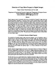
Figure 1. Shown are: (a) the investigated region b(x, y) (denoted by a black box, 256 × 256 pixels); the output of the resampling detection method using Dr2 {b(x, y)} (figure b); Dr5 {b(x, y)} (figure c) and Dr9 {b(x, y)} (figure d). Peaks belong to the resizing operation. The investigated image was resized by factor 1.9 using the bicubic interpolation.

Figure 2. Shown are: (a) the investigated region b(x, y) (denoted by a black box, 256 × 256 pixels); the output of the resampling detection method using Dr2 {b(x, y)} (figure b); Dr5 {b(x, y)} (figure c) and Dr9 {b(x, y)} (figure d). In (d) both resizing and rotation peaks are detected. The investigated image was rotated by angle 9◦ and then resized by factor 1.9 using the bicubic interpolation.

7. EXPERIMENTAL RESULTS Figures 1 and 2 show outputs of the method applied to a uncompressed image that have undergone various transformations. Shown are the outcomes based on rows derivatives. The size of the investigated region (denoted by a black box) in all cases is 256 × 256 pixels. It is apparent that peaks signifying interpolation are clearly detectable. Figure 2 shows the advantages of using various derivative filters. As shown, derivative of order 9 allowed to also detect the rotation transformation, which has been applied to the image before a dominant resizing operation (resizing factor 1.9).

Figure 3. Shown are the original image (a), the doctored image containing a forged resized region additionally corrupted by local additive white Gaussian noise with σ = 5(b), output of the resampling detection method (due to noise it failed) (c) and output of the noise inconsistencies detection method applied to the doctored image (b).

In the second part of this section, a quantitative measure of the efficiency of the proposed interpolation detection method is carried out. The method has been applied to 20 images corrupted by various transformations. The size of test images was 256 × 256 pixels. In all cases the bicubic interpolation method was used. The method was applied separately to rows and columns of tested images. All experiments were carried out in Matlab. Table 1 shows the detection accuracy of the method applied to uncompressed resized images. The detection accuracy expresses the success of the method in expressing the present geometric transformations by clear and easily detectable peaks, either in row–based or column–based output obtained from any of derivative signals. Table 2 shows the detection accuracy of the proposed method applied to rotated images. Table 3 shows the detection accuracy of the method for affine transformation (resizing followed by rotation). Here, the detection accuracy expresses the success of the method in detecting both present geometric transformations. Noisy images were obtained by adding white gaussian noise to the transformed images. During the experimental phase, the method was also applied to the original (non–interpolated) versions of tested images. This resulted in a false positive rate of 10%. For correctly detected resized images, we tried also to estimate the particular scaling factors using the position of the occurred corresponding peaks. This was carried out for scaling factors greater than 1.05 shown in Table 1. The estimation accuracy was near 100%. The same was carried out for rotated TIFF format images (for rotation angles greater than 5◦ shown in Table 2). Also here, based on the interpolation peaks positions, we tried to estimate the particular rotation angles. The detection accuracy was again near 100%. A quantitative measure of the efficiency of the noise estimation method was also carried out. Experimental results are obtained by applying the estimator to 20 non–compressed test images corrupted by additive Gaussian noise with various standard deviations. Here, the size of test images was 512 × 512 pixels. These images were tiled by non–overlapping blocks of various sizes. The method was applied to each block separately. In other

512 words, each analyzed noise standard deviation corresponds to 20 × b 512 R c × b R c estimations, where R is the ¯ˆ ), block’s size. Obtained results are shown in Table 4 and Table 5 in terms of mean value of σ estimation (σ ¯ average error (E) and its standard deviation (σE ), maximum and minimum obtained absolute errors (maxEi and minEi ). Statistics were obtained as a function of different noise standard deviations σ = 0 (noise–free image), 2, 3, 5, 7, 10, 15, 20 and 25.

Table 1. Detection accuracy [%] as a function of different scaling factors. Each cell corresponds to the average detection accuracy from 20 images.

scaling factor TIFF SNR 30 dB

1.05 100 95

1.10 100 100

1.20 100 100

1.30 100 100

1.40 100 100

1.50 100 100

1.60 100 100

1.70 100 100

1.80 100 100

1.90 100 100

Table 2. Detection accuracy [%] as a function of different rotation angles. Each cell corresponds to the average detection accuracy from 20 images.

rotation angle TIFF SNR 30 dB

5◦ 100 95

10◦ 100 100

15◦ 100 100

20◦ 100 100

30◦ 100 90

40◦ 100 90

Table 3. Detection accuracy [%] for resizing followed by rotation. Each cell corresponds to the average detection accuracy from 20 images.

5◦ 10◦ 20◦ 30◦ 40◦

1.05 100 95 45 95 100

1.10 100 100 100 95 100

1.15 100 100 95 100 95

1.20 100 90 85 95 90

1.25 95 100 90 90 90

1.30 90 95 90 90 90

1.35 85 90 95 80 85

1.40 85 90 90 90 90

1.45 95 95 90 85 90

¯ σE , max(Ei ) and min(Ei ) as Table 4. Shown are the statistics of estimated noise standard deviations mean(ˆ σ ), E, functions of different σ. These statistics have been obtained by analyzing 2880 non–overlapping blocks of size 40 × 40 from 20 images of size 512 × 512. TIFF ¯ ¯ σ σ ˆ E σE maxEi minEi 0 1.90 1.90 1.10 9.70 0.00 2 3.00 0.99 0.80 7.40 0.00 3 3.80 0.82 0.69 6.90 0.00 5 5.50 0.66 0.57 5.70 0.00 10 10.00 0.70 0.66 4.70 0.00 15 15.00 0.93 0.97 6.90 0.00 20 20.00 1.30 1.40 10.00 0.00 25 24.00 1.70 1.80 13.00 0.00 ¯ σE , max(Ei ) and min(Ei ) as Table 5. Shown are the statistics of estimated noise standard deviations mean(ˆ σ ), E, functions of different σ. These statistics have been obtained by analyzing 1280 non–overlapping blocks of size 64 × 64 from 20 images of size 512 × 512. TIFF ¯ ¯ σ σ ˆ E σE maxEi minEi 0 1.80 1.80 1.00 5.50 0.00 2 3.00 0.96 0.72 4.10 0.00 3 3.80 0.79 0.61 3.60 0.00 5 5.50 0.61 0.48 3.10 0.00 10 10.00 0.55 0.57 4.30 0.00 15 15.00 0.70 0.88 6.60 0.00 20 20.00 0.95 1.30 9.50 0.00 25 24.00 1.30 1.70 11.00 0.00

8. DISCUSSION In this paper we extended our previous work.14 In that work, our aim was to detect whether the image being investigated contains any traces of interpolation. Here, our goal was to analyze whether the presented method can be helpful in detecting all geometrical transformations present in the image. Experiments showed that by using a combination of filters, traces of most geometrical transformations present in the image can be found and the position of their corresponding peaks used to easily determine the scaling factors or rotation angles. A weakness of this approach is that some transformations have indistinguishable periodic patterns in the output of the method. The main advantage of the method is that it makes possible in a simple and fast way find traces of general affine transformation. The proposed method works well for low order interpolation polynomials: nearest neighbor, linear or cubic. The detection performance decreases as the order of interpolation polynomial increases. Different interpolation orders introduce correlations of varying degrees between neighboring samples. These correlations become more difficult to detect as each interpolated sample value is obtained as a function of more samples. Furthermore, like other existing methods, our approach has weak results when the interpolated images is altered by further operations like noise addition, linear or median filtering. These operations make the interpolation–based pixels correlation corrupted and difficult to detect. By applying the method to JPEG compressed images, the detection performance decreases. JPEG is a lossy compression format. It brings noise into the image. Experiments show that the presented method works well for JPEG compression quality of 95 - 100. But, generally, the results obtained are based on image properties. Obtained results of the noise inconsistencies detection part show that the proposed method makes it possible in a simple and blind way to divide an investigated image into various segments with homogenous noise level. The main weakness of the noise inconsistencies detection method is that authentic images also can contain various isolated regions with totally different variances (non–stationarity). Therefore the method is more appropriate as a supplement to other forgery detection methods than a stand alone detector. Typically, this method is not able to find the corrupted regions, when the noise degradation is very small (σ < 2). However, please note that this is not a significant limitation. When the method is used as a supplement to resampling detector, in the case of minor noise degradation, the resampling detector does not fail. In this work we have been concerned with gray-level images. There are several ways to adopt the presented methods for RGB images. For instance, the method can be applied to each channel separately.

ACKNOWLEDGMENTS This work has been supported by the Czech Science Foundation under the project No. GACR 102/08/0470.

REFERENCES [1] Sencar, H. T., Ramkumar, M., and Akansu, A. N., [Data Hiding Fundamentals and Applications: Content Security in Digital Multimedia ], Academic Press, Inc., Orlando, FL, USA (2004). [2] Wu, M. and Liu, B., [Multimedia Data Hiding ], Springer-Verlag New York, Inc., Secaucus, NJ, USA (2002). [3] Schneider, M. and Chang, S. F., “A robust content based digital signature for image authentication,” in [IEEE International Conference on Image Processing (ICIP’96) ], (1996). [4] Lu, C. S. and Liao, H. M., “Structural digital signature for image authentication: an incidental distortion resistant scheme,” in [MULTIMEDIA ’00: Proceedings of the 2000 ACM workshops on Multimedia], 115– 118, ACM Press, New York, NY, USA (2000). [5] Lin, C. Y. and Chang, S. F., “Generating robust digital singnature for image/video authentication,” in [ACM Multimedia Workshop ], 115–118 (1998). [6] Popescu, A. and Farid, H., “Exposing digital forgeries in color filter array interpolated images,” IEEE Transactions on Signal Processing 53(10), 3948–3959 (2005). [7] Lukas, J., Fridrich, J., and Goljan, M., “Digital camera identification from sensor pattern noise,” IEEE Transactions on Information Forensics and Security 1, 205–214 (June 2006).

[8] Dehnie, S., Sencar, H. T., and Memon, N. D., “Digital image forensics for identifying computer generated and digital camera images,” in [ICIP], 2313–2316, IEEE (2006). [9] Mahdian, B. and Saic, S., “Detection of copy–move forgery using a method based on blur moment invariants,” Forensic science international 171(2–3), 180–189 (2007). [10] Sutcu, Y., Coskun, B., Sencar, H. T., and Memon, N., “Tamper detection based on regularity of wavelet transform coefficients,” in [ICIP: IEEE International Conference on image Processing ], 397–400, IEEE (2007). [11] Meijering, E., “A chronology of interpolation: From ancient astronomy to modern signal and image processing,” Proceedings of the IEEE 90, 319–342 (March 2002). [12] Parker, J. A., Kenyon, R. V., and Troxel, D. E., “Comparison of interpolation methods for image resampling,” IEEE Transactions on Medical Imaging 2(1), 31–39 (1983). [13] Hou, H. and Andrews, H., “Cubic splines for image interpolation and digital filtering,” IEEE Transactions on Acoustics, Speech and Signal Processing 26(6), 508–517 (1978). [14] Mahdian, B. and Saic, S., “Blind authentication using periodic properties of interpolation,” IEEE Transactions on Information Forensics and Security 3, 529–538 (September 2008). [15] Popescu, A. and Farid, H., “Exposing digital forgeries by detecting traces of re-sampling,” IEEE Transactions on Signal Processing 53(2), 758–767 (2005). [16] Bayram, S., Avcibas, I., Sankur, B., and Memon, N., “Image manipulation detection,” Journal of Electronic Imaging 15, 041102–1 – 041102–17 (December 2006). [17] Kirchner, M., “Fast and reliable resampling detection by spectral analysis of fixed linear predictor residue,” in [Proceedings of the 10th ACM workshop on Multimedia and security], 11–20, ACM, New York, NY, USA (2008). [18] Prasad, S. and Ramakrishnan, K. R., “On resampling detection and its application to image tampering,” in [Proceedings of the IEEE International Conference on Multimedia and Exposition], 1325–1328 (2006). [19] Rohde, G., Berenstein, C., and Healy, D., “Measuring image similarity in the presence of noise,” Proceedings of the SPIE Medical Imaging: Image Processing 5747, 132–143 (February 2005). [20] Zlokolica, V., [Advanced Nonlinear Methods for Video Denoising ], Ph.D. Thesis, Ghent University, Gent, Belgium (2006). [21] Stefano, A. D., White, P. R., and Collis, W. B., “Training methods for image noise level estimation on wavelet components,” EURASIP J. Appl. Signal Process. 2004(1), 2400–2407 (2004).