822
JOURNAL OF NETWORKS, VOL. 8, NO. 4, APRIL 2013
Detection and Recovery of Coverage Holes in Wireless Sensor Networks Zhiping Kang Key Laboratory of Optoelectronic Technology and System of Ministry of Education, Chongqing University, Chongqing, China Email:
[email protected]
Honglin Yu1 and Qingyu Xiong 2 1 Key Laboratory of Optoelectronic Technology and System of Ministry of Education, Chongqing University, Chongqing, China 2 School of Software Engineering, Chongqing University, Chongqing, China Email:
[email protected],
[email protected]
Abstract—Wireless Sensor Networks (WSN) consists of distributed low-cost sensing nodes with autonomous network. Several anomalies can occur in wireless sensor networks that may form various coverage holes. These holes may disturb the existing coverage or connectivity, and impair desired functionalities of networks. Hence, it is essential to detect and recovery coverage holes in order to ensure the full operability of a WSN. In the paper, we propose a decentralized, coordinate-free, node-based coverage hole detection algorithm. It is based on boundary critical points, and can be run on a single node with verifying boundary critical points from neighbors. The hole patching algorithm is implemented with the concept of perpendicular bisector and our detection algorithm. The patching sensor nodes are deployed on hole boundary bisectors. Simulation demonstrates that our algorithm can detect and recover coverage hole, and guarantee full coverage in hostile environments with an effective manner. Index Terms—wireless sensor networks, coverage problem, detecting holes, patching holes
I. INTRODUCTION Wireless Sensor Network (WSN) is autonomous distributed network, which has spread rapidly into various potential applications such as military security[1,2], environmental protect[3,4], industrial process monitoring[5,6] , agriculture and farming [7], structural health monitoring[8-10] , passive localization or tracking[11] and so on. Many of these applications require a reliable connectivity and coverage, which can be guaranteed only if the target field monitored by a WSN contains no coverage holes. Coverage holes can be formed for many reasons, such as intrusion, explosion, environmental factors, software bugs and energy depletions [12, 13].These holes result in no uniform sensor deployments, and impair their functionality, or shorten the lifetime[14].Consequently, it is essential to Corresponding author: Zhiping Kang
© 2013 ACADEMY PUBLISHER doi:10.4304/jnw.8.4.822-828
detect and recovery coverage holes in order to ensure the full operability of a WSN. There is already an extensive literature about the coverage hole problems in WSNs. S. Ganeriwal, A. Kansal, et al. [15] adopt self-aware actuation for coverage maintenance in sensor networks, and present Coverage Fidelity maintenance algorithm (CO-Fi). They utilize the mobility of nodes to repair the coverage loss of the area. The dying node requests for updating the network topology, sensing neighbors of the dying node responds to request message only if it can move without losing coverage, then the dying node decides which optimization node to move. Authors of [16] Wang et al. presented the Coverage Configuration Protocol (CCP) that can provide flexibility in configuration of sensor network to self-configure for different degrees of coverage. Heo et al. [17] proposed two schemes for addressing single coverage problem. In one scheme called Distributed Self-Spreading Algorithm (DSSA), which is inspired by minimizing molecular electronic energy and inter-nuclear repulsion in equilibrium of molecules. Another scheme called Intelligent Deployment and Clustering Algorithm (IDCA), which utilize low energy consumption characteristics of local clustering. W. Guiling, et al. [18] used Voronoi diagrams to discover the coverage holes, movement-assisted sensor to eliminate or reduce the size of hole. The proposed deployment protocols are VEC (VECtorbased),VOR (VORonoi-based), and Minimax, which based on the principle of moving sensors from densely deployed areas to sparsely deployed areas Fang et al.[19] detected the hole boundaries by a distributed algorithm to enable the formation of new routes. It is useful for route formation, but does not offer a solution for mitigating the hole problem. Li and David K. Hunter [20] proposed a Triangular Mesh Self-organizing self-Healing protocol (3MeSH) for full sensing coverage, which conserve energy by electing as few active nodes as possible. But the algorithm only account every sensor node has a uniform sensing disk of
JOURNAL OF NETWORKS, VOL. 8, NO. 4, APRIL 2013
radius R, with the first hop being within a radio transmission range of 3R . Robert et al.[21] introduced means of homology for detecting holes in coverage, and give two objects: Cech complex, Rips complex from simplicial complexes based on its communication graph. The Cech complex can fully characterizes coverage properties of a WSN, but is very difficult to compute. The Rips complex is easy to construct by simple algebraic calculations, but does not in itself yield coverage data, and is at the expense of accuracy. Feng Yan et al.[22] took emphasis on Rips complex to solve triangular holes. They evaluate accuracy for triangular holes, under different ratios between communication radius and sensing radius of each sensor. Jinko Kanno et al.[23] simplified homology and counting holes, then take to locate holes by a divide-andconquer strategy. J Yao, G Zhang et al.[24] presented sensor network coverage hole detection and patching using modeling by simplicial complexes. The hole-patching algorithm (HPA) is based on perpendicular bisector, and is dependent on previous hole detection methods. The algorithm is efficient and useful even if only partial sensor node coordinate information is available. However, it might add redundant nodes, and is not optimal in terms of the number of patching nodes. Prasan Kumar Sahoo et al.[25] designed distributed coverage hole recovery algorithms, which use the vector methods decide the magnitude and direction of a mobile node, and guarantee highest coverage of a node is not increased. But the mobility is limited within only one hop; it still exist fragment of holes. As alluded above, some researchers have proposed connectivity and coverage maintenance algorithms, but a majority of them using a complicated network model, or only providing partial coverage for patching. Some current algorithms are centralized which will become extremely time consuming, as the number of sensor nodes becomes significantly large. In this paper, we propose the distributed coverage hole detection and recovery algorithms, and guarantee full coverage in hostile environments with an effective manner. The main contribution of our work can be summarized as follows. (1) We introduce a concept of boundary critical points (BCPs), not maximal simplicial complex or Voronoi Diagram for detecting. (2) We bring forward a decentralized, coordinate-free, node-based coverage hole detection algorithm without knowing exact locations of nodes. (3) Our proposed patching algorithm is based on the concept of perpendicular bisector and BCPs, which provide full coverage, not proportion. The remainder of the paper is organized as follows. Problem formulations with few definitions related to our work are given in Section II. Our detection and recovery algorithms are described in Section III. Performance analyses are presented in Section IV. The conclusion and future work are made in Section V. II. PROBLEM FORMULATION
© 2013 ACADEMY PUBLISHER
823
A. Network Model It is considered that the sensors are distributed randomly over a large target region A , and designed to detect specified events. Each every one of sensors can sense specified events in its sensing range, and communicate with others in its transmission range. For the sake of simplicity, we assume that sensing and transmission ranges of a node S are disks with radiuses Rs and Rt , accordingly, where Rt ≥ 2 Rs , and there are no two sensors at the same location, each sensor has a unique ID. Given a set of sensors and a target area, no coverage hole exists in the target area, if every point in that target area is covered by at least k sensors, where k is the required degree of coverage for a particular application [26].A point p is covered by a node S if their Euclidian distance is less than the sensing range of S , Rs , i.e., p, s < Rs . Based on the above coverage model, we define a region A (that contains convex or non-convex region) as having a coverage degree of k (i.e., being k -covered) if every location inside A is covered by at least k nodes. Practically speaking, a network with a higher degree of coverage can achieve higher sensing accuracy and be more robust against sensing failures. B. Definitions Definition 1: Sensing Circle We define the sensing circle C ( S ) of node S as the boundary of S ’s coverage region. For simplifying our geometric analysis, we assume that any point p on the sensing circle C ( S ) (i.e., pS = Rs ) is not covered by S , which has an insignificant practical impact. Definition 2: Sensing Neighbors The sensing neighbors of node S are denoted N s ( S ) , which includes all the nodes that are within a distance of twice the sensing range, i.e.
= N s (S )
{S : i
S i S < 2 Rs
}
Definition 3: Intersection Points The point p lies only on the sensing circle of Si and S j or on the boundary of the monitoring region. At least it meets the following conditions: (1) It lies on the intersection of two nodes , i.e. = pSi = pS j Rs . (2) It lies on the sensing circle of S and the boundary of the target region A . Definition 4: Boundary Critical Point (BCP) The intersection points of node S with its sensing neighbors, which can’t be covered by other k nodes. k is above-mentioned coverage degree.( e.g. k = 1 ,the boundary critical point bi is one of intersection points, and is not covered by any node.) Definition 5: Boundary Line The connecting consecutive boundary critical points can form boundary line. Definition 6: Coverage Hole
824
JOURNAL OF NETWORKS, VOL. 8, NO. 4, APRIL 2013
The area H can’t be covered by any node in the target region A , which is surrounded by joining the consecutive boundary critical points, and constitute of consecutive boundary lines. It can be classified into Close Hole and Open Hole. Close Hole: It is completely enclosed by boundary lines. Open Hole: It is enclosed by boundary lines and the boundary of target region.
A. Boundary Critical Point Detecingt As discussed in the previous section, the sensors that are not along the boundary of any coverage holes cannot have any boundary critical point. We design here an algorithm to detect boundary critical points of each sensor. The detail procedure is given in Table I. TABLE I BOUNDARY CRITICAL POINT DETECTING Step 1: Choose a sensor node S from network, and obtain its sensing neighbor set N s ( S )
.
Step2: Create a list of sensing neighbors of S by sorting them in clockwise. Step3: Create a list for intersection points ( pi ) : (1) node S and each of its sorted sensing neighbors; (2) node S and the boundary of the monitoring region; Step4: Verify if each point of list ( pi
) is a boundary critical point
( bi ) or not, and remove the non-boundary critical points; Step5:Update the list of boundary critical points ( bi )in clockwise; Step 6: Continue this procedure for all nodes of the network. Figure 1. Example of intersection points, boundary critical points and coverage holes.
As shown in Figure 1, when coverage degree k = 1 , S9 , S 2 are the sensing neighbor of S1 , since the distance of ( S1 , S9 ) , ( S1 , S 2 ) are less than twice the sensing range. The intersection points of nodes S1 and S 2 are p1 , p4 . Similarly, the intersection points of S1 and S9 are p3 , p6 ,
S1 and target region are p2 , p5 . S1 has no boundary critical points, since all of its intersection points either lies outside of the monitoring region or within sensing disc of another sensing neighbor. b1 is a boundary critical point of S 2 , since b1 is a intersection point of S 2 and S9 ,and lies on the sensing disc of S 2 , S9 , not covered by any sensor node. Similarly, b2 to b14 are belong to boundary critical points, and they are not covered by any node. Correspondingly, the line b1b2 , b2 b3 , b3b4 , b5b6 , b6 b7 , b7 b8 , b8b1 , b9 b10 , b10 b11 ,
b11b12 , b12 b13 , b13b14 are boundary lines. Obviously,
Lemma 1: Any two adjacent points in the list of boundary critical points, bi and b j , i, j > 0 , then
| bi , b j |≤ 2 Rs Proof: From the constructing of boundary critical points’ list, any two adjacent points bi , b j lie on the same sensor circle. It shows that the Euclidian distance of those is not more than twice of the sensing range Rs . The LEMMA 1 implies that a sensor with radiuses Rs can cover both of two adjacent points. It will be useful for patching holes. B. Hole Detecting based on BCPs It is to be noted that the sensors which enclose any close or open hole can have boundary lines. We design HDBCP by constructing the boundary lines. The detail procedure is given in Table II. TABLE II PSEUDO HOLE DETECTING BASED ON BCPS
boundary lines b1b2 to b8b1 may form a closed area,
Step 1: Run Boundary Critical Point Detecting Algorithm; Step2: Connect each consecutive boundary critical points ( bi ) by
which is close hole H1 .Lines from b9 b10 to b13b14 form a open hole H 2 .
constructing an boundary line along the border of the nodes having bi ;
III. DETECTION AND RECOVERY ALGORITHM In this section, we describe Hole Detection based Boundary Critical Points (HDBCP), Hole Patching based Boundary Critical Points (HPBCP) for detecting and patching hole, respectively. Both of them based on boundary critical points, one is how to find the points; the other one is how to eliminate. Perpendicular bisector is used to find positions (exact coordinates are not required) of new nodes for hole patching.
© 2013 ACADEMY PUBLISHER
Step 3: Continue the construction of boundary line till the starting boundary critical point bi is revisited, or border of the monitoring region is touched; Step 4: Continue this procedure for all nodes of the network.
C. Removing Redundant BCPs The goal of this part is to reduce redundant BCPs for Location Calculation Algorithm, so that the hole is patched with minimum new sensor nodes. An example of removing BCP algorithm is shown in Figure 2.
JOURNAL OF NETWORKS, VOL. 8, NO. 4, APRIL 2013
825
(a)
(b)
Figure 2. Example of Remove redundant BCPs
Figure 3. Location for new nodes: Two adjacent critical points (a); Multi-adjacent critical points (b)
Let b1 , b2 , …, b7 are boundary critical points from a hole. According Lemma 1, a node may cover two adjacent boundary critical points. As for b1 , b2 , we can
The location calculation is classified two modes: (1) two adjacent critical points: Find a position N on the bisector of bi bi +1 such that Nbi and Nbi +1 are
find a position N1 on the bisector of b1b2 such that N1b1 and N1b2 are approximately equal to sensor radius
approximately equal to sensing radiuses R0 ; (2) multiadjacent critical points: Find a position N on the bisector of line from beginning point to end point, such that the maximal Nb j is approximately equal to R0 . The detail
Rs . After the new node locates on position N1 , the points b1 , b2 and their corresponding areas will be covered. Similarly, a position N 2 can be located on the bisector of b2 b3 . From Figure 2, the two new nodes in position N1 and N 2 include large of common areas, which affects the coverage degree of new nodes. Under certain conditions, we may don’t consider b2 , and obtain position N 3 on the bisector of b1b3 ,which can replace position N1 and N 2 .The detail procedure of above discussion is given in Table Ⅲ. In order to satisfy the definition 1, we adopts R0 instead of Rs , which is approximate to sensing radiuses Rs , R0 =Rs − σ , σ is a accepted tiny value.
procedure of algorithm is given in Table Ⅳ. TABLE Ⅳ PSEUDO LOCATION CALCULATION FOR NEW NODE Step 1: Input a point bi from boundary critical point list, and run Remove BCP Algorithm; Step 2: Obtain critical points bi and b j ; Step3: IF bi
and b j are two adjacent critical points:
Find a position N on the bisector of bi b j such that Nbi and Nb j are approximately equal to R0 ;
Else Find a position N on the bisector of bi b j , such that the maximal Nbk is approximately equal to R0 , i < k < j ;
TABLE III PSEUDO REMOVE REDUNDANT BCPS
Step4: Add a patching node on the position N.
Step 1: Input a point bi from boundary critical point list; Step 2: Select the next adjacent point b j in clockwise, j=i+2, flag=false; Step 3: Calculate Euclidian distance from bi to b j ; Step 4: When it satisfies the followings condition: (1) bi , b j ≤ 2 R0 ; (2) It can find a point N 0 on the bisector of bi b j
,
N 0 , bk ≤ R0 , i < k < j .
Then j=j+1 and flag=true, go back Step3 till the all points of the list is visited. Else go to Step5 Step 5: if flag==true, then return j Else return j=j-1.
D. Location Calculation for new nodes After reducing some redundant boundary critical points, we calculate location for new deployed nodes on the bisectors of boundary lines. An example is shown in Figure 3.
© 2013 ACADEMY PUBLISHER
E. Hole Patching based on BCPs The above discussion is not enough; we introduce following rule to maximize coverage for each adding new sensor node. Lemma 2: The priority selected the shortest two adjacent points from boundary critical lists. It is obviously that the rule ensure the new node coverage maximize hole areas. Above all, the whole Hole Patching can be described in Table V. TABLE V PSEUDO OUR HOLE PATCHING ALGORITHM Step 1: Run the Boundary Critical Point Detecting Algorithm to get the boundary critical point list; Step 2: Selected a point bi , which owns the shortest distance to its adjacent point from boundary critical lists; Step 3: Run Remove BCP Algorithm, and get bi and b j ; Step4: Run Location Calculation Algorithm, and deploying a new node on the position N; Step5: Continue this procedure until the boundary critical point list is NULL.
826
JOURNAL OF NETWORKS, VOL. 8, NO. 4, APRIL 2013
F. Discussion It is to be noted that each node determines its boundary critical point from its one-hop neighbor without other information. Hence, the algorithm is distributed, coordinate-free. The algorithm runtime or complexity depends on several factors in the network including the number of nodes, number of holes, and size of the holes. Consider the algorithm in Table Ⅴ, let d be the maximum number of sensors that are neighboring to a sensor (d≤ n). The variable m is the maximum number of BCPs in the network (m≤n). The complexity of Step1 is O (dn). From Step2 to Step4, complexities of them are O (2m). The calculation of Step5 takes time O(m), the overall complexity is O(mdn). When sensor nodes coordinates are known, hole patching is more efficient and requires less computation. The performance evaluations of our algorithms are analyzed in section IV.
S is the whole area of coverage hole, and Si is the coverage area by patching nodes. From definition, Re reflects recovery degree of new nodes. When we add 50 nodes, the 2.544% of polygon area is covered by nodes. After 500 nodes are used, the recovery degree will achieve 96%.More experiment data are shown in Table VI.
IV. PERFROMANCE EVALUATION
The fitting curve is given as Figure 5, which show an approximate linear relation between recovery degree and deployed nodes. It implies that the algorithm has better convergence. With the increase of sensor nodes, recovery degree is nearly linear growth, indicating that each node can reduce areas of coverage hole
A. Simulation Setup Our algorithms are simulated using MatLab 7.0 for different number of nodes that are deployed randomly over 100m × 100m. The number of deployed nodes varies from 100 to 200. For each sensor node, the sensing range is 10m, and communication range is twice of the sensing range 20m. The network is homogenous, and coverage degree k = 1 . We use polygon simulating different coverage holes. The simulation results are averaged over 20 independent runs. B. Simulation Result Experiment I: Patching of Randomly Deployed WSNs We randomly deployed 100 sensor nodes and created coverage holes, see Figure 4. Simulations show that our algorithm works well when more than one hole exist in a randomly deployed network, even when some holes are open holes or non-convex holes. One can see that our successfully patched the network with 100 initial nodes.
(a)
(b)
Figure 4. Randomly deployed WSN with initial 100 sensors and three separate holes exist (a); no hole left after patching (b).
TABLE VI EXPERIMENT II RECOVERY CONFIGURATION Recovery Degree(%) Number of Sensors Recovery Degree(%) Number of Sensors
2.544
7.875
15.856
25.985
37.627
50.049
50
100
150
200
250
300
62.472
74.113
84.243
96.00
100
/
350
400
450
500
518
/
Figure 5. The relationship between deployed nodes and recovery degree.
Experiment III: Comparing with HPA HPA is based on the concept of perpendicular bisector line [24]. Every hole boundary edge has a corresponding perpendicular bisector and patching nodes are deployed on hole-boundary bisectors. In order to compare with HPA, we randomly deployed 30 sensor nodes in an area 100m*70m form a coverage hole. Then run two algorithms independently to patch the coverage hole.
Experiment Ⅱ: Coverage analysis We choose a 100-regular polygon as a coverage hole, and length of edge is 10m. We use algorithms to recover the regular polygon. It is performed on the recovery degree by the following formula:
Re =
( S ) S i
© 2013 ACADEMY PUBLISHER
i
S
(1) (a)
(b)
JOURNAL OF NETWORKS, VOL. 8, NO. 4, APRIL 2013
827
REFERENCES
(c)
(d)
Figure 6. Simulation of network environment using HPA and our algorithm: HPA with simulation 1 (a), HPBCP with simulation 1 (b); HPA with simulation 2 (c), HPBCP with simulation 2 (d).
As shown in Figure 6, instance (a) and (b) give a same coverage hole, both of HPA and our algorithms adopts 13 new sensors to patch. In (c) and (d), HPA needs 16 sensors, our algorithm require 17 sensors. To all appearances, our algorithm is equal or more HPA for number of patching nodes. But we provide a full coverage; HPA brings many fragment of hole. If HPA also achieve full coverage, the number of sensors will much higher than the algorithm. As shown in Figure 7, we record the experiment for 20 independent runs, and obtain number of sensors by patching with HPA, HPBCP.
Figure 7. The comparing with HPA and HPBCP for patching
V. CONCLUSION AND FUTURE WORK The paper proposes a solution for distributed coverage hole detection (HDBCP) and patching (HPBCP) in coordinate-free wireless sensor networks, which based on perpendicular bisector and boundary critical points. Simulation results show successful hole detection and patching in case of both grid-type networks and randomly deployed networks. The evaluation only shows the algorithms single coverage based, but also can run in highest coverage (k-coverage). The algorithm is efficient and useful even if only partial sensor node coordinate information is available. Further research and simulation will use our proposed algorithms in reality, and also focus on an optimal process to reduce the complexity of the algorithm. ACKNOWLEDGMENT This work was financially supported by the National Natural Science Foundation of China (50975300) and Higher School Specialized Research Fund for the Doctoral Program (20100191110038).
© 2013 ACADEMY PUBLISHER
[1] G. Simon, M. Maróti, Á. Lédeczi, G. Balogh, B. Kusy, A. Nádas, et al., "Sensor network-based countersniper system," in Proceedings of the 2nd international conference on Embedded networked sensor systems, 2004, pp. 1-12. [2] T. Bokareva, W. Hu, S. Kanhere, B. Ristic, N. Gordon, T. Bessell, et al., "Wireless sensor networks for battlefield surveillance," in Proceedings of the land warfare conference, 2006. [3] Y. Ma, M. Richards, M. Ghanem, Y. Guo, and J. Hassard, "Air pollution monitoring and mining based on sensor grid in London," Sensors, vol. 8, pp. 3601-3623, 2008. [4] J. D. Kenney, D. R. Poole, G. C. Willden, B. A. Abbott, A. P. Morris, R. N. McGinnis, et al., "Precise positioning with wireless sensor nodes: Monitoring natural hazards in all terrains," in Systems, Man and Cybernetics, 2009. SMC 2009. IEEE International Conference on, 2009, pp. 722727. [5] V. C. Gungor and G. P. Hancke, "Industrial wireless sensor networks: Challenges, design principles, and technical approaches," Industrial Electronics, IEEE Transactions on, vol. 56, pp. 4258-4265, 2009. [6] K. S. Low, W. N. N. Win, and M. J. Er, "Wireless sensor networks for industrial environments," in Computational Intelligence for Modelling, Control and Automation, 2005 and International Conference on Intelligent Agents, Web Technologies and Internet Commerce, International Conference on, 2005, pp. 271-276. [7] K. Shinghal, A. Noor, N. Srivastava, and R. Singh, "Wireless Sensor Networks in Agriculture: for potato farming," International Journal of Engineering Science and Technology, vol. 2, pp. 3955-3963, 2010. [8] A. Basharat, N. Catbas, and M. Shah, "A framework for intelligent sensor network with video camera for structural health monitoring of bridges," in Pervasive Computing and Communications Workshops, 2005. PerCom 2005 Workshops. Third IEEE International Conference on, 2005, pp. 385-389. [9] S. Kim, S. Pakzad, D. Culler, J. Demmel, G. Fenves, S. Glaser, et al., "Wireless sensor networks for structural health monitoring," in Proceedings of the 4th international conference on Embedded networked sensor systems, 2006, pp. 427-428. [10] S. Kim, S. Pakzad, D. Culler, J. Demmel, G. Fenves, S. Glaser, et al., "Health monitoring of civil infrastructures using wireless sensor networks," in Information Processing in Sensor Networks, 2007. IPSN 2007. 6th International Symposium on, 2007, pp. 254-263. [11] F. Viani, P. Rocca, M. Benedetti, G. Oliveri, and A. Massa, "Electromagnetic passive localization and tracking of moving targets in a WSN-infrastructured environment," Inverse Problems, vol. 26, p. 074003, 2010. [12] L. Frye, L. Cheng, S. Du, and M. W. Bigrigg, "Topology maintenance of wireless sensor networks in node failureprone environments," in Networking, Sensing and Control, 2006. ICNSC'06. Proceedings of the 2006 IEEE International Conference on, 2006, pp. 886-891. [13] H. Ng, M. Sim, and C. Tan, "Security issues of wireless sensor networks in healthcare applications," BT Technology Journal, vol. 24, pp. 138-144, 2006. [14] N. Ahmed, S. S. Kanhere, and S. Jha, "The holes problem in wireless sensor networks: a survey," ACM SIGMOBILE Mobile Computing and Communications Review, vol. 9, pp. 4-18, 2005. [15] S. Ganeriwal, A. Kansal, and M. B. Srivastava, "Self aware actuation for fault repair in sensor networks," in Robotics
828
[16]
[17]
[18]
[19]
[20]
[21]
[22]
[23]
JOURNAL OF NETWORKS, VOL. 8, NO. 4, APRIL 2013
and Automation, 2004. Proceedings. ICRA '04. 2004 IEEE International Conference on, 2004, pp. 5244-5249 Vol.5. X. Wang, G. Xing, Y. Zhang, C. Lu, R. Pless, and C. Gill, "Integrated coverage and connectivity configuration in wireless sensor networks," in Proceedings of the 1st international conference on Embedded networked sensor systems, 2003, pp. 28-39. H. Nojeong and P. K. Varshney, "An intelligent deployment and clustering algorithm for a distributed mobile sensor network," in Systems, Man and Cybernetics, 2003. IEEE International Conference on, 2003, pp. 45764581 vol.5. W. Guiling, C. Guohong, and T. La Porta, "Movementassisted sensor deployment," in INFOCOM 2004. Twentythird Annual Joint Conference of the IEEE Computer and Communications Societies, 2004, pp. 2469-2479 vol.4. F. Qing, G. Jie, and L. J. Guibas, "Locating and bypassing routing holes in sensor networks," in INFOCOM 2004. Twenty-third Annual Joint Conference of the IEEE Computer and Communications Societies, 2004, pp. 24582468 vol.4. X. Li and D. K. Hunter, "3MeSH for full sensing coverage in a WSN without location awareness," in London Communications Symposium, 2005. R. Ghrist and A. Muhammad, "Coverage and holedetection in sensor networks via homology," in Information Processing in Sensor Networks, 2005. IPSN 2005. Fourth International Symposium on, 2005, pp. 254260. F. Yan, P. Martins, and L. Decreusefond, "Accuracy of homology based approaches for coverage hole detection in wireless sensor networks," in Communications (ICC), 2012 IEEE International Conference on, 2012, pp. 497-502. J. Kanno, J. G. Buchart, R. R. Selmic, and V. Phoha, "Detecting coverage holes in wireless sensor networks," in Control and Automation, 2009. MED'09. 17th Mediterranean Conference on, 2009, pp. 452-457.
© 2013 ACADEMY PUBLISHER
[24] J. Yao, G. Zhang, J. Kanno, and R. Selmic, "Decentralized detection and patching of coverage holes in wireless sensor networks," in Proc. of SPIE, 2009, p. 73520V. [25] P. K. Sahoo, T. Jang-Zern, and K. Hong-Lin, "Vector method based coverage hole recovery in Wireless Sensor Networks," in Communication Systems and Networks (COMSNETS), 2010 Second International Conference on, 2010, pp. 1-9. [26] C. F. Huang and Y. C. Tseng, "The coverage problem in a wireless sensor network," Mobile Networks and Applications, vol. 10, pp. 519-528, 2005.
Zhiping Kang received his B.E in software engineering from Chongqing University in 2004, and obtained his master’s degree in Computer engineering in 2007. Since 2007, he is always working at the Chongqing University. Currently, he is a PhD candidate in Instrument Science and Technology at Chongqing University. His research interests include data acquisition, wireless sensor networks, and intelligent computing.
Honglin Yu received her Ph.D. degree in Instrument Science and Technology from Chongqing University in 2003. She has been working at Chongqing University as a professor. Her research interests include precision instrument, measure technology, and intelligent systems. Qingyu Xiong graduated from Chongqing University in 1986, and received Ph.D. degree in Kyushu University of Japan in 2002. He is Japanese intelligence fuzzy membership. He has been working at Chongqing University as a professor. His research interests include intelligent systems and intelligent computing, pervasive computing and embedded system, intelligent perception, self-organizing network and control.