Detection and Tracking of Objects in Low Contrast ... - CSE, IIT Bombay

Detection and Tracking of Objects in Low Contrast Conditions Abhishek Singh, Padmini Jaikumar, Suman K Mitra, Manjunath V Joshi and Asim Banerjee Dhirubhai Ambani Institute of Information and Communication Technology Gandhinagar, Gujarat, India email: {abhishek singh,padmini jaikumar,suman mitra,mv joshi,asim banerjee}@daiict.ac.in

Abstract— We present an efficient object detection and tracking technique using still cameras in low contrast conditions. The tracking algorithm involves background subtraction using Gaussian Mixture Model (GMM). Our method involves updating the parameters of the Mixture Model using a combination of an online k-means approximation technique and the ExpectationMaximization (EM) algorithm. We have shown experimentally that our proposed method yields results with higher accuracy and superior performance in situations where foregroundbackground contrast is low, as compared to established techniques involving only either one of k-means or EM algorithm to update mixture parameters.

I. I NTRODUCTION Object tracking has been a major focus area in computer vision over the last couple of decades. As a result, several methods have been proposed by authors for the same [7], [2], [9], [6]. An important application of object tracking is in the field of video surveillance. High end video surveillance is required in military operations and sporting events among others. In these cases, often the contrast between the detected object and the background is low. This is particularly true in the case of military operations. While many methods exist which assume a high contrast between the foreground and background, methods which address low contrast object detection are relatively few. Our goal is to create a robust adaptive tracking system which can detect objects accurately when the contrast between the detected object and the background is low. The system should also be able to handle variations in lighting, moving scene clutter, multiple moving objects and other arbitrary changes to the observed scene. In general, the existing approaches to object detection and tracking can be broadly be classified as - background subtraction, statistical and prediction based approach, feature based approach and block matching technique. Both block matching and feature matching techniques require a priori knowledge of the object to be tracked. Among these, background subtraction remains a popular method for object tracking. Many models have been proposed for background subtraction. Ridder et al.[5] model each pixel as Kalman filter. However this model recovers slowly to scene changes. Pfinder[9] uses a multi-class statistical model for the tracked objects, but the background model is a single Gaussian per pixel. Raja et al.[4] use a Gaussian Mixture Model for segmentation based on object color. Stauffer et al.[7]

use a Gaussian Mixture Model for background subtraction, with an online k-means approximation technique to update the parameters of the model. This model is very effective in dealing with lighting changes, repetitive motions from clutter and long term scene changes. While the method is very effective for object detection when the contrast between the background and foreground is high, it however yields poor results when the contrast is low. Davies et al.[2] have tried to address the problem of detection of very small objects in low contrast conditions using a Kalman Filtering model. In doing so, however, the inherent advantages of a Gaussian Mixture Model, viz. adaptation to lighting changes and multimodal backgrounds are lost. In the light of the above, the best method for low contrast object detection using the GMM remains an open question. Our objective is to build a robust tracker which is flexible enough to handle changes in illumination, adapts quickly to the removal and addition of static objects in the scene, is able to handle detection of objects through clutter and can detect objects which have varying degrees of contrast with the background. To achieve these objectives an adaptive Gaussian mixture model has been used. Intensity values of a particular pixel position, over time, are modeled as a mixture of Gaussians. These values continuously update the parameters of the mixture. Depending on certain criteria (elaborated later), every pixel is classified into either background or foreground. Various parameter estimation techniques exist that keep updating the parameters of the Gaussian Mixture Model as pixel values come in. Stauffer et al. [7] have used an online K-means approximation throughout the processing of all frames to estimate model parameters. However, we have seen that this does not yield good results when the foregroundbackground contrast is low. The EM algorithm is a superior technique but as mentioned in [7], it is computationally more expensive for real time applications. It is also very sensitive to initialization and end results may vary greatly depending upon the initial guess parameters. To achieve good results in low contrast conditions, and also to avoid the problem of inaccurate initialization, we have proposed a two-phase parameter updation technique. In the first phase, we have used the k-means approximation technique as in [7] for a few initial frames only, to obtain model parameters. In the second phase, we have used the resulting parameters to initialize EM

The function L(Θ|X) is called the likelihood of the parameters given the data, or just the likelihood function. The likelihood is thought of as a function of the parameters Θ where the data X is fixed. In the maximum likelihood problem, our goal is to find the Θ that maximizes L. Often we maximize log (L(Θ|X)) instead because it is analytically easier. However, when one considers a missing data problem such as finding the parameters for GMM or fitting number of straight lines for given observation, it is not very easy to get simple analytical solution and EM algorithm is very useful. The EM algorithm first finds the expected value of the complete-data log-likelihood log p(X, Y |Θ) with respect to the unknown data Y and the observed data X and the current parameter estimates. That is, we define:

algorithm for the subsequent frames. A detailed description is given in section 3. We have verified experimentally that our system yields far superior results as compared to a tracker using online Kmeans approximation alone [7], for low contrast detection. Our system also robustly deals with changes in illumination, detecting objects through clutter and introducing and removing objects from the scene. II. M ATHEMATICAL P RELIMINARIES Gaussian Mixture Model Gaussian Mixture Model is a probability density model which comprises of a number of Gaussian component functions. These component functions are combined to provide a multimodal density. The probability of observing a data sample in a Gaussian Mixture Model is given by:

p(x) =

K X

ωi f (x|θi ),

Q(Θ|Θ(i−1) ) = E[logp(X, Y |Θ)|X, Θ(i−1) ] where Θ(i−1) are the current parameter estimates that we used to evaluate the expectation and Θ are the new parameters that we optimise to increase Q. The evaluation of this expression is called the E-step of the algorithm. The second step (the M-step) of the EM algorithm is to maximise the expectation we computed. That is we find:

(1)

i=1

where ωi is the prior probability of the ith Gaussian i.e., p(component i) = ωi

Θ(i) = argmaxΘ Q(Θ, Θ(i−1) )

and it is a measure of the fraction of data accounted for by the ith Gaussian. Therefore, K X

These two steps are iteratively repeated. Each iteration is guaranteed to increase the log-likelihood and the algorithm is guaranteed to converge [3]. Here the algorithm is presented in its most general form. The details of the steps required to compute the given quantities are very dependent on the particular application. For a Gaussian Mixture Model, the implementation of the EM algorithm is discussed later.

ωi = 1.

i=1

f (x|θ) is the probability density function of the individual components of the mixture model, which can be written as:

f (x|θ) = f (x|µ, Σ) =

1 n 2

(2π) |Σ|

· e− 2 (x−µ) Σ 1

1 2

0

−1

(x−µ)

III. P ROPOSED M ETHOD

(2) Pixel Process

As described by Stauffer et al. in [7], the values at a particular pixel position over time are considered as a “pixel process”. A “pixel process” would be a time series of pixel values, (scalar values for videos having grayscale frames and vectors for videos having colour frames). We have used the Luminosity (Y) component of the Y Cb Cr colour space to define a scalar “pixel process” for colour videos. Every pixel process is modeled using a Gaussian Mixture Model. Consider a pixel process at (x0 , y0 ) upto time T :

Mixture Models provide greater flexibility and precision in modelling the underlying statistics of sample data. They are able to smooth over gaps resulting from sparse sample data and provide tighter constraints in assigning object membership. Such precision is necessary to obtain the best results possible from pixel classification for qualitative segmentation requirements. Expectation-Maximization Algorithm Let us say we have a density function p(x|Θ), governed by the set of parameters Θ. We also have a set of N samples drawn from this distribution, i.e X = {x1 , x2 , ..., xN }. We assume that these data samples are independent and identically distributed. Therefore the resulting density for the samples is,

p(X|Θ) =

N Y

{x1 , x2 , ..., xT } = {I(x0 , y0 , i); 1 ≤ i ≤ T } where I is the image sequence. These values continuously update a mixture of K adaptive gaussians. We have experimentally observed that using 4 or 5 Gaussians proves sufficient for our application. The probability of observing a pixel value in the Mixture Model is given by (1).

p(xi |Θ) = L(Θ|X)

i=1

2

the EM algorithm. The final parameters obtained by the Kmeans approximation (by the end of the “learning frames”) are used to initialize the EM algorithm. The EM algorithm proceeds iteratively. Whenever a new pixel comes in, several iterations of the algortihm are required, that would result in an accuarate estimation of parameters. Experimentally it was found that 5-6 iterations per processing of a pixel resulted in a sufficient degree of accuracy for determining mixture parameters. At every iteration, the parameters obtained are used as the “guess parameters”, Θg for the next iteration. The converged parameters are used to initialize the EM algorithm when the next pixel (next frame) comes in. The algorithm uses the following EM equations for GMM (derived in [1]):

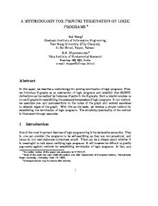
Parameter Estimation We partition the frames in the video sequence into two categories, “learning frames” and “general frames”. “Learning frames” are a set of initial frames for the model to learn the background. The “learning frames” help to initialise and form a Gaussian Mixture model. The parameters of the model formed using these frames are used to initialise the EM algorithm for the “general frames” (explained later). We have verified experimentally that 30-40 initial “learning frames” are sufficient for the background to be learnt. Frames following the “learning frames” are classified as “general frames”. Based on the type of frame, the parameter estimation technique differs (Fig. 1). For a “learning frame” (first 30-40 frames), the parameter updation technique is as follows: To begin the process, for each pixel position, each of the K Gaussians is intialised with a high standard deviation σi and a low prior weight ωi (i = 1, 2, ..., K). Subsequently, when any pixel from a “learning frame” comes in, it is checked against the existing K gaussians for a “match”. A match is found when the pixel value lies within 2.5 times the standard deviation of a particular distribution [7]. This threshold can be changed with little effect on performance. A variable threshold for each distribution is extremely effective in dealing with objects under different lighting conditions, as objects in low lighting exhibit lesser noise and therefore have a lower standard deviation as compared to objects in brightly lit regions. Having a threshold varying with the standard deviation therefore reduces the chance of erroneous detection. When a match is found then the parameters of gaussian mixture are updated using K-means approximation [7] as follows:

ωlnew = µnew l

N 1 X p(l|xi , Θg ) N i=1

PN

= Pi=1 N

xi p(l|xi , Θg )

i=1

(σl2 )new

PN =

i=1

p(l|xi , Θg )

p(l|xi , Θg )(xi − µnew )2 l PN g i=1 p(l|xi , Θ )

K

where l ∈ {yi }i=1 . yi identifies the Gaussian which generates the ith sample value, xi . That is, yi = r if xi belongs to the rth Gaussian in the mixture. The function p is defined using Bayes’ rule as: p(l|xi , Θg ) =

ωlg f (xi |θlg ) ωlg f (xi |θlg ) = PK g g p(xi |Θg ) r=1 ωr f (xi |θr )

where f is the Gaussian probability function, given by (2). It can be seen that at every iteration, the EM algorithm requires the complete history of the pixel process. This means that for the processing of the tth frame, all the frames from 1 to t − 1 need to be revisited. This is not practical for applications involving video segmentation. To avoid this, we use an approximation which only considers a window of a fixed number of frames as the history for the current frame. This ensures a consistent processing speed throughout the processing of the video. The EM algorithm is highly sensitive to initial parameters. A wrongly initialised EM algorithm may take longer, or may not even converge to the correct parameters. In our method, however, this problem is avoided as the EM algorithm is initialised using the parameters obtained by the online Kmeans approximation technique (after all the learning frames have been processed), which is a fairly suitable approximation.

ωt = (1 − α)ω(t−1) + α(Mt ) where Mt is 1 for the gaussian which matched and 0 for the remaining gaussians. 1/α defines the time constant which determines the speed at which the distribution’s parameters change. µ and Σ for the unmatched distributions remain the same. For the matched distribution, they as updated as: µt = (1 − ρ)µ(t−1) + ρXt 2 σt2 = (1 − ρ)σ(t−1) + ρ(Xt − µt )0 (Xt − µt )

where the second learning rate, ρ, is, ρ = αf (Xt |µ, σ)

Classification of pixels into background and foreground

If no match is found, then the least probable distribution to account for the new observation is replaced with a new distribution with mean as the value of the new observation, a high variance and low prior weight (ω). When the “learning” frames have been processed, the subsequent “general frames” update the gaussian mixture using

During the processing of a pixel, when the necessary parameters have been updated, the next step is to determine whether that pixel (in the current frame) is a part of the background or the foreground. We have adopted a classification technique similar to stauffer et al [7]. To understand the basis behind 3

Fig. 1: Summary of Steps involved in parameter estimation

the classification, let us first consider a pixel position, that has been part of the background process. The samples drawn from this process would be represented by one (or more) existing gaussian. Being a relatively static backgound, the samples would more or less be identical. Hence, the gaussians corresponding to them will have a low variance and high consistent evidence, ω supporting it. On the other hand, a foreground process may or may not even be represented by an existing distribution, and hence a new gaussian might have to be added to the existing mixture. In either case, the gaussian will definitely have low evidence supporting it and perhaps a high variance. Background distributions will therefore have high ω/σ values, whereas foreground pixels will have comparatively lower ω/σ values. ωi /σi (i = 1, 2, ..., K) values of the gaussians in the distribution can therefore be used to distinguish between background and foreground gaussians. To classify a pixel value into background or foreground, we use the following procedure. Firstly, based on the pixel value and the updated parameter values of the mixture model representing that pixel process, the probabilities of the pixel belonging to each of the gaussians in the mixture are calculated using:

(c)

(d)

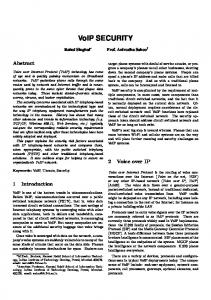
Fig. 2: (a) An original frame having high object-background contrast. (b) Its ground truth image. (c) Segmented image using k-means approximation on GMM [7]. (d) Segmented image using our approach. (e) Graphs showing Sensitivity and False Alarm Rate

IV. E XPERIMENTAL R ESULTS

In order to test the effectiveness of our algorithm for low contrast detection, several benchmark videos (provided by Advanced Computer Vision GmbH - ACV [8]) were used. The video sequences have the same background, but different shades of moving objects (hence different foregroundbackground contrast). The image size was fixed at 128x96 pixels and frame rate was fixed at 14fps. (Note: For clarity of display in print, the screenshots shown are negatives of the original images.)

where f represents the Gaussian probability density function. Let the gaussian having the highest probability (as obtained above) be called “P”. This means that the the current pixel value under consideration belongs to the gaussian “P”. Following this step, the all the distributions are theoretically organized based on their ω/σ values. Then the first B distributions are chosen as the background model, where B = argminb

(b)

(e)

pi (X) = f (X|µi , σi ), i = 1, 2, ..., K

b X

(a)

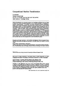
One of the most widely accepted techniques of object detection and tracking using background subtraction, proposed by Stauffer et al. [7], failed to segment objects under low contrast conditions (Fig. 3(c) and 4(c)). Only objects having high contrast with the background are detected effectively (Fig. 2(c)).

! ωk > T h

k=1

where T h is a measure of the minimum portion of the data that should be accounted for by the background. Let the remaining distributions which are not classified as background be denoted as “F”. If the distribution “P” is part of the distribution set “F” then clearly, the new pixel is part of the foreground. Else the pixel is classified as background.

However it can be seen that our approach effectively segments moving objects when the background-foreground contrast is low. (Fig. 3(d) and 4(d) ) 4

(a)

(b)

(a)

(b)

(c)

(d)

(c)

(d)

(e)

(e)

Fig. 3: (a) An original frame having a slightly lower objectbackground contrast. (b) Its ground truth image. (c) Segmented image using k-means approximation on GMM [7]. (d) Segmented image using our approach. (e) Graphs showing Sensitivity and False Alarm Rate

Fig. 4: (a) An original frame having a very low objectbackground contrast. (b) Its ground truth image. (c) Segmented image using k-means approximation on GMM [7] (no segmentation can be seen). (d) Segmented image using our approach. (e) Graphs showing Sensitivity and False Alarm Rate

Quantitative Analysis To better understand and analyse the results, we use quantitative measures of Sensitivity and False Alarm Rate. For the same, we first divide the pixels of any frame into 4 categories: True Positive (TP): Number of pixels which are actually foreground and are detected as foreground in the final segmented image. False Positive (FP): Number of pixels which are actually background but are detected as foreground in the final segmented image. True Negative (TN): Number of pixels which are actually background and are detected as background in the final segmented image. False Negative (FN): Number of pixels which are actually foreground but are detected as background in the final segmented image. We define, Sensitivity =

F alseAlarmRate =

FP FP + TN

A plot of Sensitivity gives a measure of the fraction of the actual background detected. We tested and compared our proposed method viz a viz the method proposed by Stauffer et al. [7] on three benchmark video sequences. We observe that in Fig. 2, where there is considerable contrast between the object and background, both the methods give appreciable results. In Fig. 3, the contrast is slighly lowered. We can see that very few regions are being segmented using k-means approximation on GMM [7]. Our method, however, yeilds far more superior results. In Fig. 4, there is extremely low contrast between the moving body and its background. None of the pixels got segmented using k-means approximation on GMM [7]. Our method still provides very appreciable results even in this case. This clearly demonstrates the robustness of our system in such conditions.

TP TP + FN

and 5

V. C ONCLUSION AND F UTURE W ORK

R EFERENCES

In this paper, we have successfully addressed the problem of detection and tracking of objects under low contrast conditions. We have successfully tested our system on a variety of videos involving different environmental conditions and having extremely low object-background contrast. We have also compared our algorithm with the more popular method of updating the mixture model via k-means approximation [7], and have obtained superior results. Due to the inherent advantage of using a Gaussian Mixture Model, our system has the ability to deal with multimodal distributions and adapt to lighting changes. The system has a very high potential to be used in applications involving military camouflage, detection and tracking of balls etc in sport events, tracking of hazed out objects at a large distance, among others. To further improve the performance of the tracker, we are focusing on two areas - speed and accuracy. We are using an approximation of the EM algorithm to save on processing time at the loss of some accuracy. Optimization of the algorithm used can lead to a further increase in the speed of convergence of the algorithm. To improve the accuracy of the detected object we are in the process of implementing a ’split and merge’ algorithm to reorganize the Gaussians in the mixture more optimally, which may yeild better results. Also, a self learning algorithm to dynamically determine the optimum number of Gaussians would make the system more adaptive.

[1] J Bilmes. A gentle tutorial of the em algorithm and its application to parametric estimation for gaussian mixture and hidden markov models. Technical report, Univ. Calif. Berkely, 1997. [2] D Davies, P.L Palmer, and M Mirmehdi. Detection and tracking of very small low-contrast objects. In Proceedings of the 9th British Machine Vision Conference, pages 599–608, September 1998. [3] A.P Dempster, N.M Laird, and D.B Rubin. Maximum likelihood from incomplete data via the em algorithm. Journal of the Royal Statistical Society, 39(1):1–38, 1977. [4] Y Raja, S McKenna, and S Gong. Segmentation and tracking using colour mixture models. In Asian Conference on Computer Vision, Hong Kong, pages 607–614, January 1998. [5] C Ridder, O Munkelt, and H Kirchner. Adaptive background estimation and foreground detection using kalman-filtering. In International Conference on Recent Advances in Mechatronics (ICRAM), UNESCO Chair on Mechatronics, pages 193–199, 1995. [6] N Saunier and T Sayed. A feature-based tracking algorithm for vehicles in intersections. In The 3rd Canadian Conference on Computer and Robot Vision, page 59, July 2006. [7] C Stauffer and W.E.L Grimson. Adaptive background mixture models for real-time tracking. In IEEE Conference on Computer Vision and Pattern Recognition, Colorado, USA, pages 599–608, June 1999. [8] Advanced Computer Vision GmbH. Motion detection video sequences. http://muscle.prip.tuwien.ac.at/data here.php. [9] C.R Wren, A Azarbayejani, T Darrell, and A Pentland. Pfinder: Real-time tracking of the human body. IEEE Transactions on Pattern Analysis and Machine Intelligence, 19(7):780–785, July 1997.

6