racy in arrow recognition [5, 3]. We already suggested [4] that it is better to detect arrows after the other symbols are detected. We proposed an algorithm, which ...
Detection of Arrows in On-line Sketched Diagrams using Relative Stroke Positioning Martin Bresler, Daniel Pr˚usˇa, V´aclav Hlav´acˇ Czech Technical University in Prague, Faculty of Electrical Engineering, Department of Cybernetics, 166 27, Praha 6, Technick´a 2, Czech Republic {breslmar, prusapa1, hlavac}@cmp.felk.cvut.cz
Abstract This paper deals with recognition of arrows in online sketched diagrams. Arrows have varying appearance and thus it is a difficult task to recognize them directly. It is beneficial to detect arrows after other symbols (easier to detect) are already found. We proposed [4] an arrow detector which searches for arrows as arbitrarily shaped connectors between already found symbols. The detection is done two steps: a) a search for a shaft of the arrow, b) a search for its head. The first step is relatively easy. However, it might be quite difficult to find the head reliably. This paper brings two contributions. The first contribution is a design of an arrow recognizer where the head is detected using relative strokes positioning. We embedded this recognizer into the diagram recognition pipeline proposed earlier [4] and increased the overall accuracy. The second contribution is an introduction of a new approach to evaluate the relative position of two given strokes with neural networks (LSTM). This approach is an alternative to the fuzzy relative positioning proposed by Bouteruche et al. [2]. We made a comparison between the two methods through experiments performed on two datasets for two different tasks. First, we used a benchmark database of hand-drawn finite automata to evaluate detection of arrows. Second, we used a database presented in the paper by Bouteruche et al. containing pairs of reference and argument strokes, where argument strokes are classified into 18 classes. Our method gave significantly better results for the first task and comparable results for the second task.
1. Introduction This paper deals with on-line handwriting recognition, where the input consists of a sequence of strokes. A stroke is a sequence of points captured by an ink-input device (the most commonly a tablet or a tablet PC) as the user was writing with a stylus or his finger. In handwriting recognition,
the research has already moved from recognition of plain text to recognition of a more structured input as diagrams. This work is focused on recognition of arrows in on-line sketched diagrams. Arrows are the most important symbols in diagrams, since they bear the most valuable information about the diagram structure – what symbols are connected together. However, it is a difficult task to recognize them because of their varying appearance. We consider two diagram domains – finite automata (FA) and flowcharts (FC). There is a freely available benchmark database available for each of the domains: the FA database [4] and the FC database [1]. Figure 1 shows examples of diagrams from these two domains. It is obvious that arrows can be arbitrarily directed and their shafts might be straight lines, curved lines, or polylines. Moreover, their heads have a different shape. There exists an approach, where arrows are detected first and the knowledge of arrows helps to naturally segment the rest of the symbols [14]. The problem is that authors of this approach put very strict requirements on the way the arrow is drawn. It must consist of one or two strokes and the arrow’s head must have only one predefined shape. Another approach is to detect arrows the same way as other symbols – using a classifier based on the symbol appearance. Since the arrows might be arbitrarily rotated and the heads might have different shapes, it is necessary to create several arrow sub-classes. This approach is more general, but the achieved accuracy is limited. The state-of-the-art methods in flowchart recognition achieve always very small accuracy in arrow recognition [5, 3]. We already suggested [4] that it is better to detect arrows after the other symbols are detected. We proposed an algorithm, which searches for arrows as arbitrarily shaped connectors between already found non-arrow symbols. It works in two stages: a) arrow shaft detection, b) arrow head detection. The detection of arrow head is based on heuristics and does not achieve satisfactory precision. In this paper, we employ machine learning to improve the proposed arrow detector with arrow head classifier based on relative strokes positioning.
(a)
(b)
Figure 1. Examples of hand-drawn diagrams containing arrows connecting symbols with rigid bodies: (a) finite automata, (b) flowchart.
In many cases, appearance does not give us enough information to classify single strokes and we need some contextual information. Relative position of a stroke with respect to a reference stroke is the most intuitive. Bouteruche et al. [2] addressed this problem directly and proposed a fuzzy relative positioning method. The authors introduced a method evaluating the relative position of strokes based on the fact how pairs of strokes fulfil a set of relations such as ”the second stroke is on the right of the first stroke” through defined fuzzy landscapes. They used this method to solve a prepared task, where pairs of reference and argument strokes are given and the argument strokes have to be classified into 18 classes corresponding to several types of accentuation or punctuation. The information about the appearance and the relative position of the argument stroke with respect to the reference stroke must be combined together to achieve a good recognition rate. This task adequately demonstrates the need for relative positioning system. They used Radial Basis Function Networks (RBFN) as a classifier. The method was further improved by a better definition of fuzzy landscapes and using SVM by Delaye et al. [7]. Although the fuzzy relative positioning is a powerful method useful for more complex tasks as recognition of structured handwritten symbols (Chinese characters) [6], it gives poor results when applied on arrow head detection. Our work brings two contributions. First, we define arrow head detection as a classification of possible arrow head strokes based on relative positioning. We used this arrow head classifier to significantly improve proposed arrow detector. Second, we propose a new method for evaluation of the relative position of strokes, which exploits simple low-level features and uses Bidirectional Long Short Term Memory (BLSTM) Recurrent Neural Network (RNN) as a classifier. The BLSTM RNN proved to be a good tool for classification of individual strokes [13]. The rest of the paper is organized as follows. Section 2 describes the proposed arrow detector and the way the relative positioning is exploited to determine which strokes
represent the head of the arrow. Section 3 introduces our method for evaluation of the relative position. Experiments and their results are described in Section 4. Finally, we make a conclusion in Section 5.
2. Arrow detector Arrows are symbols with a non-rigid body. They consist of two parts: shaft and head. The head defines the orientation of the arrow. However, arrow’s appearance can be changing arbitrarily according to the given domain. They can have various shapes, lengths, heads, and directions. Therefore, it is a difficult task to detect arrows with ordinary classifiers based on symbol appearance. However, each arrow connects two other symbols with a rigid body (see Figure 1). It is beneficial to detect these symbols first and leave the arrow detection to another classifier detecting arrows between pairs of these symbols. This new classifier must perform the following two steps: 1. Find a shaft of the arrow connecting the given two symbols. This shaft is just a sequence of strokes leading from a vicinity of the first symbol to a vicinity of the second symbol and it is undirected. 2. Find a head of the arrow, which is located around one of the end-points of the shaft. The head defines orientation of the arrow (if it is heading from the first symbol to the second symbol or vice versa). The detection of an arrow’s shaft can be done iteratively by simply adding strokes to a sequence such that the first stroke starts in a vicinity of the first symbol and the last stroke ends in a vicinity of the second symbol. A new stroke is added to the sequence only if the distance between the end-point of the last stroke and the end-point of the new stroke is smaller than a threshold. The algorithm must consider all possible combinations of strokes creating a valid connection between the given two symbols. The search
Ref.pointmA Pairsmofmsymbols
Detectionmofmarrowm shaft
Shaft
Querymstrokesm searchmandm classification
HeadmA
Extractionmofm referencemstrokesm andmpoints
Selectionmofmthembestm arrowmhead
Ref.mpointmB
Querymstrokesm searchmandm classification
Arrow
HeadmB
Figure 2. Arrow recognition pipeline. The recognition process is illustrated on a simple example of two symbols from FC domain.
space can be reasonably reduced by setting a maximal number of strokes in the sequence. This number depends on the domain and the fact, how many strokes users use to draw arrow’s shafts. Typically, it is four and two for flowcharts and finite automata, respectively. We can immediately remove some shafts, which are in a conflict with another shafts, and keep those with the smallest sum of the following distances: a) distance between the first symbol and the first stroke of the shaft, b) distance between the second symbol and the last stroke of the shaft, c) distances between individual strokes of the shaft. Since we do not know the orientation of the arrow yet and the shaft is undirected, we have to consider both endpoints of the shaft and try to find two heads (one in the vicinity of each end-point). Ideally we will be able to find just one head. In practice, it can happen that we find two heads and we have to decide which one is better. The detection of an arrow’s head is not a trivial task, because there might be a lot of interfering strokes around the end-points of the shaft: heads of another arrows or text. The decision which strokes represent the true arrow’s head we are looking for and which are not, is a task, where the stroke positioning might be beneficially used. First, we define a reference stroke (a sub-stroke of the shaft) and a reference point (end-point of the shaft), which are used to express a relative position of query strokes (details follow in Section 2.1). Second, this information about relative position is given to a classifier making the decision. The query strokes are all strokes in a vicinity of a given end-point of the shaft, which are not a part of the shaft itself nor the two given symbols. We make a classification into two classes: head and not-head. Explanation for the evaluation of the relative position of strokes and classification is given in Section 3. Let us just note that the classifier returns a class into which the query stroke is classified along with a potential. We use this potential to decide which head is of better quality in the case we find two. We just compute a sum of potentials of all strokes in each head and decide for the head with the bigger value. This slightly favours heads consisting of higher number of strokes, which is desirable in the most cases. A pseudocode for the algorithm that we just described is divided into two procedures and presented in the supplementary material as Algorithm 1 and Algorithm 2. The arrow recognition pipeline is depicted in Figure 2.
It happens quite often that the user draws a shaft and a head of an arrow by one stroke. Our algorithm would fail in that case. Therefore, we make one important step before we try to find the arrow’s head – we segment the last stroke of the shaft into smaller sub-strokes in such a way that the head is split from the shaft. Created sub-strokes are divided into two groups. One group is used to finish the shaft again such that it reaches the symbol again. Sub-strokes of the second group are put into the set of query strokes possibly forming the head. Our splitting algorithm is described in Section 2.2. If the shaft and the head are not drawn by one stroke, the algorithm will ideally perform no segmentation and this step can be skipped.
2.1. Reference stroke and reference point It is necessary to define a reference stroke. Position of all query strokes will be evaluated relatively with respect to it. Naturally, it seems that the arrow’s shaft should be the reference stroke. However, it is better to use just a sub-stroke of the shaft for this purpose. The reason is that the shaft might be arbitrarily curved or refracted, the whole arrow might be arbitrarily rotated, and we want to normalize the input in such a way that the reference stroke has always more or less the same appearance and the query strokes have always more or less the same relative position. Therefore, we create a sub-stroke beginning at the end-point of the shaft with a shape of a line segment. It is done iteratively by adding points to the newly created stroke until the value of a criterion, expressing how similar is the stroke to a line, is bigger than a threshold. The criterion is a ratio of the distance between the end-points of the stroke and the path length of the stroke (sum of distances between neighbouring points). We set the threshold empirically to 0.95. Another condition is that the distance between end-points of the stroke must be bigger then a threshold empirically derived from the average length of strokes, because the possible presence of so called hooks at ends of strokes would cause small value of the criterion for short strokes. Figure 3 illustrates how the reference stroke is determined as a sub-stroke of the shaft. Then we rotate the reference stroke and all query strokes by such an angle that the vector given by the end-points of the reference stroke will be pointing in the direction of the x-axis. In another words, it will cause that the true arrow heads should point from the left to the right. For purposes
of our method for evaluation of relative position of strokes (described in Section 3), we have to define a reference point. Obviously, it is the end-point of the shaft.
(a)
(b)
(d)
(c)
(e)
Figure 3. Example showing a diagram and the way of choosing the reference point, the reference stroke, and the rotation. Individual pictures illustrates the following: (a) whole diagram with a highlighted (red) arrow to be detected, (b) detected arrow’s shaft is blue and right end-point is considered to be the reference point, second point is green, the angle α used to rotate query strokes is marked, (c) rotation is done, the reference point is red as well as strokes of the real arrow’s head, (d) analogously to (b) with the other end-point considered, (e) analogously to (c) with exception that there is no real head, because the arrow’s orientation is wrong.
Because we still do not know the orientation of the arrow, we have to consider both options: the arrow is heading to the first symbol or the second symbol. Therefore, we define two reference points, end-points of the shaft. A reference (sub)stroke is associated to each of these two points then. Figure 3 shows the whole process of the reference stroke extraction and rotation.
2.2. Stroke segmentation Stroke segmentation is very important field of research, because it is frequently used preprocessing step. Therefore, there exist various papers dealing with this problem. The segmentation is done by defining a set of splitting points. The substantial information is curvature and speed defined at each point and geometric properties of stroke segments.
The common approach is to find tentative splitting points with high curvature and low speed. The best subset of these points is selected according to the error function fitting points of each segment into selected primitives. The most common primitives are line segments and arcs [8, 15]. It is also possible to use machine learning to train a classifier detecting the splitting points [9, 11]. The presented algorithms are sophisticated and allow to find segments fitting predefined primitives. However, using any of these methods seems to be an overkill for our task. We do not require to split a stroke at any precisely defined point nor to create segments with particular geometrical properties (line segments or arcs). All we need is to split the arrow’s head from its body and it is not important if both the body and the head will be further split into several segments. Therefore, we suggest to use much simpler algorithm for stroke segmentation. Its description follows. We compute a value AA, which we call “accumulated angle”, associated to each point of the stroke S = {p1 , p2 , . . . , pn } according to the following equation: AAi = mean(Rank3{A(i, 1), . . . , A(i, min(i−1, n−i, R))}), (1) where i is the index of the point in the sequence, Rank3 is an operator choosing up to the three smallest values of a given set, R is the maximal radius, and A is a function computing an angle between two vectors defined by the index of the given reference point and its two neighbouring points chosen by the size of the radius. The function A is defined as follows: A(i, r) = arccos
− −−→ −−−−→ p− i pi−r · pi pi+r . kpi pi−r k · kpi pi+r k
(2)
Let us note that AAi is computed according to Equation (1) only for i ∈ {2, . . . , n − 1} and AA1 = AAn = 0. We define the initial set of splitting points by taking points where the AA reached a local minima and the value is smaller than mCoeff · mean{AA1 , . . . , AAn }. In the case that there are two splitting points too close to each other (dist(pi , pj ) < distThresh), we remove one with smaller AA value. We set mCoeff = 0.5 and distThresh = 200 empirically. After this removal, the segmentation is done. We tested the described algorithm on arrows from the FA database (see Section 4.1) which were drawn by one stroke and it turned out that the algorithm split the head from the body in 100% of cases. Let us emphasize that parameters mCoeff and distThresh are tunable. It makes it easy to adjust for demands of a given task.
3. Evaluation of relative position of strokes Unlike the method by Bouteruche et. al, where a query stroke is evaluated with respect to the whole reference
p1
p1
p2 d1
d1
d2 α1 R αn
α2
x
dn
α1 R
dn
αn
pn
x
pn
(a) Arrow domain.
(b) Accent domain.
Figure 4. Example showing pairs of reference and query strokes and extracted sequences of features (angles and distances) for both domains. Reference point R is marked red. In the case of arrow domain, both, the reference and the query, strokes are already rotated. The query stroke is a sequence of points {p1 , p2 , . . . , pn }.
stroke by evaluating its fuzzy structuring element, we propose to evaluate the relative position of a query stroke with respect just to a single point of the reference stroke. In the case of arrows, it is the end-point of the arrow’s shaft. In the case of the task defined by Bouteruche et al., it can be an arbitrary fix point. We propose to choose a center of the reference stroke’s bounding box. We are given a reference stroke, which is represented by its reference point R and a query stroke S defined by a sequence of its points: S = {p1 , p2 , . . . , pn }. To describe the relative position of S with respect to R, we express relative position of each point pi using polar coordinates. Position −−→ − of each point is defined by the angle αi = Rpi ∠→ x and the distance di = kRpi k. We create a sample for each pair of a reference and query strokes consisting of a sequence of the described features {[α1 , d1 ], [α2 , d2 ], . . . , [αn , dn ]} and a label indicating the class of the query stroke. For illustration, see Figure 4. We propose to use (B)LSTM RNN as a classifier, because it reaches the best results in many applications. However, it is possible to use different tools for classifying sequences (e.g. Hidden Markov Models). When dealing with neural networks, it make sense to normalize inputs: vk − mk , (3) vˆk = σk where vk is an input value, vˆk is the normalized value, mk and σk are the mean and the standard deviation of all values of the same feature from the training database, respectively. We use this normalization to normalize the distance only. The advantage of proposed features is the fact that they are simple and easy to extract (low time complexity). Moreover, they express relative position of the query stroke with respect to the reference point as well as the shape of the query stroke. It is possible to reconstruct the trajectory of the query stroke from the sequence of features. It leads to simple implementation and fast evaluation.
4. Experiments We made experiments on two tasks. The first one is the task defined in this paper – classification of strokes into two classes head, not-head when the reference stroke is a part of the arrow’s shaft. The second task is to classify argument strokes representing accentuation or punctuation of its reference strokes into 18 classes. The task as well as the database called ACCENT was proposed by Bouteruche et al. In the case of arrows we additionally evaluated the whole process of arrows detection, where the stroke classification is a subtask. We used both positioning methods to solve both tasks and we made a comparison. All experiments were done on a standard tablet PC Lenovo X230 (Intel Core i5 2.6 GHz, 8GB RAM) with 64-bit Windows 7 operating system.
4.1. Arrows We used the FA database for this experiment. The version 1.1 contains the annotation of heads and shafts of arrows. We extracted a reference point and stroke for each arrow as described in Section 2.1. The only difference is that the shaft is known from the annotation. We created a set of query strokes and rotated these strokes according to the reference stroke. We extracted features with respect to the reference point or the reference stroke depending on the used method for each query stroke and assigned a label based on the annotation from the database. We refer to the samples with the label head as positive and those with the label not-head as negative samples. The FA database consists of 12 diagram patterns drawn by several users and it is split into training and test dataset. The training dataset contains diagrams from 11 users (132 diagrams) and the test dataset diagrams from 7 users (84 diagrams). Each diagram is formed of 54 strokes and contains 5 symbols and 10 arrows in average. We extracted 1480/834 positive and 1263/1019 negative samples from the training/test dataset. Arrows drawn by one stroke are manually segmented in the
For the method of Bouteruche et al., we used a RBFN implemented within the library Encog [10]. We set the number of the nodes in the hidden layer to be a power of the number of features, which leads to equally spaced RBF centers. It is the setting qiving the best performance. We tried two sets of features proposed by Bouteruche et al. referred in their paper by numbers 4 and 5 and we achieved the accuracy of 95.4 % and 88.2 %, respectively. It is not surprising that the feature set number 5 reached much worse results. It contains features expressing how much a query stroke fits into structuring elements of all classes. However, in this case, we have just two classes and the class of negative samples contains arbitrarily shaped strokes and thus the structuring elements are too wide. We also implemented the method by Delaye et al. [7]. Their filtered fuzzy landscape is an improvement of the Bouteruche’s feature set 5 and thus it gives rather low precision for the very same reason. The feature set number 4 gives much better results. However, it was still inferior in comparison with our method – the best overall precision of 95.36 %. For more detailed results see again Table 1. Since we use RNN in our method, the classification has higher time complexity (especially with increasing complexity of the net). The classification made by a RBFN is indeed very fast. On the other hand, it is much faster to extract the low level features we use: 0.016 ms per sample. Feature extraction is slower in the case of fuzzy positioning: 2.89 ms per sample for the feature set number 4 and 0.99 ms per sample for the feature set number 5.
99.5 99
precisionc[L]
For our method, we used LSTM and BLSTM RNNs implemented within the library JANNLab [12]. We tried different numbers of nodes in the hidden layer to get the best performance. We always trained the network in 200 epochs with the following parameters: learning rate 0.001, momentum 0.9. We achieved the best overall precision of 99.9 % with the BLSTM RNN with 32 nodes in the hidden layer. However, it might be important to find a trade-off between precision and time complexity and thus it might be better to use the LSTM RNN with only 8 nodes in the hidden layer, because it is significantly faster. It gives the precision of 99.6 % and the average time needed for classification is 0.79 ms. For details, refer to Figure 5. The best achieved precision for individual classes are given in Table 1. The achieved precision on the test2 with the best trained neural network was not decreased and reached 99.9 %.
PrecisioncofcRNNs 100
98.5 98 97.5 97 96.5 96 c 2
LSTM BLSTM 4 8 16 numbercofcnodescincthechiddenclayerc[−]
32
TimeLneededLtoLclassifyLoneLsample 7
6
5
timeL[ms]
database. However, to demonstrate our segmentation algorithm from Section 2.2, we created a second test dataset (ref. as test2), where we further segmented query strokes. Obtained sub-strokes created new samples with the same label as the original ones. We used this dataset to show that possible oversegmentation will not lower the final precision. We created 1252 positive and 1876 negative examples this way.
4
3
2
1
0L 2
LSTM BLSTM 4 8 16 numberLofLnodesLinLtheLhiddenLlayerL[−]
32
Figure 5. Dependency of precision and time complexity on the number of nodes in the hidden layer of RNNs for the FA database. Method Ours Bouteruche et al. (4) Bouteruche et al. (5) Delaye et al.
positive 99.91 % 98.56 % 94.24 % 95.17 %
negative 99.85 % 92.75 % 83.32 % 86.07 %
overall 99.88 % 95.36 % 88.24 % 90.17 %
Table 1. Comparison of precisions for arrow heads detection.
4.1.1
Arrow detector test
We took all annotated symbols with rigid bodies and tried to find arrows with the arrow detector we proposed (query strokes for arrow heads were classified with our best BLSTM RNN). We compared the detected arrows with annotated arrows. Let us remind that all pairs of symbols were considered. Conflicting arrow shafts were removed immediately. However, adding arrow heads may cause another conflicts. The result of the arrow detector is a list of arrow candidates and a structural analysis should be done to solve the conflicts. However, we tried to remove conflicts by simply keeping arrows with higher confidence to see how it affects recall and precision. The test dataset of the FA
database contains 796 arrows. We achieved the recall of 95.4 % / 94.2 % and the precision of 41.5 %/95.4 % for unperformed / performed conflict removal. Our arrow detector performs 106.5 stroke classifications in average per diagram while searching for arrow heads while there are 10 arrows in average per diagram. 4.1.2
to use spatial context – their relative position. The examples of the benchmark have been written on a PDA by 14 writers. The training database contains 4243 examples of 8 writers and the test database contains 2393 examples of 6 writers. None of the writers is common to both data sets.
Diagram recognition pipeline test
We embedded our arrow detector into the diagram recognition pipeline proposed earlier [4] and made experiments on the FA and FC databases. The FC database does not contain annotation of arrow heads and shafts. Therefore, we used the arrow head classifier trained on the FA database in both cases. The results are shown in Tables 2, 3. Although there is an improvement in both domains, it is more significant in the FA domain. The recognition accuracy increased in all symbol classes, which shows that misrecognized arrows can cause further errors in classification of other symbols. Class Arrow Arrow in Final state State Label Total
Correct stroke labeling [%] Previous Proposed 89.3 94.9 78.5 85.0 96.1 99.2 95.2 96.9 99.1 99.8 94.5 97.4
Correct symbol segmentation and recognition [%] Previous Proposed 84.4 92.8 80.0 84.0 93.8 98.4 94.5 97.2 96.0 99.1 91.5 96.4
Table 2. Diagram recognition results for the FA domain.
Class Arrow Connection Data Decision Process Terminator Text Total
Correct stroke labeling [%] Previous Proposed 85.3 88.7 93.3 94.1 95.6 96.4 90.8 90.9 93.7 95.2 89.7 90.2 99.0 99.3 95.2 96.5
Correct symbol segmentation and recognition [%] Previous Proposed 74.4 78.1 93.6 95.1 88.8 90.6 74.1 75.3 87.2 88.1 88.1 88.9 87.9 89.7 82.8 84.43
Table 3. Diagram recognition results for the FC domain.
4.2. Accent The Accent database consists of pairs of reference and argument strokes. The task is to classify the argument strokes into 18 graphic gestures. Two of them correspond to the addition of a stroke to a character. The 16 others (see Figure 6) correspond to an accentuation of their reference character (acute, grave, cedilla, etc.), to a punctuation symbol (coma, dot, apostrophe, etc.) or to an editing gesture (space, caret return, etc.). As several subsets of gestures have the same shape, the only way to discriminate them is
Figure 6. Classes of the argument strokes in ACCENT database.
To apply our method, we set a center of each reference stroke’s bounding box as a reference point and extracted features. We tried LSTM and BLSTM RNNs the same way as in the case of the Arrow database. However, we achieved the precision of 91.9 % only. It turned out that our features have a problem to distinguish very small argument strokes like acute, apostrophe, or dieresis. These strokes often consist just of one single point. Therefore, we decided to enrich the set of features and add local features describing the appearance of strokes. We used four features introduced by Otte et al. [13]: an index of the point to distinguish long and short strokes, sine and cosine of the angle between the current and the last line segment (zero for extreme points), and sum of lengths of the current and the previous line segments. Let us note that the point indices and distances are normalized (3). We refer to the two sets of features and associated experiments as basic and extended. We achieved the best precision with the extended features and the BLSTM RNN with 32 nodes in the hidden layer, which was 93.6 %. The training was done again with the learning rate of 0.001 and the momentum of 0.9. The ROC curves and time complexities are shown in Figure 7. In the case of the method of Bouteruche et al., we used our reimplementation and made the experiments. We confirm the results they stated – the precision of 95.75 %.
5. Conclusions We have shown how important and difficult task is the arrow recognition for the whole process of diagram recognition. We designed an arrow recognizer, which detects arrows in two steps: a) detection of an arrow’s shaft, b) detection of an arrow’s head. First step is easy, because the search for a shaft is guided by detected symbols connected by the arrow. For the second step, we proposed a novel arrow head
Acknowledgment
Precision%of%RNNs 100 90 80
Basic%LSTM Basic%BLSTM Extended%LSTM Extended%BLSTM
The first author was supported by the Grant Agency of the CTU under the project SGS13/205/OHK3/3T/13. The second and the third authors were supported by the Grant Agency of the Czech Republic under Project P103/10/0783 and the Technology Agency of the Czech Republic under Project TE01020197 Center Applied Cybernetics, respectively.
precision%[L]
70 60 50 40
References
30 20 10 % 2
4
8 16 32 number%of%nodes%in%the%hidden%layer%[−]
64
TimeBneededBtoBclassifyBoneBsample 3.5
3
BasicBLSTM BasicBBLSTM ExtendedBLSTM ExtendedBBLSTM
timeB[ms]
2.5
2
1.5
1
0.5
0B 2
4
8 16 32 numberBofBnodesBinBtheBhiddenBlayerB[−]
64
Figure 7. Dependency of precision and running time on the number of nodes in the hidden layer of RNNs for ACCENT database.
classifier based on relative stroke positioning. We presented a classification method based on low-level features using (B)LSTM RNNs. We embedded the proposed arrow detector into diagram recognition pipeline and we increased the accuracy of the state-of-the-art diagram recognizer on the benchmark databases of finite automata and flowcharts. We have also made the comparison with the state-of-theart method for relative positioning method. This method is unable to solve the proposed task adequately and reaches the inferior precision. However, we have made the comparison on the task for which this method was developed and it shows that our method gives slightly worse results in that case. It implies that the fuzzy positioning might be a good solution for some sort of tasks (data), but it is not a general tool. On the other hand, our method seems to be more general since it gave relatively good results in both cases. Even in the case it gives slightly worse results it might be a good alternative thanks to its simplicity and fast feature extraction.
[1] A.-M. Awal, G. Feng, H. Mouchere, and C. Viard-Gaudin. First experiments on a new online handwritten flowchart database. In DRR 2011, pages 1–10, 2011. [2] F. Bouteruche, S. Mac´e, and E. Anquetil. Fuzzy relative positioning for on-line handwritten stroke analysis. In Proceedings of IWFHR 2006, pages 391–396, 2006. [3] M. Bresler, D. Pr˚usˇa, and V. Hlav´acˇ . Modeling flowchart structure recognition as a max-sum problem. In Proceedings of ICDAR 2013, pages 1247–1251, August 2013. [4] M. Bresler, T. V. Phan, D. Pr˚usˇa, M. Nakagawa, and V. Hlav´acˇ . Recognition system for on-line sketched diagrams. In Proceedings of ICFHR 2014, pages 563–568, September 2014. [5] C. Carton, A. Lemaitre, and B. Couasnon. Fusion of statistical and structural information for flowchart recognition. In Proceedings of ICDAR 2013, pages 1210–1214, 2013. [6] A. Delaye and E. Anquetil. Fuzzy relative positioning templates for symbol recognition. In Proceedings of ICDAR 2011, pages 1220–1224, September 2011. [7] A. Delaye, S. Mac´e, and E. Anquetil. Modeling Relative Positioning of Handwritten Patterns. In Proceedings of IGS 2009, pages 122–127, 2009. [8] M. El Meseery, M. El Din, S. Mashali, M. Fayek, and N. Darwish. Sketch recognition using particle swarm algorithms. In Proceedings of ICIP 2009, pages 2017 – 2020, 2009. [9] G. Feng and C. Viard-Gaudin. Stroke fragmentation based on geometry features and HMM. CoRR, 2008. [10] Heaton Research, Inc. Encog Machine Learning Framework, 2013. http://www.heatonresearch.com/encog. [11] J. Herold and T. F. Stahovich. Classyseg: A machine learning approach to automatic stroke segmentation. In Proceedings of SBIM 2011, pages 109–116, 2011. [12] S. Otte, D. Krechel, and M. Liwicki. JANNLab Neural Network Framework for Java. In Proceedings of MLDM 2013, pages 39–46, 2013. [13] S. Otte, D. Krechel, M. Liwicki, and A. Dengel. Local feature based online mode detection with recurrent neural networks. In Proceedings of ICFHR 2012, pages 531–535, 2012. [14] A. Stoffel, E. Tapia, and R. Rojas. Recognition of on-line handwritten commutative diagrams. In Proceedings of ICDAR 2009, pages 1211–1215, 2009. [15] A. Wolin, B. Paulson, and T. Hammond. Sort, merge, repeat: An algorithm for effectively finding corners in handsketched strokes. In Proceedings of SBIM 2009, pages 93– 99, 2009.