Detection of Denial-of-Message Attacks on Sensor ... - Elaine Shi

Detection of Denial-of-Message Attacks on Sensor Network Broadcasts ∗ Jonathan M. McCune

Elaine Shi Adrian Perrig Michael K. Reiter Carnegie Mellon University {jonmccune, rshi, perrig, reiter}@cmu.edu

Abstract So far, sensor network broadcast protocols assume a trustworthy environment. However, in safety and missioncritical sensor networks this assumption may not be valid and some sensor nodes might be adversarial. In these environments, malicious sensor nodes can deprive other nodes from receiving a broadcast message. We call this attack a Denial-of-Message Attack (DoM). In this paper, we model and analyze this attack, and present countermeasures. We present SIS, a Secure Implicit Sampling scheme that permits a broadcasting base station to probabilistically detect the failure of nodes to receive its broadcast, even if these failures result from an attacker motivated to induce these failures undetectably. SIS works by eliciting authenticated acknowledgments from a subset of nodes per broadcast, where the subset is unpredictable to the attacker and tunable so as to mitigate acknowledgment implosion on the base station. We use a game-theoretic approach to evaluate this scheme in the face of an optimal attacker that attempts to maximize the number of nodes it denies the broadcast while remaining undetected by the base station, and show that SIS significantly constrains such an attacker even in sensor networks exhibiting high intrinsic loss rates. We also discuss extensions that permit more targeted detection capabilities.

1. Introduction Message broadcast is a fundamental communication primitive in most sensor networks. Researchers propose a variety of broadcast protocols [4, 17, 20, 22, 25, 28, 31]; however, all these protocols assume a trusted environment and fail in adversarial environments. Sensor networks de∗ This research was supported in part by CyLab at Carnegie Mellon under grant DAAD19-02-1-0389 from the Army Research Office, and grant CAREER CNS-0347807 from NSF, and by a gift from Bosch. The views and conclusions contained here are those of the authors and should not be interpreted as necessarily representing the official policies or endorsements, either express or implied, of ARO, Bosch, Carnegie Mellon University, NSF, or the U.S. Government or any of its agencies.

ployed in mission-critical environments require a secure broadcast protocol that is robust against attackers. In this paper, we study the Denial-of-Message Attack (DoM), where sensor nodes are deprived of broadcast messages. While nodes can fail to receive broadcasts due to benign network failures, here we consider the possibility that these failures are maliciously induced by an attacker. A simple approach is for every broadcast recipient to send an authenticated acknowledgment for each broadcast message. However, this approach results in a substantial load on the network to carry acknowledgments and on the base station to process them. This problem is well known as the ACK implosion problem in the reliable broadcast community [3, 15]. Thus, in the design of our algorithm, we place a premium on message savings, particularly on reducing the number of acknowledgments per broadcast. We propose Secure Implicit Sampling (SIS), an algorithm by which a broadcasting base station detects the failure of nodes to receive its broadcasts. We presume the attacker’s goal is to deny the broadcast to as many nodes as possible while remaining undetected by the base station. Our goal, then, is to limit the attacker’s capacity to achieve this, so that the attacker’s increased disruption of broadcasts results in an increased probability that he is detected, irrespective of the strategy he pursues. SIS allows us to detect a disruptive adversary and in the meantime, reduce the number of acknowledgments sent to the base station, by having a subset of recipients acknowledge each broadcast, where this subset is computed deterministically but in a way that is hidden from the attacker. If the cryptographic mechanisms we employ cannot be broken by the attacker, then the attacker can ascertain whether an uncompromised node should acknowledge a broadcast only by observing the node produce the acknowledgment. This, of course, is too late for the attacker to disrupt the node from receiving this broadcast. Moreover, if the attacker disrupts the acknowledgment, then this provides evidence of his presence to the base station. A focus of our analysis of SIS is evaluating the extent to which it constrains an attacker in realistic settings, where packet loss may be significant. Packet loss can confound the base station’s efforts to detect an attacker, because the

cause for an absent acknowledgment could be the network itself: either the broadcast could have failed to reach the recipient, or the recipient’s acknowledgment could have been lost in transit to the base station. Using detailed simulations of sensor networks to determine what we believe to be realistic loss behavior, we evaluate our acknowledgment protocol and show that it nevertheless significantly constrains an attacker. Related Work Several researchers have considered the problem of efficient broadcast or efficient flooding in wireless networks [4, 17, 20, 22, 25, 28, 31]. To increase robustness for point-to-point message delivery in sensor networks, researchers considered using multi-path routing, e.g., Deb et al. [8] and Ganesan et al. [12]. Deb et al. also consider the approach of measuring the reliability and dynamically adapting message routing based on the desired delivery probability [7]. However, all of these works assume a trusted environment and are not designed to resist attacks. Probabilistic solutions for counting receivers of messages have been proposed in the context of multicast group size estimation [11, 24]. Despite the sophistication of these techniques, they assume a trusted environment. Malicious nodes can easily deviate from these protocols, crippling their operation. Wood and Stankovic [30] study denial-of-service (DoS) attacks in sensor networks. They present numerous DoS attack opportunities. Deng et al. [9, 10], and Karlof and Wagner [16] have considered the problem of secure pointto-point routing in sensor networks. These works do not consider secure message broadcasts. Staddon et al. discuss the efficient tracing of failed nodes in sensor networks [27]. They assume all nodes have powerful and adjustable radios that can transmit at extended distances; in particular, the base station is able to broadcast a message to all nodes. They present algorithms to trace failed nodes in a trusted environment. Castellucci et al. and Nicolosi et al. propose schemes to enable the aggregation of acknowledgements in a multicast environment [5, 23]. Both schemes are based on public key cryptography, therefore they are not suitable for some severely resource-constrained sensor networks. Contributions This paper makes the following contributions:

station can specify which nodes should produce an acknowledgment (Section 6).

2. Attack Taxonomy In this section we describe the shortcomings of existing broadcasting protocols in adversarial environments. The purpose is to study potential techniques that may be valuable to a DoM attacker, whose intent is to prevent broadcast messages from reaching one or more nodes in the network.

2.1. Attacks Against Flooding

• We use a game-theoretic model and simulation to evaluate SIS, and show that it significantly constrains a DoM adversary even if he behaves optimally (Sections 4 and 5).

In an idealized no-loss network, blind flooding (every node always retransmits exactly once every unique message it receives) is wasteful, since individual nodes are likely to receive the same broadcast multiple times. In practice, however, blind flooding is a commonly used technique, since its inherent redundancy provides some protection from unreliable wireless networks. Still, blind flooding is vulnerable to attacks. Blocking Attack An attacker may seek to compromise a vertex cut set of nodes, thereby partitioning the network into two halves, with complete control over communications between the partitions. The attacker can then choose to block communications between the partitions. A partition can contain any nonzero number of nodes, so a single isolated node whose only link to the rest of the network is through an attacker who blocks messages, constitutes a vertex cut set. An attacker may find it difficult to compromise a sufficient number of nodes to obtain a vertex cut set, but he may be able to succeed with fewer compromised nodes, if he could leverage other attacks to prevent a broadcast from reaching one or more nodes. Attacks which can be used to achieve this goal are: Denial of Service (DoS) A malicious node may be able to induce its neighboring nodes to perform excessive computations through an algorithmic attack, preventing the nodes from retransmitting a broadcast in a timely fashion; or consume excessive battery power, dramatically weakening or eliminating the node’s ability to transmit messages. Jamming A malicious node may be able to set its radio to transmit continuously, or very frequently, such that it jams the radio receivers on its neighboring nodes. Since the neighboring nodes cannot receive intelligible messages, they will be unable to receive broadcasts. Framing Protocols to detect malicious nodes have been proposed where nodes cast votes to incriminate suspect nodes [21]. A malicious node successfully performs a framing attack 1 if it is able to get the network or base station to flag a legitimate node as malicious. Malicious nodes have incentives to vote against well-behaved nodes, so that the

• We devise extensions to our basic protocol, including a technique based on Bloom filters by which a base

1 In this context framing refers to the act of maligning another party without provocation or just cause.

• We introduce the Denial-of-Message Attack (DoM) to sensor networks and show how current broadcast protocols are vulnerable to it (Section 2). • We present Secure Implicit Sampling (SIS), which is to the best of our knowledge the first protocol to detect DoM attacks in sensor network broadcasts (Section 3).

votes of the well-behaved nodes are discredited at the base station. In essence, the malicious nodes frame the wellbehaved nodes. Rushing In blind flooding, nodes perform duplicate suppression by tracking the content of recent of broadcasts so that they do not retransmit the same message more than once. This is imperative since nodes are likely to receive the same message multiple times. An attacker can defeat an insecure (i.e., a simple unique identifier for each broadcast consisting of a sequence number) duplicate-suppression technique by performing the rushing attack [14]. In this attack, two or more malicious nodes are assumed to have a means of communicating which is faster than ordinary broadcast propagation. Alternatively, the malicious nodes can use a denial-of-service attack to slow down other nodes’ message propagation. The malicious node nearest the broadcast source rushes the broadcast to the far-away node, which alters the message’s content without altering the fields used for duplicate suppression and then retransmits the message in the far-away part of the network. This malicious message propagates to one or more nodes, which will then reject the legitimate message when it finally arrives due to duplicate suppression. Unfortunately, current rushing prevention mechanisms have a high communication and computation overhead [14]. Since the payloads of broadcast messages do not change as the message propagates, hash-based duplicatesuppression can be used to nullify such rushing attacks. That is, if each node uses the hash of the message payload to perform duplicate suppression, an altered and rushed message does not cause rejection of the legitimate message.

2.2. Weaknesses in Efficient Broadcast More efficient broadcast protocols other than blind flooding have been proposed. While most of the attacks on flooding which we review in the previous section also apply to these efficient broadcast mechanisms, we now study attacks specific to these efficient broadcast mechanisms. Cluster-based Flooding Cluster-based flooding protocols, e.g., [18, 20, 28], use various heuristics to identify a subset of nodes—the cluster-heads—to retransmit broadcasts in an attempt to reduce or eliminate redundant transmissions. The frequency with which clusters are reestablished influences a particular protocol’s susceptibility to the attacks we discuss. In blind flooding, it is necessary for a malicious node to somehow compromise a vertex cut set of nodes to perform a blocking attack against a partition of the network. In a clustering scheme, it is only necessary to prevent cluster-heads from forwarding messages, since ordinary nodes do not retransmit broadcasts. Thus, attackers that can DoS, jam, frame, or otherwise disable cluster-heads can be successful with far fewer compromised nodes. This also gives malicious nodes incentive to become cluster heads. To further exacerbate this weakness, many clustering protocols allow nodes to nominate themselves for the position of cluster-

head. Malicious nodes can always volunteer. Another insecure cluster-head selection scheme is based on the clusterhead volunteer with the lowest node ID. The malicious node can easily spoof its node ID such that it is always selected. Tree-based Broadcast Tree-based broadcast protocols, e.g., [4], typically build a spanning tree over the network, where the broadcast source is the root of the tree. In treebased protocols, only non-leaf nodes retransmit the broadcast message. Tree-based protocols are similar to clusterbased protocols if we look at the non-leaf nodes as cluster heads. Therefore, many attacks that work for clustering protocols also work for tree-based protocols. For the blocking attack, it will suffice to block non-leaf nodes. Malicious nodes can also violate the clustering protocol to get elected as non-leaf nodes to get an advantage. Conclusions The trend we see is that, as a protocol for flooding becomes more efficient, it also becomes more fragile and vulnerable to attack, since ever-fewer nodes retransmit broadcasts. Since efficiency was the primary goal of these protocols, little was done to secure the cluster-head selection process. Thus, the attacker can effectively partition the network by lying about selection criteria such that it always becomes the cluster-head or intermediate node.

3. Secure Implicit Sampling In this section, we describe Secure Implicit Sampling (SIS), a protocol to detect the Denial-of-Message Attack in sensor network broadcast. SIS uses controlled probabilistic checking to request message acknowledgments from a subset of nodes. Using cryptographic techniques, SIS constrains an attacker such that he is unable to guess ahead of time which subset of nodes are sampled. We also discuss how to tune the parameter of the sampling process to enable a tradeoff between the false positive and false negative rates. It is challenging to accurately classify broadcast message loss in a sensor network as the result of an attack, as opposed to collision or contention in wireless networks.

3.1. Assumptions We assume the existence of a base station which is considerably more powerful than ordinary sensor nodes in terms of computational power, storage, etc., but not in terms of radio transmission power. Specifically, we assume that the base station is able to perform on the order of 10 6 pseudorandom function computations in the time it takes for a broadcast message to propagate through the network and acknowledgments to propagate back. We assume the base station is the source of all legitimate broadcast messages. We also assume that a secure key-management protocol is present, e.g., [26], to establish and manage secure pairwise keys between each node and the base station.

3.2. The Basic Protocol We perform random sampling of broadcast acknowledgments. We have identified several security requirements for our sampling protocol: 1. It is necessary to apply appropriate cryptographic functions to ensure data origin authentication, i.e., the base station has to be sure which node sent the ACK and that it is not forged by some malicious node. 2. An attacker must have no way of finding out a priori which set of nodes are selected to send acknowledgments, otherwise a sophisticated attacker may selectively forward the message to the selected nodes. We introduce the following notation: • Msgs: The set of possible broadcast messages. We assume that each broadcast message that the base station sends is unique. • F : A pseudorandom function family F : Keys(F ) → Msgs → Range(F ) parameterized by a secret value K ∈ Keys(F ). We write F (K, m) for F (K)(m). Informally, if K is randomly chosen from Keys(F ), then an attacker not knowing K cannot distinguish F (K) from a randomly chosen function from Msgs to Range(F ), even after seeing F (K, m) for many values m ∈ Msgs of its choosing. In practice, a pseudorandom function family is often implemented using a block cipher, e.g., AES [6]. F • Ksk : A key randomly chosen from Keys(F ) that is shared between the broadcast source and the node k.

• fp (x): A function f p : Range(F ) → {0, 1} such that |{x ∈ Range(F ) : fp (x) = 0}| ≈ p·|Range(F )|. That is, fp is a function for which the fraction of inputs that map to 0 is p, and 1 − p map to 1. • MAC: A function family MAC : Keys(MAC) → Msgs → Range(MAC) parameterized by a secret value K ∈ Keys(MAC). We write MAC(K, m) for MAC(K)(m). MAC is a message authentication code: Informally, if K is randomly chosen from Keys(MAC), then an attacker not knowing K cannot produce MAC(K, m) for any m ∈ Msgs, even after having seen MAC(K, m
) for many m
= m of its choosing. In practice, a common MAC implementation is the HMAC algorithm [1]. MAC • Ksk : A key randomly chosen from Keys(MAC) that is shared between the broadcast source and the node k.

Based on our security requirements, we propose the following protocol: Upon receiving a broadcast m from the F , m)) = 0. base station s, node k tests whether f p (F (Ksk MAC If so, it sends a = MAC(Ksk , m) to s. We assume node k authenticates each broadcast m as coming from the base station. Note that upon the reception of a message, it is implicit which set of nodes are selected to acknowledge. In fact, each node can be viewed as being selected independently with probability p. This method rules out the need to send explicit ACK requests to selected nodes, reducing the communication overhead. When the base station s receives an acknowledgment a purportedly from node k for broadcast m, it confirms that MAC MAC(Ksk , m) = a. For a particular round i, let S i be the number of ACKs expected, R i the number of ACKs received and confirmed. The base station can compute S i F by checking f p (F (Ksk , m)) = 0 for every node in the network. This is efficient based on our assumption that the base station can efficiently compute on the order of 10 6 pseudorandom functions. If R i /Si < h, where h is a threshold value, an alarm is raised. Note that h is not necessarily a constant, it may also be a function of S i . If we assume no packet loss or node failures, h = 1, i.e., an attack is signaled if R i < Si . In the real world where probabilistic packet loss comes into play, it is challenging to determine the right threshold value used to signal an attack; setting it too high will give rise to excessive false positives (signaling an attack when there is none), while setting it too low will result in a high false negative rate (attackers being able to escape detection). We propose to use a training phase, where the base station performs a test of the network when it is most likely to be functioning correctly, e.g., immediately after the sensor network is deployed. This normal lossy situation is used as a baseline for comparison in the detection phase. In this way, we tune our threshold to account for normal packet losses. Changes in the natural loss rate of the network following completion of the training phase will have a negative impact on the accuracy of our detection scheme. Malicious nodes performing a DoM attack are motivated to remain undetected for as long as possible, thus they never drop acknowledgments (the acknowledging node has already received the broadcast) and they always send back acknowledgments when sampled.

3.3. Analysis Our analysis is based on the assumption that missing acknowledgments are caused by network load or malicious activity; we assume there are no node failures. We first analyze the ideal world, where there is no packet loss (0-loss). In this world, there are no false positives; any lost acknowledgment implies an attack. Let x be the number of victim nodes and p the probability that a node gets sampled (selected to return an acknowledgment). Then the probability

of detection could be calculated as follows: Pr0 loss (detection) = 1 − (1 − p)x Though the 0-loss assumption does not hold in practice, the above calculation is useful in the sense that: 1) it is straight-forward and gives us intuition about the effectiveness of the scheme; 2) it is an upper-bound for the probability of detection in the lossy world; 3) it approximates the probability of detection well when packet loss rate is small. The false negative rate is one minus the probability of detection: Pr0 loss (false negative) = 1 − Pr0 loss (detection) = (1 − p)x We now consider the real world, lossy case. We introduce the basic model for our detection system, explain how to set the threshold value, and analyze the false positive and detection rate of our system. We use a training phase to obtain an estimate of the natural loss rate of the network. For this purpose we make the following assumptions. We assume that the network operates under a stable environment (i.e., network topology and radio properties are fixed and do not vary over time), and all other activities of the sensor network aside from the broadcast (e.g., routing updates) remain stable over time. Let pi be the probability that the base station receives an ACK from the i th node given that it is sampled. The failure to receive an expected acknowledgment may either arise from the probabilistic loss of an outbound message or the loss of an incoming acknowledgment. We do not explicitly distinguish between these two cases in our model. We assume that lost ACKs from different receivers are independent of each other. In reality, losses may be correlated due to local radio interference or other networking errors. We plan to consider correlated message losses in future work. pi will vary for each node i because each node is in a different position (i.e., number of hops away from the base station, number of neighbors, etc.) in the network. In reality, due to the additional radio resource contention the acknowledgments bring in, p i is dependent on the particular set of nodes sampled. However, when the sample size is relatively small as compared to the network size, the effect of the acknowledgments on the wireless medium is negligible. Therefore, we can assume that regardless of what subset of nodes are sampled, each p i will remain stable. The problem reduces to the following: we have n different coins, where coin i has probability p i of flipping heads. We randomly choose s out of n coins and flip them. Let R be the number of “heads” among the s coins. It is easy to show that as n → ∞, R → Binomial (s, pr0 ), where pr0

n 1
= · pi n i=1

. Therefore, under our model, the number of ACKs received approximates a binomial distribution over p r0 and Si , where Si is the number of expected ACKs in round i, and pr0 is defined by the expression above. Intuitively, p r0 is the probability an expected ACK is received. In addition, 1 − pr0 reflects the natural loss rate of the network under normal conditions. In Appendix A, we show how well this simplistic model approximates our simulation scenario. In reality, different networks may exhibit entirely different characteristics, so it is important to choose a model that reflects the actual network characteristics. In the training phase, the base station will obtain an estimate of pr0 . Assume the training phase consists of r rounds. The number of nodes sampled in each round is S 1 , . . . , Sr , and the number of ACKs received is R 1 , . . . , Rr . Thus r Ri pr0 ≈ i=1 (1) r i=1 Si In the detection phase, the base station first computes S i for each round by going through all nodes in the network. In the presence of an attack, the observed R i will deviate from the anticipated Binomial (Si , pr0 ) distribution. Therefore, to flag an attack, we could perform the following hypothesis test: H0 : pr ≥ pr0

vs. H1 : pr < pr0

where pr is the estimate of the probability that an expected ACK is lost from the observed R i . Let T = Pr( ≤ Ri ACKs received | Si sampled ) Ri  
Si = · (pr0 )j · (1 − pr0 )Si −j . j j=1 Reject H0 if T < α, where α represents the false positive rate of the detection scheme. The probability of detection grows with the impact of the attack. We quantify the attacker’s impact with x, the number of deprived nodes in one round of broadcast. Note that the packet delivery performance of a real sensor network is probabilistic, thus an attacker’s influence is also probabilistic. While x is the number of deprived nodes, we are unable to determine exactly which of them are the direct victims of the attack and which are caused by probabilistic loss. In spite of this, x is a straight-forward measure of the attacker’s impact. For any test we use, it is possible to rewrite the rejection rule as: R i < f (Si ), where f (Si ) is a function of S i . Particularly, for the aforementioned test using the binomial distribution: f (Si ) = max { t,t∈Z

t  
Si j=1

j

· (pr0 )j · (1 − pr0 )Si −j < α}

(1 − p1 , 1) =

Pr(detection) – n » X Pr(Ri < f (s)|Si = s) · Pr(Si = s)

(p1 , 0) 1

...

s=0

=

«– n » s „ X X Pr(Si = s) Pr(Ri < f (s)|Q = q) · Pr(Q = q)

s=0

≥

=

s X

–

Undetected

P r(Ri < f (s)|Q = q)P r(Q = q)

q=s−f (s)+1

n

`n−x´`x´ – »“ ” min(x,s) X n s s−q q n−s `n´ p (1 − p) s s s=0 q=max(s−n+x,s−f (s)+1) n X

min(x,s) n »“ ” X X n s p (1 − p)n−s s s=0 q=max(s−n+x,s−f (s)+1)

Figure 1. Derivation of the probability that an attacker is detected. Si is the number of sampled nodes in a particular round i; Ri is the number of received ACKs; Q is a random variable denoting the number of deprived nodes in the sampled subset; n is the network size; x the number of deprived nodes; p the probability each node is sampled. Note that when we use a reliable routing protocol to route back the ACKs, the "≥" sign in the third line is strictly "=".

Figure 1 derives the probability that an attack is detected. Note that in the 0-loss world, f (s) = s, and the expression in Figure 1 simply reduces to Pr(detection) = 1 − (1 − p)x . Also, when packet loss is negligible, i.e., pr0 ≈ 1, we can use Pr(detection) = 1 − (1 − p)x to approximate the probability of detection.

4. The Optimal Attacker We consider an attacker whose goal is to deprive nodes of broadcast messages. His success is defined in terms of the number of legitimate nodes deprived of a broadcast. Without a detection system, the payoff for such an attacker is proportional to the number of deprived nodes. Therefore, if the attacker is able to selectively compromise any node in the network, his best strategy is to compromise all neighbors of the base station. In this way, he can cut off all the rest of the network from the base station, and achieve maximum payoff conveniently. If SIS is present, a simplistic attacker as described above will no longer be successful. The attacker’s chances of being detected by SIS increase with the number of deprived nodes. Once the attacker is detected, his payoff goes to zero as the system will start attack countermeasures. Thus a clever attacker will try to remain undetected with high probability while still doing damage to the network. In reality, the attacker’s optimal strategy depends on the attack coun-

Detected

(1, 0)

(1 − pk , k) (pn , 0)

(1 − pn , n)

`n−x´`x´ – s−q q `n´ s

(pk , 0)

k

...

n » X P r(Si = s)

s=0

=

q=0

Figure 2. Markov Decision Process (MDP) for the attacker. In the undetected state, the attacker has 1 . . . n possible actions, i.e., depriving 1 . . . n nodes. Each arrow is labeled with the tuple (p, r), where p is the probability and r is the reward.

termeasure we perform upon detection of malicious behavior. In the analysis that follows, we assume a simple model where once detected, the malicious nodes’ payoff goes to zero. In this section, we analyze SIS from a game theoretic perspective. We model the attacker with a Markov Decision Process (MDP) as shown in Figure 2.

4.1. Attacker Reward Function In a particular round i, the attacker’s immediate reward ri is the number of victim nodes in round i, if he has escaped detection by the end of round i; and 0, if he was detected in or before round i. The attacker’s total reward is defined as: J = r0 + γr1 + γ 2 r2 + γ 3 r3 . . . ∞
= γ i ri i=0

where γ is the discount factor, γ < 1, meaning the attacker always attaches less importance to a future reward. The attacker’s action is indicated by x, the number of victim nodes per round. His total discounted reward J is a function of x: J(x)

= E[Total reward | x victim nodes per round] = Pr(false neg.|x victim nodes) · (x + γJ(x))

yielding J(x) =

x · Pr(false neg.|x victim nodes) 1 − γ · Pr(false neg.|x victim nodes)

(2)

80

60

maximum total discounted reward optimal number of victims per round

maximum total discounted reward optimal number of victims per round (discounted sum of) # nodes

(discounted sum of) # nodes

70 60 50 40 30 20

50

40

30

20

10

10 0 0

0.1

0.2

0.3

0.4

p: probability each node gets sampled

(a) γ = 0.95

0.5

0 0

0.1

0.2

0.3

0.4

0.5

p: probability each node gets sampled

(b) γ = 0.8

Figure 3. Attacker’s maximum expected discounted reward as a function of p in the 0-loss world.

Note that when γ = 0, the attacker is only concerned about maximizing his immediate reward, and his reward function reduces to: J(x) = x · Pr(false neg.|x victim nodes) When γ = 1, the attacker attaches equal importance to his immediate reward and future reward, and his reward function reduces to: J(x) =

x · Pr(false neg.|x victim nodes) Pr(detection|x victim nodes)

This is his expected immediate reward in a single round multiplied by the expected number of rounds before he is detected. We now study the optimal behavior of the attacker in the no-loss case. The attacker’s reward function reduces to: J(x) =

(1 − p)x · x 1 − γ(1 − p)x

p is the probability each node gets sampled. Let x ∗ be the point where J(x) reaches its maximum J ∗ . Figure 3 plots x∗ and J ∗ against p. The two plots correspond to γ = 0.95 and γ = 0.8 respectively. We can see that as γ becomes small, i.e., the attacker is more concerned about his shortterm reward, the optimal attacker tends to deprive more nodes in the current round, and he will remain in the network for a relatively short time (as indicated by the distance between the dashed curve and the solid curve).

sampled) grows. In other words, as p grows, we are paying the price of increased transmission overhead for higher security guarantees. This is not necessarily true, however, in the real world with natural packet loss. In the real world, we expect pr0 to eventually decrease as p increases, i.e., as we transmit more acknowledgments for each broadcast, the network will be operating at a higher load, and we expect a higher level of congestion and packet loss. Therefore the effect of acknowledgments is two-fold in a real sensor network: 1) it causes more network congestion and hence a higher “natural” loss rate of the broadcast message; 2) it gives us a probabilistic guarantee on the delivery of the message. Thus in the real world, the attacker’s gain will no longer be monotonically decreasing as a function of p, and paying the price of higher transmission overhead will not always yield additional security. We now use a game-theoretic perspective to analyze this tradeoff. Consider the attacker and our detection system as two players in a zero-sum game, i.e., the gain of the attacker is the loss of our system. The attacker is entitled to choose x,2 while our system chooses p. Let J(p, x) be the attacker’s payoff function. The equilibrium of the game, ω, is given by the following minimax construction: ω = min

max J(p, x)

0≤p≤1 1≤x≤n

4.2. Reward Analysis

The above analysis will enable us to tailor our p for different network settings. Once the network is deployed, i.e., the layout of nodes, radio and environmental factors are determined, the base station can test the network and obtain an estimate of pr0 under different choices of p. The test

For the no-loss case, the attacker’s maximum expected reward decreases as p (the probability that a given node is

2 In practice, the attacker may not be so powerful as to have full control over x. However, an intelligent attacker will try his best, with his available resources, to approximate x∗ , the analytical optimal strategy.

1

should be performed in the absence of an attacker. Then the base station can use the minimax construction to determine the optimal p value for this particular setting. We will use this game-theoretic analysis when we compare simulation results with the expected behavior based on the analysis.

We have developed extensions to GloMoSim [29] to simulate SIS with blind flooding. Our extensions also model attackers that drop broadcast messages.

0.99

ACK Ratio

5. Simulation Results

0.995

0.985 0.98 0.975 0.97 0.965

5.1. Motivation We want our simulations to resemble actual radio performance. In particular, modeling packet reception as a simple radius based on ideal radio-range will yield unrealistic results. The probability of reception at node B of a packet transmitted from node A to node B demonstrates a heavy tail, remaining above 0 well beyond the advertised range of a given radio. Still, the probability never reaches 1.0, even if the nodes are extremely close [13]. Constructing an analytical model of this kind of environment is an open research challenge, thus, we use simulation to confirm our analytical results.

5.2. Setup To achieve the desired realistic behavior, we have performed all of our simulations with radio noise accumulation enabled in GloMoSim [29]. We use the default GloMoSim values for the remaining network device parameters. We find that the reachability behavior of our simulated broadcasts is similar to the behavior observed in experiments conducted on actual sensor nodes [13]. For each data point, we use at least 20 simulation runs. We configured GloMoSim to use a Bellman-Ford routing protocol to route acknowledgements back to the base station. At the beginning of each simulation run, we allow sufficent time for the table exchanges necessary in this distance-vector protocol to stabilize. During each individual experiment, the topology remains constant, minimizing the need to send routing updates. For each experiment, we first randomly generate a network topology. Then, we ran simulations with no attackers to derive the parameter p r0 , as defined in Equation 1. Note that pr0 obtained in this way will account for the natural loss rate, including any message loss due to collision or contention from the acknowledgment routing protocol overhead. After obtaining p r0 , we ran many simulation rounds with varying percentages of randomly compromised nodes. Each compromised node sends back an acknowledgement if sampled, but compromised nodes do not forward any broadcast messages. The analysis of the optimal attacker in Section 4 demonstrates the tradeoffs an attacker makes when trying to

0.96 0

10% 20% 30% 20

40

Round

60

80

100

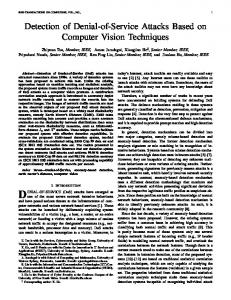
Figure 4. Smoothed ratio of received to expected acknowledgements computed at the base station for varying percentages of malicious nodes after the 49th broadcast. Parameters: 100 rounds of broadcast, n = 100 nodes, area = 2000m × 2000m, window size = 5, 20 different randomly generated topologies for each line.

achieve his goals. In particular, finding the optimal set of nodes the attacker should compromise is intimately tied to a particular network topology. Our analysis of SIS is based on the number of deprived nodes, rather than the number of attacking nodes. This serves to decouple our detection results from the attacker model and broadcast protocol we used. For our experiments, the network density was rather low—few nodes had more than five neighbors within radio communication range. This case benefits the attacker, since a commonly considered goal of the attacker is to create a vertex cut set of compromised nodes, partitioning the network.

5.3. Results In this section, we study the impact of the DoM attack on broadcast protocols. We are interested in the case where the attacker has compromised sufficiently many nodes to have a significant impact on how many legitimate nodes receive the broadcast message. Since flooding is the most general and widely used broadcast algorithm, we consider flooding in this section. As a sufficient number of nodes are compromised, their impact becomes evident. As the number of victim nodes in mid-sized networks (hundreds of nodes) increases, the attacker’s impact on the network becomes detectable by SIS. First, we present a naive example to convey the intuition behind detection. Figure 4 illustrates the ratio of received

0.15

1

0.125

False Positive Rate

Probability of detection

0.8

0.6

0.4

0.2 Simulation Theoretical

0 0

50

100

150

200

250

0.075

0.05

0.025

300

Number of deprived nodes

Figure 5. Probability of detection of the Denial-of-Message Attack based on the number of nodes deprived of the broadcast. Network size n = 600 nodes, area = 4898m × 4898m, p = 0.10, α = 0.05. After simulation, we calculated pr0 = 0.788327 to generate the theoretical curve.

to expected acknowledgments as computed at the base station. After the 49 th broadcast, some percentage of nodes are randomly chosen to be malicious. The impact on the ratio of received to expected acknowledgements is evident, as is the unique level of natural loss for each topology. Thus, an effective threshold that can be used to detect an attack is dependent on the natural loss characteristics of the particular topology, and configuring a scheme to detect attackers in sensor network broadcast is best done post-deployment. SIS-based Detection Figure 5 illustrates the detection capabilities of SIS in simulation, and compares those results with the theoretically expected performance, based on the p r0 (defined in Equation 1) observed in 0-attacker broadcast rounds. We performed the experiment on a simulated network containing 600 nodes. We used the same randomly generated topology for multiple simulation runs, while varying which nodes were malicious. We first ran hundreds of rounds of broadcast with no attackers to obtain p r0 , and then thousands of rounds with various percentages of attackers to generate a large set of victim nodes. We analyze the simulation output based on the number of deprived nodes in the network. For each number d of deprived nodes out of n total nodes, we collected the number of attack detections (true positives) and the number of non-detections (false negatives). Thus, for a given d: P r(detect ) =

0.1

detected attacks occurrences of d

In Figure 5, the probability p that each node gets selected to return an acknowledgment is 0.10. We set the parame-

0 0

0.025

0.05

0.075

α

0.1

0.125

0.15

Figure 6. Simulated false positive rate. 2000 rounds of simulations were run on a network with n = 600 nodes, area = 4898m × 4898m, p = 0.10. The first 200 rounds of broadcast were used for training, the rest were used for computing the false positive rate.

ter α = 0.05 for the hypothesis test (see Section 3.3) so that SIS-based detection yields a low rate of false positives. The simulations show that the actual probability of detection closely follows our analytical result. Figure 6 depicts the false positive rate we observed. The x-axis represents α, the theoretical false positive rate. α is used to pick the threshold of detection. The y-axis shows the simulated false positive rate (the number of false positives over 2000 rounds of broadcast to 599 nodes). During simulation, we observe behavior in approximately 0.2% of all rounds where almost none of the nodes receives a broadcast message. After some investigation, we conclude that this is due to the broadcast message being lost on the first hop, because the base station has a collision. Since we use a flooding algorithm for broadcast, as the message propagates beyond the first hop, more redundancy is introduced, and such dramatic message losses are less likely to happen. In our simulation, if such dramatic message losses happen in the training rounds (where we calculate the natural loss rate, p r0 , for the network), we eliminate them from the training data. We included the rounds with dramatic message loss in Figure 6, which plots the false positive rate. Optimal Attacker In Section 4, we introduced the idea that increasing p may not necessarily increase security. As the number of acknowledgments destined for the base station increases, the traffic load on the nodes nearest the base station also increases. Thus, we see a higher natural loss rate, and p r0 decreases. A decrease in p r0 indicates that the network is becoming more unreliable, hence unpredictable, which ben-

efits the attacker. In other words, the certainty with which the base station classifies missing acknowledgments as the result of natural loss, or the result of an attack, decreases. This suggests that there may be some values of p for which our random acknowledgment scheme will actually outperform a scheme where all nodes send acknowledgments for every broadcast (p = 1.0). Figure 7(a) shows the results of an experiment to test whether an increase in p results in a decrease in p r0 . Indeed, we see an increase in natural losses (p r0 decreasing) as more nodes are randomly selected to acknowledge (p increasing). It is the goal of SIS-based detection to minimize an attacker’s ability to increase his disruption of the network without increasing his probability of detection. In Section 4, we used a game theoretical analysis to show that there exists a min-max point where the attacker’s payoff can be minimized. Our result from the previous section suggests that the optimal point will not be at p = 1.0, which one might suspect from the analysis of the 0-loss network. Figure 7(b) compares the attacker’s optimal payoff in the 0-loss world with experimental results in the lossy world. The payoff function we use is the discounted reward function given in Equation 2, where the probability of detection is what we calculated in Figure 1. For the lossy world curve, we label the min-max point which shows the optimal p SIS-based detection should use for this particular topology. Thus, we have shown that the optimal p for SIS in a lossy, realistic network, is likely to be less than 1.0. The value was typically between 0.10 and 0.15 for the topologies we observed.

Each node’s acknowledgment takes the form of a message authentication code (MAC) computed with a secret key shared only between that node and the base station: MAC MAC , m), where Ksi denotes a shared key beMAC(Ksi tween the base station and node i. Naive schemes requesting explicit acknowledgments from all nodes will result in acknowledgment implosion as messages near the base station. However, if nodes can aggregate acknowledgments as they near the base-station, network overhead will be minimized. Consider a tree-based broadcast protocol, where acknowledgments traverse the reverse path that the broadcast traversed on its way through the network. Upon receiving acknowledgments from its children, each parent node can compute the XOR of its acknowledgment with those of all its children, and forward the resulting data up the tree towards the base station. For example, node i, with child nodes j and k, will compute the following: MAC ACKi = MAC(Ksi , m) ⊕ ACK j ⊕ ACK k

Node i will then forward ACK i up the tree towards the base station. Upon receiving acknowledgments from all of its neighbors, the base station can then compute the XOR of all received acknowledgments. If all nodes received the broadcast, and all aggregated acknowledgments arrived at the base station, then the base station can compute: ACK 1 ⊕ ACK 2 ⊕ . . . ⊕ ACK n

In this section, we examine possible extensions and alternative approaches to SIS.

where ACK i denotes the acknowledgment message from node i, in a network of n nodes (node 0 is the base station). The base station can locally calculate an expected value for the XOR of all acknowledgments by iterating through the keys it shares with each node for the purpose of computing acknowledgment MACs. If this locally computed aggregate acknowledgment matches the aggregate acknowledgment calculated from the acknowledgment messages received over the network, then the base station knows that all of the nodes in the network must have received the broadcast. This scheme is efficient if the expected performance of the network is such that all messages and acknowledgments can be expected to arrive. That is, it does not provide much useful information in the event that the locally computed aggregate acknowledgment does not match that computed from network data.

6.1. Exclusive-Or Aggregation

6.2. Acknowledgment Aggregation

The base station may sometimes require a high level of assurance that all nodes have received a broadcast. Consider, for example, a binary code update to nodes to correct a programming error discovered post-deployment. Without the update, nodes may become useless. We now present a scheme that leverages the exclusive-or (XOR) of MACs to efficiently receive acknowledgments from all nodes.

Each receiver has a buffer to store the latest t messages. Once a node is selected to return an ACK, it acknowledges all t messages in its buffer instead of only the most recent one. This allows the base station to collect more information in one acknowledgment. ACK aggregation enables delayed detection of an attack in a past round. Consider a node k, who is deprived of the

5.4. Limitations Although we used the number of deprived nodes (as opposed to the number of malicious nodes) as our metric for the severity of an attack, our simulation results may still be tied to the use of blind flooding for broadcast and the introduction of randomly selected malicious nodes. A sophisticated attacker may compromise nodes in such a way as to most readily achieve his goal.

6. Extensions and Discussion

1

80

Attacker’s Maximum Discounted Reward

simulated pr0 linear regression 0.99

pr0

0.98

0.97

0.96

0.95

0.94 0

0.1

0.2

0.3

0.4

0.5

p

(a) More acknowledgements cause a higher natural loss rate. Based on simulation data of 200 nodes randomly spread over an area of 2828m × 2828m. For each p we ran 600 rounds of broadcast.

Simulated Loss 0 Loss Fitted Curve

70 60 50

minmax point 40 30 20 10 0 0

0.1

0.2

0.3

p

0.4

0.5

(b) The game theoretical optimal strategy for the attacker and SIS under simulated packet loss rate. γ = 0.8, α = 0.05.

Figure 7. Impact of natural loss rate on the optimal attacker.

6.3. Reducing the Verifier’s Computational Overhead Basic SIS requires that the verifier run through all receivers in the network, computing F with every receiver, for each round of broadcast. Therefore, the computational overhead of the verifier is proportional to the number of receivers in the network. Thus far we have assumed that the base station is the broadcast source as well as verifier. Since a base station is usually a powerful node, we have not been concerned about the computational overhead. However, there might be scenarios where reducing the O(n) computational cost is useful, e.g., in ad-hoc or sensor networks without a central entity such as a base station, or where an ordinary node is required to perform the verification task.

1 0.9 0.8

Probability of detection

message in round i; and node k happens to be sampled in round i + δ, 0 < δ ≤ t. SIS-based detection may be able to discover the past attack δ rounds later, provided that k is not deprived again in round i + δ, in which case it will not be able to send back information about round i. This is acceptable, since the missing ACK in round i will be detected. To illustrate the benefit of using ACK aggregation, consider a simple binary attacker, operating in a 0-loss network. The attacker controls x downstream nodes; in each round of broadcast, he either drops packets so that all x downstream nodes are deprived of the message, or he relays the message such that all x downstream nodes receive it. Figure 8 evaluates the ACK aggregation scheme in terms of the probability of detection after some broadcast rounds. Refer to the Appendix B for the detailed derivation on which this figure is based.

0.7 0.6 0.5 0.4 0.3

buffer size = 1 buffer size = 2 buffer size = 3 buffer size = 4

0.2 0.1 0 0

5

10

15

20

# of rounds

Figure 8. ACK aggregation scheme: probability of detection after x rounds of broadcast. Each curve is for a different buffer size. When buffer size = 1, ACK aggregation reduces to the basic scheme.

We propose the following extensions to our basic scheme to alleviate the verifier’s computational overhead. Using a Unified Threshold While the basic scheme requires that the verifier go through all nodes in the network to determine the set of sampled nodes, it is possible to skip this step and still achieve a fair detection rate. In our detection system, each node gets sampled independently with probability p for each broadcast round. If we assume that in the

acknowledgment with probability (p ack · pcheck ), with respect to detection rate. Table 1 illustrates the tradeoff between transmission and computational overhead using random checking.

1 0.9

CDF of Ri without prior knowledge of Si posterior CDF of R knowing S = 33 i

i

0.8 0.7

6.4. Random Testing with Varying Probability

0.6 0.5 0.4 0.3 0.2 0.1 0 0

5

10

15

20

25

30

Figure 9. Cumulative Distribution Function of Ri with and without prior knowledge of S i . Network size n = 300, p = 0.1, pr0 = 0.95.

In our previous discussions, we have used a uniform sampling probability throughout the network. Sometimes, however, we may want to specifically check a network area. For instance, certain network regions may have stricter security requirements than others. In these scenarios, we want to associate different regions with a different sampling probabilities. One way to achieve this is through area-based keys [19]. By attaching to a message a MAC computed with an area-based key, the base station can broadcast to the corresponding region of nodes, effectively tuning their sampling probability.

6.5. Explicit Acknowledgment Requests 0-attacker world, an ACK will be received from any sampled node with probability p r0 , then we can obtain the prior distribution function for R i (the actual number of ACKs received in round i) without knowledge of S i (the number of sampled nodes). Based on the prior distribution of R i , we can obtain a unified threshold for R i , regardless of S i , to use as the rejection rule. Note that, in comparison, the threshold of rejection in the basic scheme is a function of S i . In the unified threshold scheme, for every incoming ACK, the verifier still needs to check whether the acknowledging node is actually sampled. However, as shown in Figure 9, the prior distribution of R i has larger variance than the posterior distribution when S i (number of nodes sampled in round i) is known. This weakens the precision of our detection system, i.e., if we fix the false positive rate, then using the unified threshold will yield a higher false negative rate. To reduce the false positive rate, we can relate the R i ’s in multiple recent rounds, and check whether they are a good fit of the hypothetical distribution. Note that here we assume that the attack is continual, i.e., if there is an attack in one particular round, it is likely that there is an attack in recent rounds as well. Random Acknowledgment + Random Checking One can apply the random testing idea twice:

The base station may need to explicitly request a set of nodes to acknowledge in each broadcast round. For instance, at some point, the base station might suspect that parts of the network are being attacked. Therefore, it may want to perform a more thorough survey of the suspicious region. Explicit acknowledgment requests instructing relevant nodes to return acknowledgments or reports in the next few rounds can be used to obtain this information. We must ensure that attackers eavesdropping on broadcast messages cannot ascertain which nodes are selected to send acknowledgments, or the attacker may selectively forward broadcast messages to only those nodes. Bloom filters [2] can be used to encode a set of nodes from which the base station explicitly wants acknowledgments. Let k1 , k2 , . . . , kt be the t nodes from which the base station wants an acknowledgment. Let H 1 , H2 , . . . , Hu be the u hash functions of the Bloom filter, each with range {1, . . . , v}. Let  = (b1 , b2 , . . . , bv ) be a bit vector of length v.  is the Bloom filter we attach to the message, and it is initially set to 0. Then the base station goes through the following construction:

1. Random Acknowledgment: the broadcaster randomly selects a subset of nodes to sample (return ACKs);

2. ∀i, 1 ≤ i ≤ t, ∀j, 1 ≤ j ≤ u, the base station computes Hij = Hj (MACi ), and sets bHij = 1.

2. Random Checking: the verifier randomly picks a subset of nodes to check whether they are sampled, and if so, whether they have indeed returned an ACK. Assume that the impact of the ACKs on the wireless communication medium is negligible. Then random acknowledgment with probability p ack in combination with random checking with probability p check equals random

1. ∀i, 1 ≤ i ≤ t, the base station computes MAC i = MAC MAC MAC(Ksi , m), where Ksi is another shared key between the base station and node k i .

For node k that receives the message, it performs a MAC membership test: it computes MAC(K sk , m), hence H1 (MAC), . . . , Hu (MAC); if all of these positions are 1 in the Bloom filter, then node k knows it is required to send back an acknowledgment in this round. Note that the Bloom filter may induce a small number of false positives, i.e., a few unsampled nodes may pass the

Scheme random ACK + random checking random ACK

Transmission Overhead n · p ack n · pequiv

Computational Overhead n · pcheck n

Table 1. Use of random checking to enable trade-off between computational and bandwidth resources. The two schemes in the table are equal in terms of detection rate (p equiv = pack · pcheck ), assuming acknowledgments have negligible impact on the wireless communication medium. p ack is the probability of selection of a given node to return a random acknowledgment; p check is the probability of selection of a given node by the verifier for checking; and n is the network size.

membership test and therefore believe that they are supposed to acknowledge. On the other hand, Bloom filters ensure that there are no false negatives, i.e., all sampled nodes are guaranteed to pass the membership test. In practice we can tune our u and v parameters to enable tradeoff between messaging overhead, computational overhead, and false positive rate. Given the Bloom filter, an adversary cannot figure out which set of nodes are selected, as long as the shared keys between the base station and each node are kept secret. This prevents him from selectively forwarding the message only to nodes that are sampled. We use a broadcast authentication protocol such as µTESLA [26] to authenticate the message and the Bloom filter. This prevents an attacker from arbitrarily altering the Bloom filter, e.g., setting every bit to 1 in order to perform a DoS attack.

6.6. Catching the Malicious Node After the verifier in a sensor network has detected the DoM attack, it may be desirable to identify the malicious node(s). We present a simple approach for identifying the malicious node. We start by using a fine-grained network diagnosis to identify the scope of damage. We observe that victim nodes in a DoM attack are usually geographically correlated, i.e., if one node is found to have missed the message, its neighbors are likely to be victims too. If the base station knows the topology of the network, it could do an expanding ring search to identify the region under attack. For example, if the base station detects that node A is deprived of a broadcast message, it explicitly queries all of A’s neighbors to determine whether they have received the message. In this way, the base station expands its search for every deprived node it finds, by querying all that node’s neighbors. The malicious node must be on the boundary of the affected region. We may now use a voting protocol to find the malicious node. The voting protocol requires that each node keep watch over its neighbors’ behavior in each broadcast, so that when a DoM attack is detected, the base station could poll the nodes near the boundary of the victim region. For instance, consider an attacker dropping packets in a blind flooding protocol. Since each node is supposed to re-

lay the message, if node A notices that its neighbor B is not relaying the message, it may vote that node B is malicious. In more complex protocols such as some cluster-based protocols [17, 20, 28], it is harder to define what constitutes malicious behavior. Additionally, a sophisticated attacker M may attempt to frame legitimate nodes, i.e., to make them look like attackers so that their votes against M will be discredited. In such cases, it is more difficult to distinguish a legitimate node from a malicious one.

7. Conclusion and Future Work Despite the importance of broadcast communication in sensor networks, so far no secure broadcast communication protocols have been proposed that can withstand attacks. In this paper, we introduce the Denial-of-Message Attack (DoM) in sensor networks and show how current broadcast protocols are vulnerable to it. In the presence of message loss, detecting a stealthy attacker is a challenge, as we show in this paper. We present Secure Implicit Sampling (SIS), which is to the best of our knowledge the first protocol to detect DoM attacks in sensor network broadcasts. We use a game theoretic model to evaluate SIS, and show that it significantly constrains a DoM adversary even if he behaves optimally. Our paper represents a first step in this important area. While SIS provides a general mechanism that allows us to sample a subset of network nodes for acknowledgments in a way hidden from the adversary, we do not stipulate what algorithm to use in practice for setting alarm thresholds and performing attack response, since thresholding and attack response algorithms should fit the needs of the specific application in concern. However, we do propose a basic model based on which we study the behavior of the optimal attacker. Though our model agrees well with the simulation scenario, it has several limitations. First, we assume that the network operates under stable conditions and nodes are immobile. We also assume that nodes do not fail over time. Second, we assume that lost acknowledgments are uncorrelated, which may not hold in some networks. We would like to address these limitations in future work and we anticipate that this paper will encourage other researchers to start working in this important area.

8. Acknowledgments We gratefully acknowledge support, feedback, and fruitful discussions with Lujo Bauer, Abtin Keshavarzian, Arati Manjeshwar, Bhaskar Srinivasan, Jimeng Sun, and Lakshmi Venkatraman. We also thank Charles Fry for his invaluable assistance in managing the simulator. We would also like to thank the anonymous reviewers for their helpful comments and suggestions.

References [1] M. Bellare, R. Canetti, and H. Krawczyk. Keying hash functions for message authentication. In Proceedings of Advances in Cryptology (Crypto), pages 1–15, 1996. [2] B. Bloom. Space/time trade-offs in hash coding with allowable errors. Communications of the ACM, 13(7):422–426, 1970. [3] J. Byers, M. Luby, M. Mitzenmacher, and A. Rege. A Digital Fountain approach to reliable distribution of bulk data. In Proceedings of the ACM SIGCOMM Conference on Applications, Technologies, Architectures, and Protocols for Computer Communication, pages 56–67, 1998. [4] M. Cagalj, J.-P. Hubaux, and C. Enz. Minimum-energy broadcast in all-wireless networks: NP-completeness and distribution issues. In Proceedings of the ACM Conference on Mobile Computing and Networking (MobiCom), Sept. 2002. [5] C.Castellucci, S.Jarecki, and G.Tsudik. Verifiable and secure acknowledgement aggregation. In Proceedings of Fourth Conference on Security in Communication Networks (SCN), Sept. 2004. [6] J. Daemen and V. Rijmen. The Design of Rijndael. SpringerVerlag, 2002. [7] B. Deb, S. Bhatnagar, and B. Nath. Information assurance in sensor networks. In Proceedings of the ACM Conference on Wireless Sensor Networks and Applications (WSNA), pages 160–168, Sept. 2003. [8] B. Deb, S. Bhatnagar, and B. Nath. ReInForM: Reliable information forwarding using multiple paths in sensor networks. In Proceedings of the IEEE Conference on Local Computer Networks (LCN), Oct. 2003. [9] J. Deng, R. Han, and S. Mishra. INSENS: INtrusion-tolerant routing in wireless SEnsor NetworkS. Technical Report CUCS-939-02, Department of Computer Science, University of Colorado, Nov. 2002. [10] J. Deng, R. Han, and S. Mishra. A performance evaluation of intrusion-tolerant routing in wireless sensor networks. In Proceedings of the IEEE Workshop on Information Processing in Sensor Networks (IPSN), pages 349–364, Apr. 2003. [11] T. Friedman and D. Towsley. Multicast session membership size estimation. In Proceedings of IEEE Infocom, Mar 1999. [12] D. Ganesan, R. Govindan, S. Shenker, and D. Estrin. Highly resilient, energy-efficient multipath routing in wireless sensor networks. Mobile Computing and Communication Review (MC2R), 5(4):10–24, 2002. [13] D. Ganesan, B. Krishnamachari, A. Woo, D. Culler, D. Estrin, and S. Wicker. Complex behavior at scale: an experimental study of low-power wireless sensor networks. Technical Report 02-0013, Computer Science Department, UCLA, July 2002.

[14] Y.-C. Hu, A. Perrig, and D. Johnson. Rushing attacks and defense in wireless ad hoc network routing protocols. In Proceedings of the ACM Workshop on Wireless Security (WiSe), Sept. 2003. [15] IETF RMT Working Group. Reliable multicast transport (RMT) charter. http://www.ietf.org/html. charters/rmt-charter.html. [16] C. Karlof and D. Wagner. Secure routing in wireless sensor networks: Attacks and countermeasures. In Proceedings of the IEEE Workshop on Sensor Network Protocols and Applications, May 2003. [17] H. Lim and C. Kim. Flooding in wireless ad hoc networks. Computer Communications, 24, Feb. 2001. [18] C. R. Lin and M. Gerla. Adaptive clustering for mobile wireless networks. IEEE Journal of Selected Areas in Communications, 15(7):1265–1275, 1997. [19] D. Liu and P. Ning. Location-based pairwise key establishments for relatively static sensor networks. In Proceedings of ACM Workshop on Security of Ad Hoc and Sensor Networks (SASN), Oct. 2003. [20] W. Lou and J. Wu. On reducing broadcast redundancy in ad hoc wireless networks. IEEE Transactions on Mobile Computing, 1(2):111–122, Apr. 2002. [21] S. Marti, T. Giuli, K. Lai, and M. Baker. Mitigating routing misbehaviour in mobile ad hoc networks. In Proceedings of the Conference on Mobile Computing and Networking, pages 255–265, Aug. 2000. [22] S.-Y. Ni, Y.-C. Tseng, Y.-S. Chen, and J.-P. Sheu. The broadcast storm problem in a mobile ad hoc network. In Proceedings of the ACM Conference on Mobile Computing and Networks (MobiCom), Aug. 1999. [23] A. Nicolosi and D. Mazires. Secure acknowledgment of multicast messages in open peer-to-peer networks. In Proceedings of International Workshop on Peer-to-Peer Systems (IPTPS), pages 233–248, Feb. 2004. [24] J. Nonnenmacher and E. W. Biersack. Scalable feedback for large groups. IEEE/ACM Transactions on Networking, 7(3):375–386, 1999. [25] E. Pagani and G. Rossi. Reliable broadcast in mobile multihop packet networks. In Proceedings of the ACM Conference on Mobile Computing and Networking (MobiCom), pages 34–42, 1997. [26] A. Perrig, R. Szewczyk, V. Wen, D. Culler, and J. Tygar. SPINS: Security protocols for sensor networks. In Proceedings of the ACM Conference on Mobile Computing and Networks (MobiCom), July 2001. [27] J. Staddon, D. Balfanz, and G. Durfee. Efficient tracing of failed nodes in sensor networks. In Proceedings of the ACM Workshop on Wireless Sensor Networks and Applications (WSNA), 2002. [28] I. Stojmenovic, M. Seddigh, and J. Zunic. Dominating sets and neighbor elimination-based broadcasting algorithms in wireless networks. IEEE Transactions on Parallel and Distributed Systems, 12(12):1– 12, Dec. 2001. Correction to pseudocode available at http://www.csi.uottawa.ca/ ivan/wireless.html. [29] M. Takai, L. Bajaj, R. Ahuja, R. Bagrodia, and M. Gerla. Glomosim: A scalable network simulation environment. Technical Report 990027, UCLA, Computer Science Department, 1999. [30] A. Wood and J. Stankovic. Denial of service in sensor networks. IEEE Computer, pages 54–62, Oct. 2002.

[31] Y. Yi, M. Gerla, and T. J. Kwon. Efficient flooding in ad hoc networks using on-demand (passive) cluster formation. In Proceedings of the ACM Symposium on Mobile Ad Hoc Networking and Computing (MobiHoc), 2002.

A The Binomial Distribution Assumption Figure 10 is a visual representation of how well the binomial model fits simulation result under three different sample sizes. As is conjectured, the figure demonstrates that the binomial model fits well when the sample size is small; however, as the sample size increases, the simulation curve tends to deviate from the binomial distribution. Also the simulation distribution tends to have larger variance than the fitted binomial distribution, which can be explained by the correlation between the sampled nodes that our model does not account for.

B

Derivation for ACK aggregation

In Section 6.2, we discussed using ACK aggregation to enable delayed detection of past attacks. We considered a simple binary attacker who has x downstream nodes in his charge; in each round of broadcast, he can choose to either relay or drop message to all x nodes. Let k be the buffer size in the ACK aggregation scheme. Define state as a bit vector of length k, (b 0 , b1 , . . . , bk−1 ). Let t denote the current round, then b i = 0 denotes that the attacker passes the message in round t − i; and conversely b i = 1 if he withholds the message in round t − i. Let p dr (1) denote the probability that the attacker drops the message in any round, and let pdr (0) = 1 − pdr (1) denote the probability that the attacker passes the message. Let pn (b0 , . . . , bk−1 ) denote the probability of no detection in a certain round, given that the state in this round is (b 0 , . . . , bk−1 ). Note that here detection includes detecting an attack in the past k rounds. Then  → − 1 if (b0 , . . . bk−1 ) = 0 pn (b0 , . . . , bk−1 ) = otherwise (1 − p)x where p is the probability each node gets sampled, and x is the number of victim nodes. Define p (i) (b0 , . . . , bk−1 ) as the probability that there is no detection until round i and that the state in round i is (b 0 , . . . , bk−1 ). For p(i) (b0 , . . . , bk−1 ), we have the following recursive formula. p(i) (b0 , . . . , bk−1 ) =

1


p(i−1) (b1 , . . . , bk−1 , b) · pdr (b0 ) · pn (b0 , . . . , bk−1 )

b=0

Initially, let  p(0) (b0 , . . . , bk−1 ) =

1 0

→ − if (b0 , . . . bk−1 ) = 0 otherwise

Then we can apply the above recurrence formula to compute the probability of detection after any number of rounds. The result is shown in Figure 8.

1

1

Fitted Binomial Simulation

0.9

Cumulative Distribution Function

Cumulative Distribution Function

0.9 0.8 0.7 0.6 0.5 0.4 0.3 0.2

0.8 0.7 0.6 0.5 0.4 0.3 0.2 0.1

0.1 0 0

Fitted Binomial Simulation

5

10

15

20

25

30

0 0

35

Number of ACKs Received

10

20

(a) Si = 31

50

60

70

1

Fitted Binomial Simulation

Cumulative Distribution Function

Cumulative Distribution Function

0.9

0.8 0.7 0.6 0.5 0.4 0.3 0.2

Fitted Binomial Simulation

0.8 0.7 0.6 0.5 0.4 0.3 0.2 0.1

0.1 0 0

40

(b) Si = 67

1 0.9

30

Number of ACKs Received

25

50

75

100

Number of ACKs Received

(c) Si = 150

125

150

0 0

50

100

150

200

Number of ACKs Received

(d) Si = 200

Figure 10. Cumulative distribution of number of received ACKs, where S i denotes the number of nodes sampled per round. The simulation involves 600 nodes spread over an area of 4898 × 4898m2.