The International Archives of the Photogrammetry, Remote Sensing and Spatial Information Sciences, Volume XLI-B3, 2016 XXIII ISPRS Congress, 12–19 July 2016, Prague, Czech Republic
DETECTION OF GEOMETRIC KEYPOINTS AND ITS APPLICATION TO POINT CLOUD COARSE REGISTRATION ∗
M. Buenoa, , J. Mart´ınez-S´ancheza†, H. Gonz´alez-Jorgea‡, H. Lorenzob§ a
School of Mining Engineering, University of Vigo, R´ua Maxwell s/n, Campus Lagoas-Marcosende, 36210 Vigo, Spain b School of Forestry Engineering, University of Vigo, Campus A Xunqueira s/n., 36005 Pontevedra, Spain Commission III, WG III/2
KEY WORDS: Point Cloud, Coarse Registration, 3D Keypoints Extraction, ICP, Geometry Description, LiDAR
ABSTRACT: Acquisition of large scale scenes, frequently, involves the storage of large amount of data, and also, the placement of several scan positions to obtain a complete object. This leads to a situation with a different coordinate system in each scan position. Thus, a preprocessing of it to obtain a common reference frame is usually needed before analysing it. Automatic point cloud registration without locating artificial markers is a challenging field of study. The registration of millions or billions of points is a demanding task. Subsampling the original data usually solves the situation, at the cost of reducing the precision of the final registration. In this work, a study of the subsampling via the detection of keypoints and its capability to apply in coarse alignment is performed. The keypoints obtained are based on geometric features of each individual point, and are extracted using the Difference of Gaussians approach over 3D data. The descriptors include features as eigenentropy, change of curvature and planarity. Experiments demonstrate that the coarse alignment, obtained through these keypoints outperforms the coarse registration root mean squared error of an operator by 3 - 5 cm. The applicability of these keypoints is tested and verified in five different case studies.
1.
INTRODUCTION
Data acquisition via static terrestrial laser scanners provides important advantages. State of the art devices are easy to manipulate and move from one position into another. The obtained LiDAR point clouds are, usually, ready to use, allowing regular users to work immediately with the devices and the data. The main drawback presented by this kind of technology is that the scanning device needs to be placed in different locations in order to obtain the complete scene. This fact is certain not only for outdoor scenes, but also for large and multiple rooms indoor buildings. Consequently, further preprocessing is needed to work over these scanned datasets. For example, the complete 3D reconstruction of the scene or the semantic classification and identification of objects in the point clouds, requires that all the scans are referred to a common reference frame. The automation of such task, usually, relies on the use of artificial targets placed along the scene (Franaszek et al., 2009, Akca, 2003). These markers are coded and easily identifiable inside the scanned data, allowing specific software to be able to register all the point clouds into the same coordinate frame. The last described procedure, even if it not necessary, requires that the operator possesses some expertise or trainee to be able to place the targets efficiently. Additionally, some situations present a difficulty to place the markers, like structures impossible to access by the operators. In these cases, manual alignment is the standard procedure. Another approach, that still requires work, is the use of natural targets that already are presented in the structures, like corners, signs, salient characteristics, etc. Some of these characteristics can lead to the generation of keypoints, which is one of the main aims of this manuscript. ∗ Corresponding
author:
[email protected]
†
[email protected] ‡
[email protected] §
[email protected]
This manuscript tries to demonstrate the use of a series of keypoints, which are obtained from point features information, in order to generate satisfactory results in coarse registration, and to outperform the results obtained by a human operator. The manuscript covers a brief review of the state of the art on point description and feature, and keypoint extraction of related techniques in Section 2, focused on the coarse registration application. Section 3 presents the proposed methodology to obtain those keypoints and perform the coarse registration. Subsequently, Section 4 provides the experimental procedure and results obtained using the proposed methodology. Finally, Section 5 shows the conclusions obtained from the performed work.
2.
STATE OF THE ART
One of the most extended strategies used for the coarse registration of point clouds without the use of any kind of artificial markers is defined in (Rusu, 2010, Theiler et al., 2014b, Gressin et al., 2013). First of all, the scanned point clouds are preprocessed to obtain salient features, compute point descriptors that are strongly related to these features, or even keep some points that are descriptive by themselves. Then, the point cloud is reduced to a sparse set of points representing the keypoints of the mentioned features. The last step of this particular procedure, relies on the matching of the keypoints in the overlapping area, mostly via their descriptors or their geometric properties, to obtain a rigid transformation matrix. This operation allows to align to one reference coordinate system that is roughly aligned for all the point clouds in the dataset. The results of this coarse registration, typically serves as the input to the standard fine registration algorithm which is represented by the Iterative Closest Point (ICP) algorithm (Besl and McKay, 1992). Although there exist others approaches proposed to solve this topic, like (Brenner et al., 2008, Von Hansen, 2006) where the use of planar surfaces is exploited to obtain the registration, this manuscript is focused
This contribution has been peer-reviewed. doi:10.5194/isprsarchives-XLI-B3-187-2016
187
The International Archives of the Photogrammetry, Remote Sensing and Spatial Information Sciences, Volume XLI-B3, 2016 XXIII ISPRS Congress, 12–19 July 2016, Prague, Czech Republic
on the keypoints and point features. This work covers the keypoints extraction and keypoint-based coarse registration from 3D geometries. Thus, the rest of this section reflects the different and most popular approaches to describe and detect the keypoints that represent the sparse subsample of the original point clouds.
be small enough for the larger radius, while for a point that belongs to a corner, the entropy should be high enough for a small radius. The point features can represent the linearity, planarity, scattering, omnivariance, anisotropy, eigenentropy, and change of curvature.
2.1
This work is focused on the application of these point features in order to obtain a subsampled point cloud that can be used to perform coarse point cloud registration. Among the previous mentioned characteristic, these point features are easy to implement, and do not require a huge amount of time to compute. Also, the storage capacity is relatively small. In Section 3. a description of the used point features is given in more detail. For the rest of the point features, authors would like to refer to the original works.
Point Features
The ability of a system to obtain certain characteristics of the points that belong to a point cloud is an important field of study. Nowadays, there exist several systems that try to understand and give an interpretation of the scene and the surroundings where it is being used. The majority of the points in a point cloud represent an object, a part of the room or the environment. Most of the relevant used techniques work computing the information from a neighbourhood around each point obtaining a value which represents the geometric type where it belongs. There are several point descriptors and features that help to give an interpretation of the scanned data. Rusu et al. (Rusu et al., 2008) developed a point descriptor that helps to identify if a point belongs to a planar, round, linear surface, etc. The Point Feature Histogram (PFH) was, also, intended to be used to determinate the correspondence between the points in different scanned data, helping to the automation of the point cloud alignment. The descriptor is obtained computing the relationship between the points in a given radius and storing in histograms the angular and distance relationships. In this way, points that belong to different primitives show characteristic histograms. There exists a faster version of the same algorithm, also developed by Rusu (Rusu, 2010), called Fast Point Feature Histogram (FPFH), that reduces the point descriptor computation time assuming a certain loss in accuracy. Signature of Histograms of Orientations (SHOT) (Salti et al., 2014), proposed by Salti et al. is another point descriptor based on histograms. It relies on the definition of a new coordinate system from the neighbouring points and its covariance matrix. The eigenvectors from this covariance matrix result in this new coordinate system, therefore, each point and its surrounding neighbourhood are divided by an isotropic sphere mesh. From this new division, the angle between the local point normal and the interest point normal is computed and stored for each cell. The final descriptor is the combination of the histogram of each angle distribution around for each bin and cell. There is also a version that includes the colour information of each point. Previously mentioned point descriptors have the important characteristic that they are obtained from histograms, thus, for each point, the descriptor is a combination of several values. This could represent an important drawback, considering the computation time and the used storage capacity. In the series of articles (Gressin et al., 2013, Weinmann et al., 2014, Weinmann et al., 2015b, Weinmann et al., 2015a) the authors defined several point descriptors and features that can be used individually or in a combination of them. The authors also demonstrated the use of these point features in different scenarios, such as point classification, point cloud registration, etc. These point features are straight related to the geometry of the surrounding neighbourhood of each point, and are also obtained from the covariance matrix using Principal Component Analysis. One important characteristic of the point features, is that all of them are obtained from a so called optimal radius, which, in some occasions is obtained from predefined values or it is computed from one of the characteristics. In this case, the entropy of the eigenvalues of a series of different neighbourhood radius sizes is considered. So, for example, when the point belongs to a planar surface, the entropy should
2.2
Keypoints Detection
The keypoints detection and, furthermore, their point descriptors and features is a subject strongly related to image processing and computer vision of 2D images and video. The keypoints are usually associated to some salient characteristic of the images, such as colour or contrast changes, or border and corner detection. There are several keypoints detectors, most of them also include a descriptor that helps to find the correspondence between each other. The most popular keypoints detectors in image processing are Harris detector (Harris and Stephens, 1988), SIFT (Lowe, 1999, Lowe, 2004), SURF (Bay et al., 2006), FAST (Rosten and Drummond, 2006), and SUSAN (Smith and Brady, 1997). Since the introduction of a more accessible technology, like Microsoft Kinect, or portable LiDAR, detecting and analysing 3D objects gained importance. During the last decade, there is an important number of works that focused on developing and improving the 3D keypoints detectors. Most of the techniques used are adaptations of the well known 2D keypoints detectors to work with 3D data, and some of the state of the art presents modifications of them. Two of the most popular 3D keypoints detectors are the 3D Harris detector and an adaptation of the SIFT detector. The 3D Harris detector was introduced by Rusu and Cousins in (Rusu and Cousins, 2011). In contrast to the original 2D idea, where the keypoints are detected by looking for changes in the gradients of the images, the 3D approach is based on the analysis of the normal vectors of the points. This detector only works with the geometric information and properties of the point clouds, and does not need any information related to the laser intensity or similar. The algorithm works analysing the normal vectors of the neighbourhood of each point and searches for changes in their direction and orientation. In the case of the adaptation of the SIFT keypoint detector, the 3D version (Theiler et al., 2014a, Theiler et al., 2014b) only uses the first part of the original 2D algorithm, the Difference of Gaussians (DoG). Thus, this detector is usually known by this name. This is a remarkable difference, since the detector does not retrieve the descriptor information, and only determines where the keypoint is located. The detector is an efficient approximation of the scale-normalized Laplacian. The 2D version can be obtained by applying repeatedly a blurring to the image using Gaussian filters of different scales. The difference between the scaleadjacent blurred images leads to a Difference of Gaussians response, where the local maxima and minima are detected. The 3D version uses the same principle using the LiDAR return intensities instead of the colour of the images. Also, the implementation needs to work with 3D Gaussian filters and a surrounding neighbourhood of each point in the point cloud.
This contribution has been peer-reviewed. doi:10.5194/isprsarchives-XLI-B3-187-2016
188
The International Archives of the Photogrammetry, Remote Sensing and Spatial Information Sciences, Volume XLI-B3, 2016 XXIII ISPRS Congress, 12–19 July 2016, Prague, Czech Republic
3.
PROPOSED METHODOLOGY
The work described in this manuscript is focused on the computation of keypoints that can be used to obtain a subsampled version of the original point cloud and that can be useful to perform a point cloud coarse registration. In addition, it is important to generate keypoints and descriptors that are suitable to segment and represent the objects in the dataset for future work. As mentioned in Section 2.1, Gressin et al. presented a series of point features based on the geometry that the surrounding neighbourhood represent for each point (Gressin et al., 2013). The authors performed an analysis of the quality of those features, and also, they verified the suitability of obtaining a good coarse registration and subsampling of the original point clouds. Furthermore, the authors presented an approach to obtain the optimal value of the descriptor based on the dimensionality features such as planarity, linearity, and scatter. The authors increased the radius search at each iteration, computing the Shannon entropy of those descriptors and find the best radii for each point where the entropy gives more information. In this way, it can be claimed that the features contain the optimal information for each point. However, computing all the features can take a considerable amount of time, mostly because it is required that all of the radii are analysed, not all the them are necessary at the time, just the eigenvalues for the eigenentropy. Not only Theiler et al. presented the implementation of the DoG for the keypoint extraction, but they also showed the application of these keypoints into the coarse registration of point clouds (Theiler et al., 2014a). Their approach uses a modification of the original 4-Point Congruent Set algorithm (Aiger et al., 2008). Their results are very promising and they achieve good results in indoor point clouds where there is not a high symmetry and the overlap between scans is sufficient. In this manuscript, the authors propose a combination of both mentioned methods to obtain new suitable keypoints for the same purposes. First of all, it is needed to establish the features that are going to represent the point cloud geometric information. In this case the entropy/eigenentropy, the planarity and the curvature/change of curvature are selected as they provide a good representation in both, visual and mathematical value, of the point clouds. The features are computed from the eigenvalues and eigenvectors of the PCA approach around the neighbourhood of radius ri , which varies between 0.03; 0.05; 0.062; 0.075; 0.09; 0.1; 0.125; 0.15; 0.175; 0.2 and 0.3 m. These values were empirically chosen covering the scale from 3 cm to 30 cm as the most possible well distributed. Since the eigenvalues λ correspond to the principal components of the 3D covariance ellipsoid of the neighbourhood, the eigenentropy Eλ can be measured according to the Shannon entropy as: Eλ = −e1 ln(e1 ) − e2 ln(e2 ) − e3 ln(e3 )
(1)
where ei is the normalized eigenvalue λi by their sum. Figure 1 shows the eigenentropy of one point cloud. As it can be expected the areas where the normal vectors change in direction, the higher values that the eigenentropy represents. The planarity Pλ is defined by equation:
Pλ =
λ2 − λ3 λ1
(2)
Figure 1. Classroom point cloud coloured with the eigenentropy values. where λi represents the eigenvalues in decreasing order λ1 ≥ λ2 ≥ λ3 ≥ 0. This feature represents 2D characteristics in the neighbourhood. In Figure 2 it can be appreciated the point cloud with the obtained planarity. The areas where the point density is not good enough the feature fails to obtain an appropriate value, even considering the higher radius.
Figure 2. Classroom point cloud coloured with the planarity values. The change of curvature can be interpreted as the surface variation from the 3D structure tensor as:
Cλ =
λ3 λ1 + λ2 + λ3
(3)
This feature can be seen in Figure 3. At first sight, it can be assumed that the curvature is similar to the eigenentropy in terms of border and corner detectors. It is important to notice that all these geometric properties can represent at first sight where the borders and corners are placed, with some differences, in the point cloud. They can be suitable candidates to obtain the keypoints needed to perform the coarse registration. The second step is to obtain the keypoints. The LiDAR return intensities applied to the point cloud is a way to obtain a coloured
This contribution has been peer-reviewed. doi:10.5194/isprsarchives-XLI-B3-187-2016
189
The International Archives of the Photogrammetry, Remote Sensing and Spatial Information Sciences, Volume XLI-B3, 2016 XXIII ISPRS Congress, 12–19 July 2016, Prague, Czech Republic
In the case of the intensities, there are several points around the original position of the laser scanner that are mainly noise, and do not represent a distinctive characteristic of the data. The difference can be appreciated at the same place in the case of the eigenentropy. The only points obtained around the original laser position are the ones that represent the borders. Even if it is a simple idea, it, also, can be seen as a domain change, where the geometries are converted to a space represented as colours scalars. The application of this procedure has the potential to bring new possibilities in the computation of sparse representation via discriminative 3D keypoints.
Figure 3. Classroom point cloud coloured with the change of curvature values.
version of the data. In this case, the colour is given by the physic properties of the instrumentation. Since the DoG only needs an extra field in addition to the geometric coordinates, which represents the intensity/colour of each point, this field can be set as any distinctive property, or colour that the user is able to apply. The authors propose in this manuscript to use the geometric properties represented by the eigenentropy, the planarity, and the change of curvature. Once the point clouds are coloured by the point features values, the keypoints are obtained by the application of the same Difference of Gaussians algorithm used in the state of the art. This part is vital in the whole process, since instead of subsampling the point clouds by a threshold value as done in (Gressin et al., 2013), a more robust procedure like the DoG keypoint extraction is implemented to reduce the number of significant points. With the DoG not only the number of keypoints can be reduced, but also noise robustness can be achieved. This last statement can be illustrated in Figures 4 and 5.
Figure 5. Keypoints (red) from Eigenentropy detail. An example of the keypoints obtained by this procedure using the coloured point clouds with the new point features values can be seen in Figure 6, 7, and 8.
Figure 6. Classroom point cloud keypoints (red) from the entropy values.
Figure 4. Keypoints (red) from LiDAR return intensities detail.
Once all the keypoints are obtained from the different point clouds that need to be registered, the coarse registration can be performed. In this case, the coarse registration is performed by applying ICP to the first three case studies, and setting the manual
This contribution has been peer-reviewed. doi:10.5194/isprsarchives-XLI-B3-187-2016
190
The International Archives of the Photogrammetry, Remote Sensing and Spatial Information Sciences, Volume XLI-B3, 2016 XXIII ISPRS Congress, 12–19 July 2016, Prague, Czech Republic
are subsampled with an octree filter in order to reduce computation time and obtain a more homogeneous point density (Table 1). The first three datasets are taken from scan-positions close to each other in order to use them as control dataset, the last two are obtained from separate scan-positions as performed in real surveying. Figure 9 shows the five datasets scenes. Point Cloud Classroom Hall Corridor Laboratory Pillars
Original 10,600,000 27,000,000 27,000,000 10,600,000 10,600,000
After subsampling 366,800 562,000 885,000 350,000 700,000
Table 1. Dataset number of points 4.2 Figure 7. Classroom point cloud keypoints (red) from the planarity values.
Experimental procedure
The experiments conducted to test the accuracy of the keypoints and the suitability to perform the coarse registration with subsampled point clouds, were performed with the five different datasets. The main goal is to coarsely register the source and target point clouds, in a way where the solution obtained falls in the range suitable to perform fine registration. In this moment the keypoints detected can be catalogued as appropriate to the final purpose. In order to be able to obtain a comparable metric, the root mean squared error (RMSE) is used in the overlapping aligned points from the full octree subsampled point cloud:
v u n u1 X RM SE = t (pi − qi )2 n
Figure 8. Classroom point cloud keypoints (red) from the curvature values.
correspondences between the keypoints in the last two case studies. An important improvement in this step is discussed in Section 4.3 and 5. After the point clouds are coarsely registered, the fine registration is performed with the ICP algorithm. 4. 4.1
EXPERIMENTAL RESULTS
Dataset
The datasets acquisition has been performed with the Faro Focus 3D X 330, which is a phase-shift LiDAR laser scanner. It has a range of acquisition of 0.6 - 330 m, with an error of ± 2 mm. It includes an integrated colour camera that is able to obtain up to 70 mega-pixels. The scanner can measure at a maximum speed of 976,000 points per second. The device incorporates sensors like the global positioning satellite system (GNSS), barometric sensor for altitude measurement, compass, and dual axis compensator. The obtained datasets consist of 4 different scenes of interior buildings and an exterior scene. The scenes cover a classroom with a rectangular shape, a laboratory with an L shape, a hall, a university corridor and the foundation pillars of a building. Each scene is scanned twice, from different scan-positions, leading to ten point clouds of around 5-27 million points. The point clouds
(4)
i=1
where n is the number overlapped aligned points, pi are the points from the source point cloud and qi the points from the aligned target point cloud. The RMSE is computed from the points with correspondences in both point clouds, allowing the process to be fair and more descriptive of the final registration and distance values between both point clouds. In addition to the keypoints obtained from the eigenentropy, planarity and change of curvature, the keypoints from the 3D Harris detector and the DoG from the LiDAR return intensities are also computed and used in the experiments. This allows the methodology to be tested with a contrasted reference from previous works. The mean number of keypoints obtained in each case study is summarised in Table 2, which in most cases represents the 1% of the number of points after octree subsampling. The thresholds values used in both 3D Harris detector and the DoG were set iteratively searching for that particular 1% number of keypoints. Dataset Class. Hall Corridor Lab. Pillars
Harris 3,700 4,000 7,000 3,000 4,900
DoG 4,000 6,140 7,100 4,000 2,600
Entropy 2,600 2,500 6,500 4,500 2,200
Planarity 2,000 3,500 3,600 4,300 6,000
Curvature 2,600 4,300 2,600 4,000 7,000
Table 2. Mean number of keypoints detected Also, a manual coarse registration of the subsampled point clouds is performed to be used as a reference ground truth in the experiments. It would represent the accuracy obtained by a regular user, that hand-picked enough points to obtain the rigid transformation from one point cloud to the other. This ground truth accuracy is the one that this work is intended to outperform with the help of
This contribution has been peer-reviewed. doi:10.5194/isprsarchives-XLI-B3-187-2016
191
The International Archives of the Photogrammetry, Remote Sensing and Spatial Information Sciences, Volume XLI-B3, 2016 XXIII ISPRS Congress, 12–19 July 2016, Prague, Czech Republic
Scan position 1
Scan position 2 Classroom
Hall
Corridor
Laboratory
Pillars
Figure 9. Datasets used during the experiments. Ceilings and walls are erased for visualization purposes. Scan stations positions are represented as yellow circles.
the keypoints. Once the coarse registration is performed over the keypoints, the RM SEcoarse of the subsampled point clouds is extracted and compared to the ground truth. At last, fine registration with point to point ICP is applied to the full subsampled point clouds and the RM SEf ine is computed. 4.3
Results
The experimental procedure conducted in the five different case studies leads to the results presented in Table 3 and Table 4. G.T. Harris DoG Entropy Planarity Curvature
Classroom 40.7 15.5 15.8 11.9 18.3 11.2
Hall 48.5 36.6 29.3 22.4 134.6 21.6
Corridor 85.5 38.2 37.3 37.5 39.0 37.2
Lab. 33.5 68.9 62.0 41.0 64.2 39.9
Pillars 88.3 130.2 312.1 93.0 157.3 270.1
Table 3. RMSE values (in mm) obtained from coarse registration G.T. Harris DoG Entropy Planarity Curvature
Classroom 1.5 1.4 1.4 1.6 1.1 1.3
Hall 14.9 15.0 14.9 14.9 59.1 14.9
Corridor 35.7 35.6 35.6 35.5 35.7 35.7
Lab. 29.4 28.7 29.3 29.3 29.0 29.3
Pillars 58.8 53.8 52.9 54.2 58.7 53.2
Figure 10. Coarse registration performed from the eigenentropy on the Hall dataset.
the ground truth. This does not mean that the coarse registration, or the keypoints obtained are not suitable, but it does mean that the automatic registration in these cases requires further work. Figure 11 shows the result over the change of curvature in one of this incorrect coarse registration, since the result obtained are far away to give the fine registration a proper input. In this case, the error committed is not suitable to be considered as a successful coarse registration. However, when looking at Table 4, the final RMSE of the fine registration that corresponds to the detail, it does not differ significantly from the ground truth.
Table 4. RMSE values (in mm) obtained from fine registration In the first table, it can be seen that in the first three case studies, the ones considered as control datasets, most of the RMSE obtained from the automatic coarse registration with the keypoints are lower than the ground truth. Only the planarity seems to deviate from the values obtained. Discarding this feature, the change of curvature and the eigenentropy outperforms, or at least match, the results obtained from the 3D Harris detector and the return intensity keypoints. In Figure 10 it can be seen an example of a coarse registration with the eigenentropy and its quality. The accuracy of the coarse registration is close enough to one obtained by fine registration. In addition, it can be appreciated that this coarse registration can be used as the input of the fine registration. The last two case studies present different results. For most of the cases, the RMSE obtained is not lower than the one obtained in
Figure 11. Coarse registration performed from the change in curvature on the Pillars dataset.
Fine registration RMSE values are in most cases constrained to the ground truth value obtained. The difference, in almost all the cases, is reduced to a range of only 1 - 6 millimetres. The only case that deviates from the ground truth is with the planarity
This contribution has been peer-reviewed. doi:10.5194/isprsarchives-XLI-B3-187-2016
192
The International Archives of the Photogrammetry, Remote Sensing and Spatial Information Sciences, Volume XLI-B3, 2016 XXIII ISPRS Congress, 12–19 July 2016, Prague, Czech Republic
REFERENCES
keypoints in the Hall dataset. Analysing the coarse registration of each keypoint individually, the eigenentropy tends to obtain the best results, where in most cases it successfully reduces the ground truth coarse registration. Even in the cases where the registration is not performed properly, the RMSE obtained from the eigenentropy is one of the lowest. Change in curvature is also a proper feature to perform the coarse registration. Planarity in most cases does not fulfil the requirements to apply the coarse registration. This can be due to the scan marks produced by the scanning device, that appears to decrease the feature value. Thus, the DoG performed over this feature is not able to obtain good keypoints. The geometry and the overlapping of the point clouds seems to have an important effect too. When the geometry represents a more complex shape than rectangular rooms, the aligning tends to not be able to converge to a solution lower than the centimetre. The amount of the overlap is also crucial, since the fine registration tries to minimise the distance error over the majority of the points coordinates. 5.
Aiger, D., Mitra, N. J. and Cohen-Or, D., 2008. 4-points Congruent Sets for Robust Surface Registration. ACM Transactions on Graphics 27(3), pp. #85, 1–10. Akca, D., 2003. Full automatic registration of laser scanner point clouds. Optical 3-D Measurement Techniques VI 3(1), pp. 330– 337. Bay, H., Tuytelaars, T. and Van Gool, L., 2006. Surf: Speeded up robust features. In: Computer vision–ECCV 2006, Springer, pp. 404–417. Besl, P. J. and McKay, N. D., 1992. Method for registration of 3-D shapes. In: Robotics-DL tentative, International Society for Optics and Photonics, pp. 586–606. Brenner, C., Dold, C. and Ripperda, N., 2008. Coarse orientation of terrestrial laser scans in urban environments. ISPRS Journal of Photogrammetry and Remote Sensing 63(1), pp. 4–18. Franaszek, M., Cheok, G. S. and Witzgall, C., 2009. Fast automatic registration of range images from 3d imaging systems using sphere targets. Automation in Construction 18(3), pp. 265–274.
CONCLUSIONS
In this work, the capability of the geometric features and descriptors to be used to obtain keypoints is tested. The features presented the potential to replace the return intensities of LiDAR data, applying different colour information to the point cloud. The new domain of coloured data contain, in its intensity range, geometric information representing the different features. Thus, this allows to use the standard technique of Difference of Gaussians to compute representative keypoints all over the point cloud. These keypoints, in most cases, are meaningful enough to obtain a subsample of the point cloud, and perform automatic coarse registration. In addition, the keypoints present a more robust representation of the neighbourhood, reducing the number of noise and preventing the overestimate of sparse representation. The quality of the coarse registration obtained from the keypoints can be good enough to work in surface reconstruction or average precision applications. In most of the cases the RMSE values obtained from these keypoints outperforms the ones obtained by the ground truth and the 3D Harris detector and the DoG over the return intensities. The experiments carried out over the change of curvature and eigenentropy features demonstrate that are suitable candidates to perform both, the coarse registration, and the point cloud subsampling. The automation of the coarse alignment is not sufficient to build an autonomous registration system. Future work will involve working on this matter. The authors will focus on the implementation and the test of the 4-points congruent sets (Aiger et al., 2008) and its improvement with the use of only keypoints (Theiler et al., 2014a), since both methods show a good potential in the subject, and are easy to implement and obtain reference results for comparison. Future work will, also, involve the use of complicated geometries and occluded point clouds, and the study of different point features. ACKNOWLEDGEMENTS Authors want to give thanks to the Xunta de Galicia (CN2012/269; R2014/032) and Spanish Government (Grant No: TIN2013-46801C4-4-R; ENE2013-48015-C3-1-R).
Gressin, A., Mallet, C., Demantk´e, J. and David, N., 2013. Towards 3D lidar point cloud registration improvement using optimal neighborhood knowledge. ISPRS Journal of Photogrammetry and Remote Sensing 79, pp. 240–251. Harris, C. and Stephens, M., 1988. A combined corner and edge detector. In: In Proc. of Fourth Alvey Vision Conference, pp. 147–151. Lowe, D. G., 1999. Object recognition from local scale-invariant features. In: Proceedings of the Seventh IEEE International Conference on Computer Vision, Vol. 2, IEEE, pp. 1150–1157. Lowe, D. G., 2004. Distinctive image features from scaleinvariant keypoints. International Journal of Computer Vision 60(2), pp. 91–110. Rosten, E. and Drummond, T., 2006. Machine learning for high-speed corner detection. In: Computer Vision–ECCV 2006, Springer, pp. 430–443. Rusu, R. B., 2010. Semantic 3D object maps for everyday manipulation in human living environments. KI-K¨unstliche Intelligenz 24(4), pp. 345–348. Rusu, R. B. and Cousins, S., 2011. 3D is here: Point cloud library (PCL). In: Proceedings of the 2011 IEEE International Conference on Robotics and Automation (ICRA), IEEE, pp. 1–4. Rusu, R. B., Blodow, N., Marton, Z. C. and Beetz, M., 2008. Aligning point cloud views using persistent feature histograms. IEEE, pp. 3384–3391. Salti, S., Tombari, F. and Di Stefano, L., 2014. SHOT: Unique signatures of histograms for surface and texture description. Computer Vision and Image Understanding 125, pp. 251–264. Smith, S. M. and Brady, J. M., 1997. SUSAN: a new approach to low level image processing. International journal of computer vision 23(1), pp. 45–78. Theiler, P. W., Wegner, J. D. and Schindler, K., 2014a. Keypointbased 4-points congruent sets–automated marker-less registration of laser scans. ISPRS Journal of Photogrammetry and Remote Sensing 96, pp. 149–163.
This contribution has been peer-reviewed. doi:10.5194/isprsarchives-XLI-B3-187-2016
193
The International Archives of the Photogrammetry, Remote Sensing and Spatial Information Sciences, Volume XLI-B3, 2016 XXIII ISPRS Congress, 12–19 July 2016, Prague, Czech Republic
Theiler, P., Wegner, J. and Schindler, K., 2014b. Fast registration of laser scans with 4-points congruent sets–what works and what doesnt. ISPRS Annals of Photogrammetry, Remote Sensing and Spatial Information Sciences II-3, pp. 149–156. Von Hansen, W., 2006. Robust automatic marker-free registration of terrestrial scan data. Proc. Photogramm. Comput. Vis 36, pp. 105–110. Weinmann, M., Jutzi, B. and Mallet, C., 2014. Semantic 3D scene interpretation: a framework combining optimal neighborhood size selection with relevant features. ISPRS Annals of the Photogrammetry, Remote Sensing and Spatial Information Sciences II-3, pp. 181–188. Weinmann, M., Schmidt, A., Mallet, C., Hinz, S., Rottensteiner, F. and Jutzi, B., 2015a. Contextual Classification of Point Cloud Data by Exploiting Individual 3D Neigbourhoods. ISPRS Annals of Photogrammetry, Remote Sensing and Spatial Information Sciences 1, pp. 271–278. Weinmann, M., Urban, S., Hinz, S., Jutzi, B. and Mallet, C., 2015b. Distinctive 2D and 3D features for automated large-scale scene analysis in urban areas. Computers and Graphics pp. 1–11.
This contribution has been peer-reviewed. doi:10.5194/isprsarchives-XLI-B3-187-2016
194