Keywords. Image forensics, Markov features, Seam carving, Seam insertion,. Steganalysis features, Tamper detection. 1. INTRODUCTION. Digital image forensics is a recent field aimed at blindly detect- ..... this matrix into an useful signature.
Detection of Seam Carving and Localization of Seam Insertions in Digital Images Anindya Sarkar, Lakshmanan Nataraj and B. S. Manjunath ∗ Vision Research Laboratory University of California, Santa Barbara Santa Barbara, CA 93106
{anindya,lakshmanan_nataraj,manj}@ece.ucsb.edu ABSTRACT “Seam carving” is a recently introduced content aware image resizing algorithm. This method can also be used for image tampering. In this paper, we explore techniques to detect seam carving (or seam insertion) without knowledge of the original image. We employ a machine learning based framework to distinguish between seam-carved (or seam-inserted) and normal images. It is seen that the 324-dimensional Markov feature, consisting of 2D difference histograms in the block-based Discrete Cosine Transform domain, is well-suited for the classification task. The feature yields a detection accuracy of 80% and 85% for seam carving and seam insertion, respectively. For seam insertion, each new pixel that is introduced is a linear combination of its neighboring pixels. We detect seam insertions based on this linear relation, with a high detection accuracy of 94% even for very low seam insertion rates. We show that the Markov feature is also useful for scaling and rotation detection.
Categories and Subject Descriptors I.4 [Image Processing and Computer Vision]: Applications
General Terms Algorithms, Design, Performance, Security, Theory
Keywords Image forensics, Markov features, Seam carving, Seam insertion, Steganalysis features, Tamper detection
1.
INTRODUCTION
Digital image forensics is a recent field aimed at blindly detecting tampering in digital images. When a doctored photograph is created by digitally compositing individual images, it may be often required to re-sample (resize/rotate/stretch) the image to make it look natural.Several techniques have been proposed to detect changes in images due to re-sampling [11, 10, 4] , Color Filter ∗ This research is supported in part by a grant from ONR # N0001405-1-0816 - this is the accepted version and not the final version.
Permission to make digital or hard copies of all or part of this work for personal or classroom use is granted without fee provided that copies are not made or distributed for profit or commercial advantage and that copies bear this notice and the full citation on the first page. To copy otherwise, to republish, to post on servers or to redistribute to lists, requires prior specific permission and/or a fee. Copyright 200X ACM X-XXXXX-XX-X/XX/XX ...$10.00.
Array (CFA) interpolation [9], region duplication [8], lighting artifacts [5] and JPEG compression artifacts [3]. Up-scaling or down-scaling is usually detected by re-sampling artifacts. In most cases, it is assumed that re-sampling is done by bilinear/bicubic interpolation. In [10], Popescu et al discuss how resampling introduces specific statistical correlations and show that they can be automatically detected using an Expectation Maximization (EM) algorithm. In [4], Gallagher showed a simpler method to detect up-sampling based on the variance of the second difference of image pixels. This was further improved by Mahadien et al [7] to tackle other forms of re-sampling using a Radon transform based approach. In [6], Kirchner presented techniques to improve upon the re-sampling detector proposed in [10]. However, all the above methods detect scaling by assuming that an interpolation kernel was used to scale the entire image. In the “content aware image resizing” technique [1], the “important content” in an image is left unaffected when the image is resized. It is assumed that the “important content” is not characterized by the low energy pixels. For resizing, a series of optimal 8connected paths of pixels (each optimal path is called a “seam”) are identified which traverse the entire image vertically or horizontally. The optimality criterion is related to an energy function computed for all points along the seam - the underlying theory is briefly explained in Sec. 2. The optimal choice of seams maintains the image quality in this resizing process. Since the image content and/or its dimensions are changed, we treat the seam carved/inserted image as a tampered image. Hence, in this paper, we consider the problem of detecting seam carving/insertion, which has not been considered by current forensic techniques. Interpolation kernel based methods for re-sampling detection will fail when the resizing in the doctored image is done using seam carving/insertion. Another possible scenario of using seam carving for image tampering is object removal as shown in [1] - this provides another forensic application setting in the context of seam carving detection. We adopt a machine learning framework for the two-class (e.g. seam carved and original images) classification problem. As candidate features, we have experimented with natural image statistics based features that are extensively used in steganalysis. For steganalysis, the successful features correspond to consistent changes in the image, that occur due to the same hiding method being used for all images. Similarly, to detect seam-carving, the key is to identify common statistical changes - even though the seam locations depend on the image content. The Markov features which depend on first order differences in the quantized Discrete Cosine Transform (DCT) domain, e.g. the 324-dimensional feature by Shi et al [12] which is subsequently referred to as Shi-324, are seen to perform better than other features experimented with for the detection task. The intuition behind using the Markov features is briefly
explained. The pixel neighbors change upon seam removal for the pixels bordering the seams. When a sufficient number of seams are removed, there is a significant change in adjoining pixel statistics (pixel domain Markov features were discussed in [13]) as well as in local block-based frequency domain statistics. We have experimented with first order difference based 2D histograms in both pixel and frequency (quantized DCT) domains - it is seen that the change in DCT domain is more consistent for proper classification. The intra-class variability in the pixel domain Markov feature is high enough to be useful for classification. We use a Support Vector Machine (SVM) based model to train the features. As the number of seams deleted (or inserted) increases, the detection accuracy also increases. We also detect seam insertions based on the linear relationship between the new pixels, introduced by seam insertion. Experiments with Shi-324 feature show that it can also detect geometric transformations, with SVM models being trained for specific transformation parameters. Contributions: Our contributions can be summarized as follows: • using Shi-324 [12], a Markov feature successfully used for JPEG steganalysis, for detecting seam carving and seam insertion, using SVM for learning the appropriate model, • using the linear relationship between the new pixels introduced during seam insertion to detect the seam insertion locations, • demonstrating that Shi-324 is also effective for rotation and scaling detection. The rest of the paper is organized as follows: Sec. 2 briefly describes seam carving and seam insertion. In Sec. 3, we describe the Shi-324 feature, based mainly on [12], where it was originally proposed. The experimental results for seam carving/insertion detection using Shi-324 are presented in Sec. 4. Detecting and localizing the seam insertions exploiting the linear relationship between seam-inserted pixels are shown in Sec. 5. Using a probability-map based feature to detect seam-insertions, based on Popescu et al’s EM-based algorithm [10], is presented in Sec. 5.3. The use of Shi324 for rotation and scaling detection is shown in Sec. 6.
2.
INTRODUCTION TO SEAM CARVING AND SEAM INSERTION
Seam carving was introduced in [1] for automatic content-based image resizing. As more seams are removed, the image quality degrades gracefully. Two commonly used methods for changing the image size are scaling and cropping. For cropping, it cannot be detected using statistical image features as it does not modify the image pixels which are retained. Cropping can however only remove image pixels from the sides or the image ends. If there is some redundant content in the image center and useful image content at the ends, cropping cannot be used. Scaling is also oblivious to the image content and is generally applied uniformly to the entire image instead of an image sub-part. Since scaling is generally performed using pixel interpolation over a certain window, it introduces some correlation between the neighboring pixels (the correlation depends on the scaling factor and the interpolation method used) which can be exploited to detect scaling [4, 11, 10]. Seam carving uses an energy function based on the energy of pixels that lie along a certain path (seam - set of connected pixels that traverse the image horizontally or vertically). By successively removing or inserting seams, one can reduce, or enlarge, the image size in both directions. For image reduction, seam selection ensures that mainly the low energy pixels are removed which help to preserve the image structure. The low energy pixels generally cor-
respond to the low-frequency (smooth) image regions where minor changes are difficult to detect perceptually. In this paper, we have considered mainly the deletion and insertion of vertical seams (by default, “seam” refers to a vertical seam in the paper). Seam-carving or seam-insertion fraction refers to the number of deleted or inserted seams, expressed as a fraction of the number of columns in the original image. We explain the seam carving process below. For ease of understanding, we use the same notations as in [1] - Table 1 contains some basic notations.
Notation I (a, b) s
Table 1: Table of Notations Definition image intensity matrix pixel corresponding to the ath row and bth column in the image the set of pixels constituting a certain seam, e.g. if there are N pixels in a seam, with locations given by N {ai , bi }N i=1 , then s = {ai , bi }i=1
To maintain perceptual transparency, the pixels to be removed should blend very well with their surroundings, as is the case for smooth low-frequency regions. The cost function e1 (·) (1) associated with a pixel (other cost functions, e.g. using the Histogram of Gradients, have been suggested in [1]) is e1 (I) = |
∂ ∂ I| + | I| ∂x ∂y
(1)
The following part is based on the discussion in [1] where it is explained why the “optimal” seam corresponds to the minimum energy path and why a seam consists of D8 connected pixels. An optimal method to remove the “unnoticeable” pixels would be to remove the pixels with the lowest energy values, after arranging the pixels in ascending order. For a N1 × N2 image, if we remove the first N1 pixels (N1 pixels constitute a column) having the lowest energy, we may end up removing a different number of pixels from each row. To retain the rectangular structure of the image, the removed seam of N1 pixels should have one pixel from each row. If these N1 pixels are not connected with each other (vertical or diagonal neighbors), it would greatly distort the image content by introducing a zigzag effect. An easy solution would be to remove the seam having the least overall energy (computed over the N1 pixels in the seam). In the proposed cost function, the pixels constituting a seam are chosen so that they constitute a connected path from top-to-bottom (2), one pixel is removed per row and the seam removed corresponds to the lowest energy path (3). For a N1 × N2 image I, a vertical seam is defined as: N1 1 sx = {sxi }N i=1 = {i, x(i)}i=1 , s.t. ∀i, |x(i)−x(i−1)| ≤ 1 (2)
where x(i) maps the ith pixel in the seam to one of the N2 columns. N1 1 The pixels in a seam s will be Is = {I(si )}N i=1 = {I(i, x(i))}i=1 . After removing a vertical seam, the adjoining pixels in each row are moved left or right to compensate for the removed pixels. The optimal seam s∗ is defined as follows: N X 1
s∗ = min{E(s)} = s
min
N
{
e1 (I(si ))}
(3)
1 s, s={si }i=1 i=1
The optimal seam is computed using dynamic programming (4). The image is traversed from the second row to the last row and the cumulative minimum energy M is computed for all possible connected seams for a given row (i) and column index (j). M (i, j) = e1 (i, j) + min(M (i − 1, j − 1), M (i − 1, j), M (i − 1, j + 1))
(4)
The minimum value of the last row in M indicates the ending location of the optimal vertical seam. We then back-track from this minimum entry to find the other points in the optimal seam. The seam selection process is identical for seam carving and seam insertion. For seam insertion, for every selected seam, the corresponding pixel is removed and is replaced by two pixels, whose values are computed as in (5). E.g. consider three pixels {a, b, c}, which are consecutive pixels on the same row. The selected seam passes through b. After seam-insertion, {a, b, c} is replaced by {a, b1 , b2 , c}, where the values of the new pixels (b1 and b2 ) are: b+c a+b ), b2 = round( ) (5) 2 2 When the selected seam lies along the border, the pixel lying on the seam is retained and only one new pixel value is introduced. E.g. when {a, b} is replaced by {a, b1 , b} after seam-insertion, with a (or b) being the border pixel through which the seam passes, then ). the new pixel value introduced, b1 , equals round( a+b 2
The elements of these 4 matrices are given by:
P
P
pv (m, n) = pd (m, n) = pm (m, n) =
Seam insertion: b1 = round(
3.
MARKOV FEATURE TO DETECT SEAM CARVING AND SEAM INSERTION
Seam-carving does not introduce new pixel values in the image. However, the pixels next to the seam change and hence, when sufficient seams are removed, the neighborhood change can be quite significant. This change can show up in features like inter-pixel correlation and co-occurrence matrix in the pixel and frequency domain. Local block-based DCT coefficients are also expected to reflect the change. Even if we remove only vertical seams, the neighborhood change can affect horizontal, vertical and diagonal neighbors. For seam insertion, new pixel values are introduced (5) and the pixel neighborhood also changes for the pixels lying on/near the seams - hence, similar features may be effective for seam-carving and seam insertion detection. We briefly explain the Shi-324 feature. It assumes a JPEG image as input. Following the notation in [12], the JPEG 2D array (set of 8×8 quantized DCT magnitudes, where the DCT is computed for every 8×8 image block) obtained from a given image is denoted by F (u, v), u ∈ [0, Su − 1] and v ∈ [0, Sv − 1], where Su and Sv denote the size of the JPEG 2D array along the horizontal and vertical directions. The first order difference arrays are expressed as: horizontal: Fh (u, v) = F (u, v) − F (u + 1, v), vertical: Fv (u, v) = F (u, v) − F (u, v + 1),
(6)
diagonal: Fd (u, v) = F (u, v) − F (u + 1, v + 1), minor diagonal: Fm (u, v) = F (u + 1, v) − F (u, v + 1) where Fh (u, v), Fv (u, v), Fd (u, v) and Fm (u, v) denote the difference arrays in the horizontal, vertical, main diagonal and minor diagonal directions, respectively. Since the distribution of the elements in the difference 2D arrays is similar to a Laplacian, with a highly peaky nature near 0, the difference values are considered in the range [−T, T ]. When difference values are greater than T or less than −T , they are mapped to T and −T , respectively. In [12], T = 4 is used; hence, the number of histogram bins equals (2T + 1)2 = 81 along each direction. Each of the difference 2-D arrays is modeled using Markov random process - a transition probability matrix is used to represent the Markov process. Each of the probability matrices (ph , pv , pd and pm ) (7) used to represent the 2-D difference arrays (Fh , Fv , Fd and Fm , respectively) have (2T + 1)2 bins. Therefore, the total feature vector size for Shi-324 is 81 × 4 = 324 (after converting each probability matrix to an 81-dim vector and concatenating the 4 vectors).
u,v
ph (m, n) =
u,v
P
δ(Fh (u, v) = m)
u,v δ(Fv (u, v) = m, Fv (u, v + 1) = n)
P
u,v u,v
P
P
δ(Fh (u, v) = m, Fh (u + 1, v) = n)
δ(Fv (u, v) = m)
P
(7)
δ(Fd (u, v) = m, Fd (u + 1, v + 1) = n) u,v
P
δ(Fd (u, v) = m)
u,v δ(Fm (u + 1, v) = m, Fm (u, v + 1) = n) u,v
δ(Fm (u + 1, v) = m)
where m, n ∈ {−T, · · · , 0, · · · , T }, the summation range for u is from 0 to Su − 2, and for v from 0 to Sv − 2, and
�
δ(A = m, B = n) =
1 if A = m & B = n 0 otherwise
For uncompressed images, we initially compress them (for both original and seam carved/seam inserted images) at a quality factor (QF ) of 100, as the features are defined only for JPEG images.
4.
DETECTION RESULTS USING MARKOV FEATURE BASED MODELS
We vary the fraction of seams that is removed from (or inserted to) the image. For example, consider 20% seam carving (20% of the columns in the original image are removed) as our positive examples. We now divide the entire dataset into an equal number of training and testing images. For each set, we perform seam-carving on half of the images and keep the rest unmodified. An SVM-based model is learnt from the training images. We also investigate the generality of the trained model as a seam-carved test image can have a seam carving percentage different from 20%. Table 2: Seam-carving detection accuracy for different training-testing combinations: “test”/“train” refers to the seam-carving percent for the testing/training images, “mixed” refers to that case where the dataset used for training/testing consists of images with varying seam-carving percentages (images with seam-carving percentages of 10%, 20%, 30% and 50% are uniformly distributed in the “mixed” set). PP PP train 10% 20% 30% 50% mixed PP test P 10% 65.75 66.54 66.26 64.91 70.60 20% 69.11 70.36 70.50 69.11 75.72 30% 74.00 75.54 77.31 77.63 83.88 50% 78.24 80.99 84.67 86.72 91.29 mixed 71.77 73.36 74.69 74.59 80.37 Table 2 (or 3) presents the detection accuracy where train and test sets can contain same/different percentages of seam carving (or insertion). For the experiments, the dataset consists of 4500 natural images from the MM270K database1 . We have worked with grayscale images for all our experiments. The original images are in JPEG format at a QF of 75. The images are first decompressed, then seam-carving/insertion occurs (optimal seams are computed in the pixel domain) to create the positive training examples, and finally, images from both classes are JPEG compressed at a QF of 100. Since the Shi-324 feature works in the quantized DCT domain, the input image has to be in JPEG format. We have also experimented with uncompressed (TIFF) images from the UCID 1
downloaded from http://www-2.cs.cmu.edu/yke/retrieval
Table 3: Seam insertion detection accuracy for different training-testing combinations: the meaning of “test”, “train” and “mixed” are same as in Table 2.
PP PP train 10% PP test P
68.55 76.36 80.09 82.01 76.74
10% 20% 30% 50% mixed
20%
30%
50%
mixed
70.47 81.88 84.65 87.41 81.09
68.53 84.64 88.49 91.49 83.28
63.59 81.38 93.04 95.32 83.34
76.95 84.63 85.71 88.84 84.03
PB (i, j)
database 2 , which are subsequently JPEG compressed at a QF of 100, and the detection results are similar to that obtained using JPEG images as the starting images. For seam-carving detection, the “mixed” model (trained using images having different seam-carving fractions) results in the highest detection accuracy (Table 2). For seam-insertion detection, the ‘mixed” model works better than more specific models (trained using positive examples having a fixed seam-insertion fraction) for test-cases involving 10%-20% of seam-insertions (Table 3).
5.
DETECTING SEAM INSERTIONS BASED ON THE LINEAR RELATIONSHIP BETWEEN NEWLY INTRODUCED PIXELS
In Sec. 2, we have described how seam insertion removes a pixel along the seam and replaces it by two pixels, which are averages of pixels lying on/near the seam, as shown in (5). In Fig. 1, the 4 × 5 input matrix a is converted to the 4 × 6 matrix b after inserting an extra seam. The seam consists of {a1,3 , a2,4 , a3,3 , a4,2 }, as shown in Fig. 1(a). After seam insertion, a seam pixel ai,j is replaced by 2 pixels - bi,j and bi,j+1 , as shown in Fig. 1(b). In (8), we show that a simple relation exists between the pixels bordering a seam. We create a binary matrix P where the likely seam pixels are set to 1 (or 0) if the condition in (8) is (or is not) satisfied. Consider the image matrix b after seam insertion. For the new pixel values introduced after seam insertion, ai,j−1 + ai,j ) 2 ai,j + ai,j+1 ), bi,j+1 = round( 2 without rounding, and using ai,j+1 = bi,j+2 , and ai,j−1 = bi,j−1 , bi,j = round(
(ai,j+1 − ai,j−1 ) bi,j+2 − bi,j−1 = , 2 2 due to rounding, the modified condition is |(2.bi,j − bi,j−1 ) − (2.bi,j+1 − bi,j+2 )| = 0, or 1, bi,j+1 − bi,j =
(8)
we set Pi,j
= 1 if |(2.bi,j −bi,j−1 )−(2.bi,j+1 −bi,j+2 )| = 0, or 1 = 0 otherwise
(9)
When the seam passes through the image border, {ai,j , ai,j+1 } (ai,j or ai,j+1 is a seam pixel) gets modified to {bi,j , bi,j+1 , bi,j+2 }, a +a where bi,j = ai,j , bi,j+1 = round( i,j 2 i,j+1 ) and bi,j+2 = ai,j+1 . For a pixel one pixel away from a bordering column, we set Pi,j
= 1 if (2.bi,j −(bi,j−1 −bi,j+1 )) = 0, or 1 = 0 otherwise
(10)
Once we have this binary matrix P , the next issue is to convert 2
http://vision.cs.aston.ac.uk/datasets/UCID/ucid.html
this matrix into an useful signature. A vertical seam traverses the entire image from top-to-bottom. Hence, for points lying along the same seam, a ‘1’ in a certain row should be preceded by a ‘1’ in one of its three nearest-neighbors (NN) in the upper row (i.e. it has a parent node valued ‘1’) and also by a ‘1’ in one of the three NN in the lower row (i.e. it has a child node valued ‘1’). E.g. in Fig. 1(b), {b1,1 , b1,2 , b1,3 } are parent nodes and {b3,1 , b3,2 , b3,3 } are child nodes for b2,2 . By tracking points which have a ‘1’-valued parent (except pixels in the first row) and child node (except pixels in the last row) using (11), we obtain the binary matrix PB from P . = and
1 if Pi,j = 1 max {Pi−1,j−1 , Pi−1,j , Pi−1,j+1 } = 1,
and =
max {Pi+1,j−1 , Pi+1,j , Pi+1,j+1 } = 1 (11) 0, otherwise
When we use (9) or (10), we may obtain ‘1’ in locations other than the image seams due to the inherent smoothness in many image regions. E.g. if the pixels in {bi,j−1 , bi,j , bi,j+1 , bi,j+2 } are all equal-valued, then (9) (or (10)) is satisfied. In the absence of any noise or compression attacks, are we always guaranteed to recover all the inserted seams? The answer is no - when two or more seams intersect, the linear relationship between the pixels adjoining the seams gets modified at the point of intersection. Also, in many cases, there are multiple possible paths for a seam, where some options correspond to smooth regions and not the actual seam. Our algorithm can identify likely seam points (‘1’-valued elements in P ) - due to intersections, the parent-child relationship may not hold for all seams (‘1’-valued elements in PB may not include all the seam points) and hence, we may fail to recover some of the initially inserted seams. In subsequent figures in Sec. 5.1, we have shown the likely positions of the recovered seams based on the ‘1’-valued elements in PB , but these points could not be separated into distinct individual seams, due to the multiple path problem. The possible detection (and error) scenarios are as follows: • One/more seams detected for seam-inserted images: the matrix PB should be non-zero for seam-inserted images as ‘1’s are present only for likely seam points in PB . Due to many seam intersections or due to noise (e.g. compression attack), seams may not be detected leading to missed detections. A possible solution is to relax the conditions for finding a seam point (discussed in Sec. 5.2). • No seams detected for original images: there should not be false detections, i.e. PB should be an all-zero matrix for a normal image. However, due to presence of smooth regions, even un-tampered images may demonstrate the presence of seams by satisfying (9) (or (10)). In Sec. 5.1, we discuss methods where we reduce the false alarm by discarding the smooth regions before computing P and PB .
5.1
Visual Illustrations of Seam Insertion Detection
Fig. 2 shows the original images used as examples in this section. Identifying Seam Locations from a Given Image We explain the computation of PB from P using Fig. 3. For displaying binary images, the color convention used is “red” = 1 and “blue” = 0. The P matrix (Fig. 3(b)) is pruned to obtain PB (Fig. 3(e)), which is the intersection of ‘1’-valued elements in parts (c) (is ‘1’ for elements with valid parents) and (d) (is ‘1’ for elements with valid child nodes). Seam Localization for Varying Seam Insertion Fractions In Fig. 4, we demonstrate the localization accuracy of inserted seams for various seam-insertion fractions, for 2 images. In Fig. 4, we have experimented with different seam-insertion fractions of
1% ((a)-(d) and ((m)-(p)), 5% ((e)-(h) and (q)-(t)), 10% ((i)-(l) and (u)-(x)). The first column shows the seam-inserted image while the second column shows the same image, with the inserted seam locations marked. From the seam locations and comparing the seam inserted image (1st column) with the original (Fig. 2), it is seen that seam insertion introduces minimal perceptual distortions, in general. The third column shows the inserted seam locations in a binary image where the image pixels are ‘1’ (red) at the actual seam locations. The last column shows the seams detected by our algorithm (based on PB (11)) and the computed seams are seen to correspond very closely with the inserted seams. However, we have not separated its ‘1’-valued elements into individual seams. Reducing False Positives by Discarding Smooth Regions In some images, due to presence of very smooth regions, the conditions (9),(10) are satisfied even where seams are not inserted. As a possible solution, we discard columns pertaining to smooth regions so that they are not involved in the computation of P and PB . For “smooth region” detection, we obtain the Canny edge-map [2] and discard columns for which the spacing between two consecutive edge-points along a certain column is quite high (or when the column has no edge point). E.g. let there be m edge points for the j th column in a N1 ×N2 image, denoted by {ei,j }m i=1 . The successive difference values are {di,j }m−1 , where d = ei+1,j −ei,j . If i,j i=1 max di,j > sf rac .N1 , we remove the j th column, where sf rac is a i
tunable parameter. A very high value of sf rac may result in smooth columns still being retained in the original image (leading to false detection of seams) while a very low value will remove so many columns that seams cannot be detected even in the seam-inserted image. This trade-off is studied in Sec. 5.2. The P matrix is then computed on the new image (after discarding smooth columns). For two sample images (Fig. 5 and 6), it is seen that this helps in reducing false positives - i.e. even after removing the smooth columns, PB for the seam-inserted image contains ‘1’ (shows presence of seams) while PB for the original image consists of ‘0’s only (the colormap used for plotting is such that an all-zero matrix is shown as an all-green image). A 3% seam-inserted image is shown in Fig. 5(a). The P matrix for the seam-inserted image (without smoothing) is shown in (b) and the pruned P matrix with valid parent nodes is shown in (c). The PB matrices for the seam-inserted and original images are shown in (d) and (e), respectively. The spurious seams detected for the original image correspond to the smooth regions in the leftmost part of the original image. Using sf rac of 0.98, the columns pertaining to the smooth region are discarded, as shown in (f). The corresponding P matrix is shown in (g), and (h) and (i) display the matrix after parent and (parent + child node) based pruning. After smoothing, PB for the original image is an all-zero matrix (j). In Fig. 6, 8% seam insertion is done, and (a) and (b) show the Canny edge maps for the original and the seam-inserted images. The smooth columns identified using sf rac of 0.65 are shown as vertical red lines in (c). The PB matrices for the seam-inserted and original images (for sf rac of 0.65) are shown in (d) and (e), respectively. The seam-inserted image is shown in (f), with the seams marked in red. The smooth columns obtained using sf rac of 0.45 for the seam-inserted and original images are shown in (g) and (h), respectively. It is to be noted that for the same value of sf rac (0.45), more columns are removed form the original image than from the seam-inserted image, which suppresses the detection of spurious seams from the original image. The PB matrices for the seam-inserted and original images are shown in (i) and (j), respectively. From these two examples, we see that the smoothing factor needed to reduce the false detections varies for different images.
5.2
Detection Accuracy for Varying Seam Insertion Fractions and Smoothing Factors
We compute the seam-insertion detection accuracy over 1338 images from the UCID database. In Fig. 7, PM D and PF A refer to the probability of missed detection (failing to detect seams in positive examples) and false alarm (detecting seams in original images), respectively. For every set of experimental parameters (seam-insertion percent and sf rac ), we use half of the images for seam-insertion and keep the rest unchanged, so that both errors are equally weighted. Fig. 7(a) shows the two types of detection errors for TIFF images, (b) shows the errors after JPEG compressing the images at QF of 100, (c) shows the errors after JPEG compression but relaxing the conditions for obtaining ‘1’s in P . The total detection error for TIFF images, JPEG images, and JPEG with “relaxed conditions” is shown in (d), (e) and (f), respectively. As sf rac increases, PF A increases as due to reduced pruning of smooth regions, more original images show presence of seams. However, with increase in sf rac , PM D decreases significantly, specially for low seam-insertion fractions. Hence, overall, the detection error decreases as sf rac increases from 0.4 to 0.8 (the decrease in PM D is dominant over the increase in PF A with increase in sf rac ). The “relaxed conditions” for computing Pi,j , for non-border pixels, are as follows (similar to (9)): = 1 if |(2.bi,j −bi,j−1 ) − (2.bi,j+1 −bi,j+2 )| ≤ δ1 Pi,j (12) = 0 otherwise where δ1 is increased to allow more pixels to be labeled as ‘1’. For a pixel one pixel away from a bordering column (similar to (10)), Pi,j = 1 if |(bi,j − = 0 otherwise
(bi,j−1 −bi,j+1 ) )| 2
≤ δ2
(13)
where the number of ‘1’s increases by increasing δ2 . For JPEG QF=100, we have used the cutoff values δ1 = 3 and δ2 = 1.5. For more severe compression, we may have to increase the cutoff values. By comparing Fig. 7(b)-(c) and (e)-(f), we observe that the false alarm rate increases with the “relaxed conditions”; however, the decrease in the missed detection rate is higher compared to the increase in the false alarm rate. Hence, the overall detection error is lower for the “relaxed conditions”.
5.3
Probabilistic Approach for Detecting Seam Insertions
We provide a brief introduction to Popescu and Farid’s probabilistic approach [10] for re-sampling detection, and then show how it can be used to detect seam insertions. Re-sampling introduces periodic correlations among pixels due to interpolation. To detect these correlations, they use a linear model in which each pixel is assumed to belong to two classes- re-sampled class M1 and non resampled class M2, with equal prior probability. To simultaneously estimate a pixel’s probability of being a linear combination of its neighboring pixels and the weights of the combination, an Expectation Maximization (EM) algorithm is used. In the Expectation step, the probability of a pixel belonging to class M1 is calculated. This is used in the Maximization step to estimate the weights. The stopping condition is when the difference in weights between two consecutive iterations is very small. At this stage, the probability matrix obtained in the Expectation step for every pixel of the image is called the “Probability map (p-map)”. For a re-sampled image, this p-map is periodic and peaks in the 2D Fourier spectrum of the p-map indicate re-sampling. A probability value close to 1 indicates that a pixel is re-sampled. We use the above method with small modifications to detect seam insertion. During seam insertion, the seam pixel is removed
and then replaced by two pixels whose values are the average of the seam pixel’s left and right neighbors, as shown in (5). This is similar to re-sampling and the pixels that are inserted are correlated with its neighbors. To detect seam insertions, we first find the pmap as described above. Since there is no periodic re-sampling, most pixels in a natural image usually have a high value in the pmap. We find a pattern to detect inserted seams by exploiting the fact that the seams form an 8-connected path. Similar to the P matrix (9), we threshold the p-map to obtain a binary matrix (points greater than the threshold δth are set to 1). The 1’s in the binary matrix correspond to our initial estimate of the likely seam locations. Our initial experiments suggest that if δth is properly chosen, then the pruned binary matrix (similar to obtaining PB (11) from P ) will show presence/absence of seams depending on whether it is a seam inserted/original image. A 5 × 1 window is taken and the current pixel is assumed to be linearly related to its four neighbors. Since the pixels in a smooth region are highly correlated, they have a high value in the p-map while for edges, the p-map value will be low. For 10% seam insertion, for the best choice of the threshold, the accuracy obtained is 63%. It is to be emphasized that the knowledge of the exact weights (0.5 and 0.5, as in (5)) for the newly introduced pixels during seam insertion is not utilized in this probabilistic framework. In Fig. 8, we show that for a carefully chosen value of δth , the binary matrix obtained by thresholding the p-map can return the seams for the seam-inserted image and an all-zero matrix for the normal image.
6.
ROTATION/SCALE DETECTION
The rotation and scaling detection experiments use the same dataset of 4500 images, as used for seam-carving detection in Sec. 4. For the scaling detection (Table 4), the positive examples involve scaling by a certain fraction (0.25-2) along both dimensions. From the detection results using Shi-324 and SVM-based trained models, we observe that when the scale factor is either much less than 1(0.25 or 0.50) or much greater than 1(1.50, 2), the detection accuracy is quite high. For scaling factors of 0.95 and 1.05 (close to 1), the detection accuracy is 60% and 75%, respectively. Also, the detection rate is high when the scaling factor for the test images is close to the scale factor based on which the SVM model was trained. Only for very high scaling factors (2), the detection rate is high even when the model was trained based on a much lower scale factor (1.05). We perform similar experiments for determining the rotation angle of a given image (Table 5). The positive examples consist of images which are first rotated and then cropped. It is observed that the detection rate is higher for rotation angles much greater than 0◦ . The detection rate is 73%, 88%, 94% and 95% for rotation angles of 10◦ , 20◦ , 30◦ and 40◦ , respectively (when 60% of the image is retained per dimension). For a practical setting, a variety of SVM models, based on different rotation and scale factors, can be used to detect whether an image is rotated or scaled. Thus, we have shown that the Shi-324 feature is generalizable for a variety of tamper operations - seam carving/insertion, rotation and scaling.
7.
CONCLUSIONS
We have presented a machine learning based approach where Markov features in the quantized DCT domain have been shown to be useful for detecting seam carving and seam insertions. We have also proposed an algorithm which exploits the linear relationship between pixels located on/near the seam to detect seam insertions. Assuming prior knowledge of the seam insertion algorithm,
we obtain highly accurate localization of the inserted seams. The Expectation-Maximization based probabilistic framework, which does not use explicit knowledge of the seam insertion algorithm, has a much reduced accuracy. Future work shall involve making the seam insertion framework more general so that the newly introduced pixels can be any arbitrary combination of neighboring pixels (and not just the average). Also, the machine learning based approach needs to be further improved upon to increase the detection rate when the seam carving/insertion percentage is low enough. We have done some preliminary work on detecting object removal by running the seam carving detection algorithm in local image blocks. For well trained models using suitable features, the relevant block, where the object has been removed using seam carving, should be detected. Initial results using a 128×128-sized local block have been encouraging.
8.
REFERENCES
[1] S. Avidan and A. Shamir. Seam carving for content-aware image resizing. ACM Trans. Graph., 26(3):10, 2007. [2] J. Canny. A computational approach to edge detection. IEEE Transactions on Pattern Analysis and Machine Intelligence, pages 679–698, 1986. [3] H. Farid. Exposing digital forgeries from JPEG ghosts. IEEE Transactions on Information Forensics and Security, 2009 (in press). [4] A. Gallagher. Detection of linear and cubic interpolation in JPEG compressed images. In Computer and Robot Vision, 2005. Proc. The 2nd Canadian Conference on, pages 65–72, May 2005. [5] M. Johnson and H. Farid. Exposing digital forgeries by detecting inconsistencies in lighting. In ACM Multimedia and Security Workshop, New York, NY, 2005. [6] M. Kirchner. On the detectability of local resampling in digital images. volume 6819, page 68190F. SPIE, 2008. [7] B. Mahdian and S. Saic. Blind authentication using periodic properties of interpolation. Information Forensics and Security, IEEE Transactions on, 3(3):529–538, Sept. 2008. [8] A. Popescu and H. Farid. Exposing digital forgeries by detecting duplicated image regions. Technical Report TR2004-515, Department of Computer Science, Dartmouth College, 2004. [9] A. Popescu and H. Farid. Exposing digital forgeries in color filter array interpolated images. IEEE Transactions on Signal Processing, 53(10):3948–3959, 2005. [10] A. C. Popescu and H. Farid. Exposing digital forgeries by detecting traces of re-sampling. IEEE Transactions on Signal Processing, 53(2):758–767, 2005. [11] A. C. Popescu and H. Farid. Statistical tools for digital forensics. In Lecture notes in computer science: 7th International Workshop on Information Hiding, pages 128–147, 2005. [12] Y. Q. Shi, C. Chen, and W. Chen. A Markov process based approach to effective attacking JPEG steganography. In Lecture notes in computer science: 8th International Workshop on Information Hiding, pages 249–264, July 2006. [13] K. Sullivan, U. Madhow, S. Chandrasekaran, and B. Manjunath. Steganalysis for Markov cover data with applications to images. IEEE Transactions on Information Forensics and Security, 1(2):275–287, Jun 2006.
(a) before seam insertion a1,1
a1,2
a2,1
a2,2
(b) after seam insertion
a1,3
a1,5
a2,4
a2,5
b1,2
b2,1
b2,2
b1,3
b1,4
b1,6
b2,5
b2,4
b2,6
pixels are changed on either side of seam insertion path b3,3 b3,4
seam insertion path a3,3 a4,1
b1,1
a4,2
a4,5
b4,1
b4,2
b4,6
b4,4
b4,3
i=4,j=5 i=4,j=6 Figure 1: Example of seam insertion: (a) {ai,j }i=1,j=1 and (b) {bi,j }i=1,j=1 are the image matrices before and after seam insertion, respectively. For points along the seam, the values are modified as shown for the first row: b1,1 = a1,1 , b1,2 = a1,2 , b1,3 = a +a a +a round( 1,2 2 1,3 ), b1,4 = round( 1,3 2 1,4 ), b1,5 = a1,4 , b1,6 = a1,5 .
(a)
(b)
(c)
(d)
(e)
Figure 2: The five images shown here are gray-scale versions of color images obtained from the UCID database - we have used gray-scale images for all our experiments. The visual examples in Sec. 5.1 are based on these images.
(a)
(b)
(c)
(d)
(e)
Figure 3: (a) the image, after 3% seam insertion, with seams marked in red, (b) P matrix for the seam inserted image, (c)/(d) pruned P matrix with points having valid parent/child nodes marked in red, (e) PB matrix, with retained points (marked in red) having valid parent and child nodes. Comparing (a) and (e), we see that the detected seams are very similar to the actual inserted seams.
Table 4: Detection of scaling using Shi-324 feature and SVM models for different train-test combinations: “test” refers to the scalefactor for the positive examples in the test set, while “train” refers to the scale-factor for the positive examples in the training set.
PP P test
train
0.25 PP P P
0.25 0.50 0.75 0.95 1.05 1.25 1.50 2.00
95.20 87.93 63.56 49.81 38.77 47.02 31.83 26.93
0.50
0.75
0.95
1.05
1.25
1.50
2.00
92.08 92.50 68.45 48.88 40.63 44.69 26.37 21.71
80.89 87.47 73.53 51.16 46.41 39.42 21.11 16.17
40.31 38.58 44.08 60.81 65.24 60.02 77.68 81.92
39.05 37.05 44.92 56.10 74.98 66.36 86.11 90.35
49.11 46.69 46.69 49.72 60.07 88.96 91.52 93.10
49.67 48.09 48.60 50.37 56.48 69.25 96.41 98.70
48.70 46.97 47.76 50.28 55.92 60.90 88.49 98.23
(a)
(b)
(c)
(d)
(e)
(f)
(g)
(h)
(i)
(j)
(k)
(l)
(m)
(n)
(o)
(p)
(q)
(r)
(s)
(t)
(u)
(v)
(w)
(x)
Figure 4: Localizing seam insertions for two images: parts (a)-(d)/(m)-(p), (e)-(h)/(q)-(t) and (i)-(l)/(u)-(x) correspond to 1%, 5% and 10% seam insertions. The seams are marked with thicker red lines in 2nd column for ease of visualization. The 3rd and 4th columns display the actual and the detected seams, respectively.
(a)
(b)
(c)
(d)
(e)
(f) (g) (h) (i) (j) Figure 5: (a) 3% seam-inserted image (b) P matrix for seam inserted image (no smoothing) (c) P matrix after parent based pruning (d)/(e) PB for seam-inserted/original image (f) seam-inserted image after smoothing using sf rac of 0.98 (g) P matrix after smoothing (h) corresponding P matrix after parent based pruning (i)/(j) PB for seam-inserted/original image (using sf rac of 0.98)
(a)
(b)
(c)
(d)
(e)
(f) (g) (h) (i) (j) Figure 6: (a) Original image’s Canny edge-map (b) 8% seam-inserted image’s Canny edge-map (c) original image after smoothing using sf rac of 0.65, (d)/(e) PB for seam inserted/original image (sf rac of 0.65) (f) 8% seam-inserted image (g)/(h) smoothing on seaminserted/original image (sf rac of 0.45) (i)/(j) PB for seam-inserted/original image (sf rac of 0.45). The columns discarded from the seam-inserted image are similar to the original for sf rac of 0.65 (hence, only 1 figure (c) is shown) - however, the columns removed from the seam-inserted and original images differ significantly for sf rac of 0.45, as shown in (g) and (h). Table 5: Rotation detection using Shi-324 and trained SVM models: “test” refers to the (crop fraction + rotation angle combination) for the positive examples in the test set, while “train” refers to the combination for the positive examples in the training set. E.g. (60%, 10◦ ) refers to positive examples which are first rotated by 10◦ and then 60% of the image is retained per dimension.
PP PP train 60%, 10◦ PP test P ◦ 60%, 10 60%, 20◦ 60%, 30◦ 60%, 40◦ 80%, 10◦ 80%, 20◦ 80%, 30◦ 80%, 40◦
73.67 68.31 64.82 63.89 73.21 69.52 65.94 64.12
60%, 20◦
60%, 30◦
60%, 40◦
80%, 10◦
80%, 20◦
80%, 30◦
80%, 40◦
71.48 88.12 89.93 90.31 71.81 87.88 89.19 89.61
59.65 87.56 94.04 94.45 59.37 87.14 93.43 94.64
58.71 87.05 94.55 95.39 58.90 87.47 93.94 95.29
72.74 67.94 64.77 63.65 72.93 70.08 67.05 66.08
66.64 83.50 87.98 89.14 69.71 89.05 94.04 95.25
57.08 75.49 86.53 88.21 58.53 87.56 95.71 96.51
54.33 65.10 75.68 79.36 55.87 78.19 94.69 96.09
PFA PMD (0.5%)
0.25
PMD (1%)
0.2
PMD (10%)
PMD (2%) PMD (40%)
0.15 0.1 0.05 0 0.4
0.5
0.6
0.7
0.8
0.9
smoothness factor sfrac
PMD (40%)
0.35
PMD (30%) PMD (20%)
0.3
PMD (10%) 0.25
PMD (5%)
0.2 0.15 0.1 0.05 0 0.4
1
0.5
0.6
0.8
0.9
1
0.35
error (40%) error (20%)
0.25
error (10%) error (2%)
0.2
error (1%) error (0.5%)
0.15 0.1 0.05
0.5
0.6
0.7
PFA
0.16
PMD (40%)
0.14
PMD (30%)
0.12
PMD (20%) PMD (10%)
0.1
PMD (5%)
0.08 0.06 0.04 0.02 0 0.4
0.5
0.6
0.8
smoothness factor sfrac
0.9
1
error (40%)
0.4
error (30%) 0.35
error (20%) error (10%)
0.3
error (5%)
0.25 0.2 0.15 0.1 0.4
0.5
0.6
0.7
0.7
0.8
smoothness factor sfrac
0.9
1
(c)
0.45
0.3
0.18
(b) Detection error for JPEG QF = 100
Detection error values for varying sfrac
(a)
0 0.4
0.7
smoothness factor sfrac
0.8
smoothness factor sfrac
0.9
1
Detection error for QF = 100, with relaxations
0.3
PFA
0.4
PFA and PMD, for QF = 100, with relaxations
PFA and PMD values for JPEG QF = 100
PFA and PMD values for varying sfrac
0.35
0.2 error (40%)
0.18
error (30%) error (20%)
0.16
error (10%) error (5%)
0.14
0.12
0.1
0.08 0.4
0.5
0.6
0.7
0.8
smoothness factor sfrac
0.9
1
(d) (e) (f) Figure 7: (a)/(b)/(c) False alarm (PF A ) and missed detection (PM D ) rates are computed for TIFF images/ JPEG images/ JPEG images with “relaxed conditions for obtaining positive elements in P ”. Similarly, (d)/(e)/(f) show the detection error rates for these three cases. The number in parentheses denotes the seam-insertion percent, e.g. in (a), PM D (40%) denotes the probability of missed detection for 40% seam insertion.
(a)
(b)
(c)
(d)
(e)
(f)
(g)
(h)
(i)
(j)
Figure 8: (a) image with 25% seams inserted, (b) p-map matrix for seam inserted image, (c) binary matrix obtained after using δth of 0.98 for p-map, (d) only the pixels in (c) with valid parent nodes are retained, (e) the pixels in (c) with valid parent and child nodes are shown - these indicate the seams detected, (f) original image, (g) p-map for original image, (h) corresponding binary matrix using δth of 0.98, (i) the binary matrix with parent node based pruning, (j) after (parent+child) node based pruning, the resultant binary matrix has all zeros.