International Archives of the Photogrammetry, Remote Sensing and Spatial Information Sciences, Volume XL-1/W3, 2013 SMPR 2013, 5 – 8 October 2013, Tehran, Iran
DETECTION OF TREE CROWNS BASED ON RECLASSIFICATION USING AERIAL IMAGES AND LIDAR DATA S. Talebi a, *, A. Zarea b, S. Sadeghian c, H. Arefi d a
Geomatics Engineering Faculty, Tafresh State University, Tafresh, Iran Geodesy and Geomatics Engineering Faculty, K.N. Toosi University of Technology, Tehran, Iran c Geomatics college of National Cartographic Center (NCC), Tehran, Iran, P.O.Box: 13185-1684 d Remote Sensing Technology Institute, German Aerospace Center (DLR), 82234, Wessling, Germany b
Commission III, WG III/4
KEY WORDS: nDSM, Shadow Index, NDVI, Unsupervised, Hierarchal, LiDAR, Reclassification, Tree Detection ABSTRACT: Tree detection using aerial sensors in early decades was focused by many researchers in different fields including Remote Sensing and Photogrammetry. This paper is intended to detect trees in complex city areas using aerial imagery and laser scanning data. Our methodology is a hierarchal unsupervised method consists of some primitive operations. This method could be divided into three sections, in which, first section uses aerial imagery and both second and third sections use laser scanners data. In the first section a vegetation cover mask is created in both sunny and shadowed areas. In the second section Rate of Slope Change (RSC) is used to eliminate grasses. In the third section a Digital Terrain Model (DTM) is obtained from LiDAR data. By using DTM and Digital Surface Model (DSM) we would get to Normalized Digital Surface Model (nDSM). Then objects which are lower than a specific height are eliminated. Now there are three result layers from three sections. At the end multiplication operation is used to get final result layer. This layer will be smoothed by morphological operations. The result layer is sent to WG III/4 to evaluate. The evaluation result shows that our method has a good rank in comparing to other participants’ methods in ISPRS WG III/4, when assessed in terms of 5 indices including area base completeness, area base correctness, object base completeness, object base correctness and boundary RMS. With regarding of being unsupervised and automatic, this method is improvable and could be integrate with other methods to get best results. 1. INTRODUCTION Detection and classification of objects on earth were and still are important fields for researchers in different majors including Remote Sensing and Photogrammetry (Rottensteiner et el., 2011). As emerging new sensors like laser scanners, developing Photogrammetry field, and utilizing digital cameras, methods of detection and classification are got into new era. High resolution and high spectral digital cameras have lead researchers to develop and introduce new indices to detect a variety of objects on earth. LiDAR data give 3D coordinates of points directly, that this ability makes it a simple task to differentiate between smooth and rough planes. Smooth planes usually designate man-made objects and rough planes mostly designate natural grounds. Because LiDAR is an active sensor it has no problem dealing with shadow areas, while shadow areas are challenging in aerial images. At high resolution aerial images boundary of objects like Buildings is clearly notable, but in LiDAR data there are some problems in detecting such boundaries. Considering advantages and disadvantages both LiDAR and aerial imagery it seems integrating these two data sources is the best option (Rottensteiner et el., 2008). Tree detection in complex city scenes because of existing high buildings is a more difficult task than tree detection in plains and cities with low buildings. There are lots of methods and algorithms in detection and classification field but it is not possible to compare those together. This is because of lack of bench mark data sets. In other hand most of algorithms and methods have tested in different data sets. To overcome this problem and making it easier to compare methods together a
working group established in ISPRS, named WG III/4. This WG grants a bench mark data set to participants and encourages them to test their methods on this data and send the results to WG for evaluation (F. Rottensteiner et el., 2011). In continue some of related works about tree detection are mentioned. We separated WG III/4 participants’ related works from the others. 1.1 Related works Tucker introduced Normalized Difference Vegetation Index (NDVI) on the basis of plants reflection properties in Red (R) and Infrared (IR) bands. This index is used to detect vegetation cover (Tucker, 1979). Ono introduced a new Shadow Index (SI) in 2007 (Ono, 2007), that Grigillio in his article used this index to detect buildings (Grigillio et el., 2011). Cheuk-Yan in his article enhanced bands which were in shadow areas using Gomma Correction (GC) and Linear Correlation Correction (LCC). According on his article detection of trees after enhancement was much easier, because enhanced areas were spectrally more near to non-shadow areas (Cheuk-Yan Wan et el., 2012). Cai introduced Shadow Index based on Hue Saturation Intensity (HSI) colour space and used difference, ratio and normalized difference to detect shadow areas, simultaneously he used NDVI to improve the results (Dong Cai et el., 2010). Sarabandi introduced a new transformation for shadow detection based on Color Invariant Indices (CII) (Sarabandi et el., 2006).
* Email:
[email protected] Mobile Phone: +98 - 9149718713
This contribution has been peer-reviewed. The peer-review was conducted on the basis of the abstract.
415
International Archives of the Photogrammetry, Remote Sensing and Spatial Information Sciences, Volume XL-1/W3, 2013 SMPR 2013, 5 – 8 October 2013, Tehran, Iran
1.2 WG III/4 participants’ works 1.2.1 A. Moussa, Canada (CAL): This method has used the combination of ALS point cloud and orthophoto data. In this method objects are classified into building, tree and ground segments using a rule-based segmentation. Employing spectral data obtained from aerial images the segmentation result is improved. At last morphological operations are used to smooth labeled image (Moussa & El-Sheimy, 2012).
function is used to reach the last result layer. The third section has ability to separate vegetation with low height, e.g. bushes, from higher vegetation, e.g. trees. At the end we have three result layers from three sections. Using a point-wise multiplication of three last layers the total last result layer would obtained. Morphological operations could be used to smooth the result layer. In the following we would explain each section with more details. Input Data
1.2.2 J. Niemeyer, Germany (HAN): This method uses a supervised ALS point’s classification on the basis of Conditional Random Fields (CRF), which employs a statistical model of context (Niemeyer et el., 2011). At the end the result label image is smoothed by morphological operations.
Areal Image
1.2.3 D. Grigillo and U. Kanjir, Slovenia (LJU): ALS points are used to calculate DTM, DSM and nDSM. Then a mask is used to obtain off-train objects. Buildings and trees are separated by NDVI. At last buildings boundaries are obtained by Hough Transform (Grigillo et al. 2011). 1.2.4 Yao, Germany (TUM): In this method both aerial images and range data are used in supervised classification. To obtain training data 10% of area is digitized manually. 1.2.5 Q. Zhan, China (WHU): Images are ortho-rectified using DTM. ALS points, spectral and range data are used in a supervised classification.
NDVI
SI
Transform NDVI
New ESI
Reclassify NDVI
Transform ESI
Threshold
Reclassify ESI
DSM
RSC
DTM
Threshold
nDSM
Multiplication
Linear Production
2. INPUT DATA Our input data in this article are IR, R and G bands from aerial images and ALS point clouds. IR, R and G bands have wave lengths as below: IR covering from 0.79 to 89 µm, R covering from 0.61 to 0.68 µm and G covering from 0.50 to 0.59 µm. ALS point clouds have 4 kinds of data including: First Pulse Range (FPR), Last Pulse Range (LPR), First Pulse Intensity (FPI) and Last Pulse Intensity (LPI). In this article we would use FPR.
ALS Data
Threshold
Morphological Closing
Threshold Morphological Opening
Figure . Representation of methodological workflow in brief 3.1 First section 3.1.1
NDVI: Using IR and R bands NDVI is calculated:
NDVI
IR R
(1)
IR R
3. METHODOLOGY Fig. 1 shows a flowchart for our methodology. This method can be divided into 3 sections. First section uses aerial images and both two other sections use ALS point clouds as input data. In the first section NDVI and SI indices are calculated using aerial image bands. Using a ratio between these indices we would obtain a new index, called ESI. This index shows vegetation in shadow areas with more values per pixel. This index and NDVI are reclassified into some classes using equal intervals. Then a linear equation is wrote between these indices, which this equation causes vegetation cover whether in sunny areas or in shadow areas get closer to top classes. At the end of this section a rule-based function is used to obtain the first section result layer. The problem with this section is the fact that the result layer includes grasses and bushes which are not desirable. In two other sections we would try to overcome these problems. In the second section a RSC is calculated using DSM. This index could eliminate entities which have a low value e.g. grasses. In the third section employing DSM and morphological operations we would obtain DTM, going ahead nDSM would be calculated using DSM and DTM. At the end of this section a rule-based
Where
IR = infrared band R = red band NDVI = normalized difference vegetation index
In this index brighter pixels show vegetation cover. 3.1.2 The New Enhanced Shadow Index: Ono, 2007 introduced SI using IR, R and G bands:
Normalized R
R R G B
(2)
SI Normalized R
Where
R
B = blue band R = red band
This contribution has been peer-reviewed. The peer-review was conducted on the basis of the abstract.
416
International Archives of the Photogrammetry, Remote Sensing and Spatial Information Sciences, Volume XL-1/W3, 2013 SMPR 2013, 5 – 8 October 2013, Tehran, Iran
G = green band SI = shadow index
In this article we use this index by briefly changing:
Normalized IR
IR
Figure . This figure shows the way of combining ReNDVI and ReESI
IR R G
(3) 3.1.5 First Section’s Result Layer: At the end of this section a threshold used to get the last result:
SI IR Normalized IR
Now by dividing NDVI on SI a new index is introduced. We call this index Enhanced Shadow Index (ESI). In this index higher values are showing vegetation cover in shadow areas:
IMRES LP Y
Where ESI
NDVI
Y = a consistent value which is obtained practically
(4)
SI
Where
3.2 Second Section
ESI = Enhanced Shadow Index
3.1.3 Reclassify: ESI and NDVI would be reclassified into C classes with equal intervals, after scaling to a consistent scale:
3.2.1 Slope: In this section using DSM, which is obtained using ALS point cloud, slope layer is calculated (Ritter, P. 1987):
Slopewe
ESI Transform (ESI )
Z 3 Z1 2d
(8)
NDVI Transform (NDVI )
Slope sn
(5) Re ESI Re classify (ESI )
Re NDVI Re classify ( NDVI )
Where
(7)
Where
ReESI = reclassified ESI ReNDVI = reclassified NDVI
Z2 Z4 2d
Z1, Z2, Z3 and Z4 = elevations in 4-conectivity neighbourhood based on Fig. 3 d = grid interval Slopewe = west-east slope Slopesn = south-north slope
3.1.4 Linear Production: Now employing a linear production we would get a new layer. In this layer vegetation cover existing in sunny and shadow areas is in high classes:
D Re NDVI X (6)
LP A Re NDVI B Re ESI D Figure . Representation of number of pixels in neighbourhood Where
A, B and X = consistent values which are obtained by practice D = represents classes of ReNDVI which are ensured as trees LP = linear production
To make clear Eq. 6 we represent Fig.2 with a numeric example:
For computing total slope Eq. 9 is used (Ritter, P. 1987):
Slope
2
2
Slope sn Slopewe
(9)
3.2.2 Rate of Slope Change: Zhilin Li, 2005 in his book wrote Eq. 17 to calculate RSC (Zhilin Li et el., 2005), but here we computed this layer in other way:
This contribution has been peer-reviewed. The peer-review was conducted on the basis of the abstract.
417
International Archives of the Photogrammetry, Remote Sensing and Spatial Information Sciences, Volume XL-1/W3, 2013 SMPR 2013, 5 – 8 October 2013, Tehran, Iran
RSC 0 MAX (
Where
Slope j Slope 0
3.4 Final Processing
) , for j=5, 6, 7, 8
(10)
2d
d = grid interval RSC0 = rate of slope change in pixel number 0
In this article for this purpose firstly slope layer is computed using DSM, and then these equations are repeated on slope layer to get RSC:
Now we have three result layers from three sections. In this part using a point-wise multiplication the total last result layer is computed:
Re sult IMRES SLOPERES nDSMRES
Morphological operations are used to smooth the last result layer:
Slope Slope ( DSM )
IMCLOSE = closing (Result)
(11)
(16)
RSC Slope (Slope )
IMOPEN = opening (IMCLOSE)
3.2.3 Section Two Result Layer: After computing RSC a threshold is used to eliminate areas with low RSC:
Where
closing = morphological closing opening = morphological opening 4. STUDY AREA
SLOPRES RSC Z
Where
(15)
(12)
Z = threshold value
3.3 Third Section 3.3.1 nDSM: In this section our aim is to separate entities with a specific height from other entities. For this purpose DTM is calculated employing Geodesic Dilation, and then, using DTM and DSM we have extracted nDSM (H. Arefi, M. Hahn, 2005):
Our study area’s data is gathered by ISPRS WG III/4. These data are captured over Vaihingen, Germany. ALS data has 4 points/m2 point density and aerial images have 8cm ground pixel size and 11bits radiometric resolution. The field is divided into 3 areas. WG III/4 participants should test their methods for detection and extraction in these areas and submit their results to the committee to be evaluated. Each area could be seen fully or partially in some images. ALS point strips which cover three areas are shown in Fig. 4 (Franz Rottensteiner et el., 2011).
I DSM J DSM h B StrEL (13) (1) I (J ) (n )
I
(J B ) I (1)
(2)
(J ) I (J ) I
(n )
nDSM DSM I
Where
(n )
(J ) I
(J )
(J )
5. PREPROCESSING INPUT DATA
StrEL = structure element = Morphological Dilation = minimum operation
3.3.2 Third Section Result Layer: At last using a threshold we would end up to the result layer:
nDSMRES nDSM P
Where
P = threshold value
Figure . This figure shows test areas aerial images (a) and ALS points’ strips (b).
(14)
In this paper we have worked on all of three areas. ALS strip bands 9, 5 and 3 are respectively used for Area 1, Area 2 and Area 3. First pulse range data from ALS points are used to calculate DSM. With knowing the fact that point density in ALS point cloud is 4 points/m2, employed grid intervals for DSM is 25cm. These steps are done using ENVI. As there is no Ground Control Points (GCPs) provided, for geo-referencing aerial images the DSM of each area is employed. To reduce processing process and make aerial images pixel size equal to DSM pixel size, aerial images are resampled to 25cm pixel size using Nearest Neighborhood (NN) algorithm. Then areas’ aerial images and DSMs are cropped. These steps are done using Georeferencing panel in ArcGIS.
This contribution has been peer-reviewed. The peer-review was conducted on the basis of the abstract.
418
International Archives of the Photogrammetry, Remote Sensing and Spatial Information Sciences, Volume XL-1/W3, 2013 SMPR 2013, 5 – 8 October 2013, Tehran, Iran
6. EXPERIMENTAL RESULTS This section is performed using MATLAB. To be ensuring parameters are chosen correctly they are obtained for Area 1 and then used for the other two areas. Firstly NDVI and SI are calculated and then NDVI is divided on SI. This gave us ESI. Both NDVI and ESI indices are scaled and transferred to [0,255]. In continue after eliminating 2% of ESI and NDVI indices as outliers, they are reclassified into 25 classes by equal intervals. Now employing Eq. 6 and replacing X, A and B parameters respectively with 18, 0.3 and 0.7 LP layer is computed. Using 14 as a threshold in Eq. 7 the result layer in the first section is obtained. In the second section slope and RSC layers are computed using DSM and then employing 14 as a threshold in Eq. 12 the result layer for second section is computed. In the third section replacing h with 13m in Eq. 13 nDSM is calculated and then using 1m as a threshold in Eq. 14 the result layer in this section is obtained as well. Now we have three result layers from three sections. By multiplying these result layers the last result layer would be obtained. This layer is smoothed using morphological closing followed by morphological opening (Fig. 5). Structure element used in morphological operations is a disk with radius 1.
Figure 5. This figure shows the last result layer smoothed by morphological operations. White pixel show trees. a) Area1, b) Area2 and c) Area3
Area1 Participants
Compl area [%]
Corr area [%]
Compl obj [%]
Corr obj [%]
Compl obj 50 [%]
CAL HAN HAN_J1 LJU TUM WHU TAF
37.2 41.4 54.2 59.3 69.3 43.9 56.0
80.1 69.2 62.9 61.8 71.2 63.1 65.7
30.5 27.6 50.5 63.8 61.0 43.8 51.4
53.9 46.1 46.0 47.2 58.3 46.5 48.9
50.0 50.0 42.3 73.1 96.3 44.0 69.2
Corr obj 50 [%] 100.0 64.7 64.7 73.9 96.2 83.3 89.5
RMS [m] 1.4 1.4 1.5 1.5 1.4 1.6 1.5
Area2 Participants
Compl area [%]
Corr area [%]
Compl obj [%]
Corr obj [%]
Compl obj 50 [%]
CAL HAN HAN_J1 LJU TUM WHU TAF
91.4 74.0 81.5 88.9 72.0 64.2 68.5
60.7 73.1 64.1 59.2 78.5 71.5 69.5
91.4 58.0 74.1 79.0 63.0 48.8 54.3
45.8 86.6 63.2 55.2 82.4 70.9 63.1
100.0 90.4 95.2 98.8 89.3 75.6 77.1
Corr obj 50 [%] 81.6 93.4 78.8 80.2 98.6 93.5 97.0
RMS [m] 1.5 1.5 1.5 1.5 1.4 1.5 1.4
Area3 Participants
Compl area [%]
Corr area [%]
Compl obj [%]
Corr obj [%]
Compl obj 50 [%]
CAL HAN HAN_J1 LJU TUM WHU TAF
83.8 55.9 66.4 76.7 69.5 50.3 70.2
58.6 77.0 67.4 58.7 80.1 67.6 67.1
81.3 29.0 57.4 70.3 53.5 32.9 60.0
28.1 68.9 55.2 39.1 76.4 55.1 36.9
100.0 74.2 77.4 100.0 93.9 77.0 93.5
Corr obj 50 [%] 78.6 100.0 83.9 74.4 100.0 76.7 90.9
RMS [m] 1.4 1.3 1.4 1.4 1.3 1.5 1.2
Table . Comparing results whit WG III/4 participants.
7. EVALUATION Evaluation of the last results is performed by ISPRS WG III/4, so we are able to compare our results with other participants’ results (Table 1). They used Fig. 6 as reference label images. This evaluation is performed on the basis of the method described in (Rutzinger et el., 2009). Our results details are reachable on the ISPRS website. In the website our method is introduced as TAF. Considering Table 1 it is obvious our method is not the best method, but it is at the acceptable ranking. If we want to compare this method on the basis of boundaries RMS, this method in the Area 1 is in the second place by 1.5m and in both Area 2 and Area 3 it is in the first place by 1.4m and 1.2m values respectively. This is because completeness and correctness indices for this method are close enough, which means this method has good precision comparing to other methods. On the basis of completeness on both per-pixel and per-object level this method is in the third place in Area 1, in the sixth place in Area 2 and in the third place in Area 3. In the basis of correctness on a per-pixel level this method is in the fourth place in Area 1 and Area 2 and in the fifth place in Area 3. Fig. 7 represents the results in a graphical way. In this figure we can see large trees are detected very well, but there are some problems in detecting small trees. Because of using SI in this method trees which are in shadow areas are detected. Regarding to the results in Area 3 we can say this method has some problems in buildings boundaries.
Figure 6. Reference labels used to evaluation. a) Area1, b) Area2 and c) Area3
Figure 7. In this figure yellow pixels are True Positives, red pixels are False Negatives and blue pixels are False Positives.
This contribution has been peer-reviewed. The peer-review was conducted on the basis of the abstract.
419
International Archives of the Photogrammetry, Remote Sensing and Spatial Information Sciences, Volume XL-1/W3, 2013 SMPR 2013, 5 – 8 October 2013, Tehran, Iran
8. CONCLUSION AND FUTURE WORK Considering the results it is obvious indices used in this paper are good for the tree detection matter. This method is related to choosing precise values for some parameters, which are chosen manually. By changing these parameters the results could be improved, but it is a challenging job to select parameters manually. So Artificial Intelligence based methods, such as ANFIS, for determining parameters seem to be perfect. Replacing some parts of algorithm with alternatives could improve the results. For example, nDSM in this paper is calculated using Geodesic Dilation which it could calculate with other methods like Morphological Opening. Another example is method for calculating Shadow Index. We used just one method to calculate SI, which there are many methods to compute SI. 9. REFERENCES Arevalo, V., Gonzalez, J., Valdes, J., & Ambrosio, G., 2006. “Detecting shadows in QUICKBIRD satellite images.” ISPRS Commission VII Mid-term Symposium "Remote Sensing: From Pixels to Processes", (pp. 330-335). Enschede, the Netherlands. Bulatov D., Solbrig P., Gross H., Wernerus P., Repasi E., Heipke C., 2011. “Context-based urban terrain reconstruction from UAV-videos for geoinformation applications.” IAPRSIS XXXVIII-1-C22 (on CD-ROM) Cai, D., Li, M., Bao, Z., Chen, Z., Wei, W., & Zhang, H., 2010. “Study on shadow detection method on high resolution remote sensing image based on HIS space transformation and NDVI index.” 18th International Conference on Geoinformatics, 2010 (pp. 1-4). Beijing: IEEE. Cheuk-Yan Wan*, Bruce A. King, Zhilin Li, 2012. “An assessment of shadow enhanced urban remote sensing imagery of a complex city - Hong kong.” International Archives of the Photogrammetry, Remote Sensing and Spatial Information Sciences, Volume XXXIX-B6, 2012 XXII ISPRS Congress, 25 August – 01 September 2012, Melbourne, Australia
classification with full waveform LiDAR data.” U. Stilla et al. (Eds.): PIA 2011, LNCS 6952, pp. 233-244. Ono, Ak., Kajiwara, K., Honda, Y. and Ono, At. 2007. “Development of vegetation index using radiant spectra normalized by their arithmetic mean.” V: Proceedings of the Asian Conference on Remote Sensing, Asian Association on Remote Sensing. Kuala Lumpur, Malezija, 12.-16. november 2007. Rottensteiner, F., Sohn, G., Jung, J., Gerke, M., Baillard, C., Benitez, S., and Breitkopf, U, 2012. “The ISPRS benchmark on urban object classification and 3D building reconstruction.” ISPRS Ann. Photogramm. Remote Sens. Spatial Inf. Sci., I-3, 293-298 Ritter, P. 1987. “A vector-based slope and aspect generation algorithm.” Photogrammetric Engineering and Remote Sensing, 53:1109–1111. Sarabandi, P., Yamazaki, F., Matsuoka, M., & Kiremidjian, A., 2004. “Shadow detection and radiometric restoration in satellite high resolution images.” IEEE IGARSS '04., 6, pp. 3744-3747. Tucker, C. J., 1979. “Red and photographic infrared linear combinations, for monitoring vegetation.” Remote Sens. Environ., 8, 127–150 10. ACKNOWLEDGMENT The Vaihingen data set was provided by the German Society for Photogrammetry, Remote Sensing and Geoinformation (DGPF) (Cramer, 2010): http://www.ifp.uni-stuttgart.de/dgpf/DKEPAllg.html (in German).
Franz Rottensteiner, Caroline Baillard, Gunho Sohn, Markus Gerke, 2011: “ISPRS test project on urban classification and 3D building reconstruction.” Franz Rottensteiner and Simon Clode, 2008. “Topographic laser ranging and scanning Principles and Processing”, Chapter 16. CRC Press Grigillo, D., Kosmatin Fras, M., Petrovič, D. 2011. “Automatic extraction and building change detection from digital surface model and multispectral orthophoto.” Geodetski vestnik 55, 1: 11–27. H. Arefi, M. Hahn, 2005. “A morphological reconstruction algorithm for separating off-terrain points from terrain points in laser scanning data.” ISPRS WG III/3, III/4, V/3 Workshop "Laser scanning 2005", Enschede, the Netherlands, September 12-14, 2005 Moussa, A., El-Sheimy, 2012. “A new object based method for automated extraction of urban objects from airborne sensors data.” Accepted for publication in IAPRSIS XLIX-B3. Niemeyer, J., Wegner, J.D., Mallet, C., Rottensteiner, F., Soergel, U., 2011. “Conditional random fields for urban scene
This contribution has been peer-reviewed. The peer-review was conducted on the basis of the abstract.
420