Determination of Fault Probabilities for ARAIM - Stanford University

Determination of Fault Probabilities for ARAIM Todd Walter and Juan Blanch Stanford University Mathieu Joerger and Boris Pervan Illinois Institute of Technology

ABSTRACT Two critical parameters for Advanced Receiver Autonomous Integrity Monitoring (ARAIM) are the probability of satellite fault, Psat, and the probability of constellation fault, Pconst. A satellite fault is one whose root cause is only capable of affecting a single satellite; while a constellation fault has a root cause that is capable of affecting more than one satellite at the same time. This paper provides more specific definitions for each of these fault types. We describe how performance commitments supplied by Constellation Service Providers (CSPs) are used to complete the fault definitions and to estimate their probability of occurrence. Providing a precise definition of what constitutes a fault is essential so that all observers are able to agree on whether or not one has occurred. This paper is intended to lead to a framework for an open and transparent system for determining these parameters. This framework is intended to be the basis for an internationally agreed upon process for determining the fault rates that may be safely used for ARAIM.

INTRODUCTION The aviation community is pursuing advanced Receiver Autonomous Integrity Monitoring (ARAIM) in order to obtain global provision of horizontal and vertical guidance [1] [2] [3]. ARAIM is an extension of existing Receiver Autonomous Integrity Monitoring (RAIM) [4] [5], which performs a consistency check among GPS L1 C/A measurements to provide horizontal navigation for aircraft. ARAIM extends RAIM by adding four elements: multiple constellations, dual-frequency, a deeper threat analysis to support vertical guidance, and the possibility to update key integrity parameters used by the aircraft. ARAIM will be developed in two phases [3]: first a horizontal-only service (H-ARAIM) that will be used to validate the overall concept; and later, a service that will also provide vertical guidance (V-ARAIM).

The ARAIM integrity parameters are based upon CSP commitments and observational history. An updatable parameter set allows the performance to adapt to the changing Global Navigation Satellite System (GNSS) environment. In particular, it will allow Air Navigation Service Providers (ANSPs) to include new constellations as they become available, and to improve the integrity parameters as they establish a history of good performance. It is important to observe and verify the actual constellation performance, in order to determine whether or not it is consistent with the commitment from the CSP. This evaluation requires a careful and continuous observation of the satellite signals to ensure that faults do not go undetected. Failure to observe actual faults will lead to an optimistic assessment of the true fault rate. Further, it is important to recognize that the observed fault rate may be smaller than the true fault rate, due to the limited sampling size and the statistical nature of fault occurrence. We present conservative methods to estimate the true fault probabilities given the number of observed fault over a given time period. This work presents a rigorous approach to the understanding of the CSP commitments and weighing them against the actual observed fault rates. Our goal is to create requirements and fault rates that can be mutually agreed upon. Having a concrete set of definitions and methodologies for determining these important ARAIM parameters will help facilitate international agreement towards a globally agreed upon set of values. The purpose of this paper is to propose certain key definitions and assertions that are foundational to the design of ARAIM architectures, algorithms, and integrity support messages. These definitions and assertions are based on a current perspective of ARAIM, with special emphasis on integrity. It is expected that they will be amended or revised as the ARAIM concept evolves over time.

INTEGRITY PARAMETERS ARAIM has four safety critical parameters that must be provided to the aircraft: 1. the probability of satellite fault, Psat, 2. the probability of constellation fault, Pconst, 3. an overbound of random ranging errors, σURA, and 4. an ovbound of the ranging bias errors, bnom. It is important that these parameters conservatively describe the true satellite behavior in order for the airborne ARAIM algorithm to maintain integrity. The next section provides precise definitions of Signal-inSpace (SIS) faults and their associated probabilities of occurrence. We have chosen to use a deterministic definition for the fault such that there is no ambiguity about whether or not one exists. Further, this definition is consistent with the one specified by GPS [5]. The ARAIM protection level equations are based on an expected statistical distribution of the errors. Thus, one might expect to use a corresponding statistical definition of errors (i.e. fault-free errors are drawn from a Gaussian distribution). Unfortunately, such a definition is largely impractical [6]. Under a probabilistic definition, it is not always possible to know whether a fault occurred without consideration of the surrounding data. We prefer the deterministic definition because it is instantaneous and unambiguous. Fortunately, in the case of GPS, the two approaches have led to a consistent selection of faults. We have yet to identify any significant threats through statistical selection [6], that were not identified by the definitions in the next section. Following the definitions, we have a series of assertions. These assertions are a set of hypotheses used in the analysis of system safety. Each assertion undergoes a process of evaluation and modification resulting in a statement that is asserted to be true. Assertions are frequently tested and re-evaluated to ensure they remain correct given the current state of knowledge. Sometimes new evidence or a new analysis may either strengthen the statement that can be made or force a modification. It is important that these assertions be open and available for discussion. Many times, analyses may rely on hidden assumptions that are not fully recognized. By uncovering these assumptions and then carefully evaluating them, we elevate those that survive to assertions. Statements in which we have confidence must replace assumptions whose veracity cannot be determined.

DEFINITIONS Definition 1: A SIS fault state is said to exist on satellite

i in constellation j when the magnitude of the instantaneous SIS ranging error , , at the worst user location.

,

is greater than

,

×

NOTE 1 — For the purpose of this definition the values of , and are to be interpreted as known ,, quantities. These parameters will be defined in the Assertions below. NOTE 2 — It is expected that all usable constellations will broadcast parameters that are equivalent in purpose to the GPS URA. Definition 2: The probability that, at any given time and due to a common cause, any subset of two or more satellites within constellation j are in a fault state is no greater than , . NOTE 1 — Common cause satellite faults are also known as wide faults (WF). One example is blundered navigation data broadcast by multiple satellites, with a common cause originating at the CSP ground segment. Definition 2a: The probability that, at any given time and due to a common cause, any subset of two or more satellites within constellation j and at least two in view of user are in a fault state is no greater than , , . NOTE — depends on how many (and , , possibly which) satellites the user is tracking and varies with user location and time of day. Definition 3: The probability that, at any given time, satellite i in constellation j is in a fault state, excluding the multiple-satellite faults covered by Definition 2 is no greater than ,, . NOTE — Such faults are called independent satellite faults—also known as narrow faults (NF)—and can be caused by erroneous satellite navigation data or anomalous satellite payload events. The probability that satellites i and k are simultaneously affected by independent fault modes is no greater than ,, × . , ,

ASSERTIONS Assertion 1: When using constellation j = GPS for HARAIM, it is acceptable to use = 0. ,

Rationale: 1. Misleading information during en route, terminal, or non-precision approach navigation is designated a major failure in FAA AC 20-138B [7]. 2.

3.

Existing RAIM (RTCA DO-229D) [8] operates with GPS only, and has been certified and used for these aviation applications for over 15 years with = 0. , H-ARAIM will be used for the same applications as existing RAIM.

4.

H-ARAIM will use GPS satellites for the same function as they are used in existing RAIM.

5.

FAA AC 23.1309-1E states that “similarity” arguments are acceptable in the analysis of major failure conditions [9] (See note below).

6.

Therefore it is acceptable to use H-ARAIM.

,

2.

This is initially dissimilar to existing RAIM, which uses only GPS.

3.

Therefore, a similarity argument following FAA AC 23.1309-1E cannot be used at the onset of service.

Assertion 3: For V-ARAIM, it is not acceptable to assume , = 0 for any constellation, including GPS. Rationale: 1. The existence of misleading information during precision approach navigation is designated a hazardous failure in FAA AC 20-138B [7]. 2.

FAA AC 23.1309-1E (Sec. 17d, p. 30) states that a detailed safety analysis is required for each hazardous failure [9].

= 0 for

NOTE — Relevant text from FAA AC 23.1309-1E (Sec. 17c, p. 29): “c. Analysis of major failure conditions. An assessment based on engineering judgment is a qualitative assessment, as are several of the methods described below: (1) Similarity allows validation of a requirement by comparison to the requirements of similar certified systems. The similarity argument gains strength as the period of experience with the system increases. If the system is similar in its relevant attributes to those used in other airplanes and if the functions and effects of failure would be the same, then a design and installation appraisal and satisfactory service history of either the equipment being analyzed or of a similar design is usually acceptable for showing compliance. It is the applicant’s responsibility to provide data that is accepted, approved, or both, and that supports any claims of similarity to a previous installation.” Assertion 2: When using constellations other than GPS for H-ARAIM, it is not initially acceptable to assume , = 0. However, as operational experience with HARAIM is gained over time, RAIM ‘similarity’ arguments may eventually also support the use of , = 0 for other constellations. Rationale: 1. H-ARAIM will also use other constellations.

Assertion 4: Each CSP j, for each SV i in constellation j, shall make , , ∗ , or its equivalent, available to ANSPs and airborne users, by means of broadcast navigation data or written specification. NOTE 1 — During fault-free operation, the SIS ranging error is intended by CSP j to follow a normal distribution with zero mean and standard deviation of less than or equal to , , ∗. NOTE 2 — Constellation subscript j* is used for parameters defined by CSP j, whereas the constellation subscript j is used for parameters defined, or adjusted, by an ANSP. NOTE 3 — It is expected that all usable constellations will broadcast parameters that are equivalent in purpose to the GPS URA. Assertion 5: Each CSP j will provide to ANSPs, by means of written specification or broadcast navigation data, sufficient information to compute values of state probabilities , , and , for faults in Definitions 1, 2, and 3. NOTE — There are many possible ways to convey such information. Parameters A, B, and C below are the ones currently used by GPS in the SPS Performance Specification [5]. It is possible that in the future GPS may choose to specify the two parameters in D (instead of C) to individually define NF and WF rates. Parameters A through D are used as the basis for Assertions 7, 8, and 9. However, other CSPs (or GPS in the future) may choose different parameter sets. For example, it is possible that in the future some CSPs

could provide , , and , directly, instead of parameters C or D below. In this case B would still be needed to assess continuity (not yet addressed in these assertions). Parameter A, used in Assertion 6, is applicable in all cases. A.

, — positive scalar chosen by CSP j to define the fault state via Definition 1, and

B.

∗ — mean (or maximum) time for CSP to notify users of a fault, and either C or D below:

C.

, , ∗ — total fault (TF) rate for satellite i in constellation j, including both NF and WF events.

NOTE — , , ∗ may be specified to be the same for all satellites in constellation j (as it currently is for GPS: ,, ∗ = , ∗ = 10 / hr/SV). D.

, , ∗ and , , ∗ — respectively the NF rate for satellite i in constellation j, and the rate of occurrence for the set of all WF affecting satellite in constellation j.

NOTE — , , ∗ and , , ∗ may each be specified to be the same for all satellites in constellation j. Assertion 6: ANSPs will implement ground-based offline monitoring of current and archived satellite measurements to compute parameters and ,, such that: ,, , A.

,,

≥ 1 and

,,

=

,,

×

, , ∗.

B. The CDF of the instantaneous SIS range error is left- and right-CDF overbounded using the distributions N − and ,, , ,, N over the range [ Φ − , × ,, , ,, − , × ], where Φ is ,, , 1−Φ ,, the standard normal CDF. C. The following additional effects are accounted for in the computation of , , and ,, : i.

Repeatable or persistent biases in receiverobserved SIS errors – for example, due to signal deformations originating at the satellite. Biases common to all satellites in a constellation are excluded.

ii.

Statistical uncertainty due to limited sample sizes available to the offline monitor function.

iii.

The possibility that satellite SIS ranging errors may not be stationary over long periods.

iv.

SIS ranging errors from different satellites will be combined linearly by aircraft with the assumption of statistical independence.

Assertion 7: ANSPs will implement ground-based offline monitoring to observe operational performance of the satellites and validate or, if necessary, adjust the ∗ and parameters , , ∗ , or , , ∗ and ,, ∗, specified by the CSPs in Assertion 5. The validated or adjusted parameters are denoted and , , , or and , and together with , are subject ,, ,, ,, to the constraints: ,,

{

,,

Φ

≥ −

,, ∗

,

×

≥ and

,,

or

,, ∗

,,

=

≥ ,, ,,

,, ∗

}

× or ×

NOTE 1 — The ANSP-adjusted fault rates ,, , and should not be reduced below the ,, ,, CSP-provided values , , ∗ , or , , ∗ and ,, ∗, but may be increased by the offline monitor in case of elevated observed fault rates or statistical uncertainty due to limited sample sizes. NOTE 2 — The adjusted could potentially be ∗, reduced relative from the CSP-provided value but only if the latter is a specified maximum time to notify and the former is the actual mean time to notify determined from long term observation by the offline monitor. Assertion 8: From Definition 3, , , ∶= Prob , , where , is a narrow fault on satellite in constellation j. If . , , is available, then ,, = ,, × If only ≥ , , is available, ,, × ,, may be used as an upper bound. Proof of upper bound: Recall that the total fault rate , , includes both NF and WF events for SV in constellation j, and consider a NF on SV in constellation j. ≤ Prob , , ∶= Prob , , ∪ , = ,, × where , is the set of all wide faults affecting satellite in constellation j Assertion 9: If ∑ ,, ×

,,

is available, then the upper bound ≥ may be used. If , ,

only ∑

,, ,,

is available, then the looser upper bound × ≥ , , may be used.

b.

Each constellation uses its own state’s implementation of the International Terrestrial Reference Frame (ITRF), which is consistent to within centimeters of each other.

c.

Timing offsets between the different constellations are directly estimated by the user.

Proof of upper bound: , ,

≤

Prob ≤

,

Prob

=

,,

∪

,

= Assertion 9a: In place of apply , , .

,,

,

×

,

×

, ARAIM users may

NOTE 1 — ANSPs will not be aware of which satellites from constellation j are in view of an arbitrary ARAIM user u. Therefore, in the case where only , , is available, the ISM, instead of defining , directly, may (via a flag or other indicator) inform users that they may use , := ∑ ,, , rather than using the larger value from Definition 2. NOTE 2 — Alternatively, when selecting a value for , in the ISM, it is sufficient for ANSPs to select a value greater than or equal to maximum value of , , over all users, rather than using the larger value from Definition 2. NOTE 3 — Tighter upper bounds may be found in subsequent analysis. Assertion 10: The GNSS core constellations are sufficiently independent such that the only potential source of common mode error between them comes from incorrect Earth Orientation Prediction Parameters (EOPPs). Rationale: 1.

Each GNSS core constellation provides vital strategic national functionality and each has a stated requirement for independence from the others.

2.

Each constellation has been independently developed and is independently operated.

3.

The only common information used by all core constellations are physical constants, coordinate reference frame definitions, and timing standards. a.

Assertion 11: The likelihood that incorrect EOPPs lead to consistent and harmful errors on more than one constellation at a time is negligible.

Physical constants do not change with time.

Rationale: 1.

Each CSP has a separate entity for computing and disseminating the EOPPs.

2.

The true Earth Orientation Parameters (EOPs) change very slowly over time.

3.

The satellite orbit estimation errors are not dependent on a constant rotation offset (see next section for a more complete description).

4.

Broadcast navigation data is not updated on all satellites in all constellations at the same time. a.

The airborne algorithm can detect most scenarios where not all satellites are affected.

b.

After all satellites are updated, EOPP errors are undetectable at the aircraft but only affect horizontal positioning.

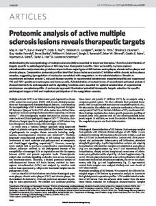
EARTH ORIENTATION PARAMETERS This section provides more details behind the brief rationale listed under Assertion 11. The EOPs define the angular rotation between the Earth Centered Earth Fixed (ECEF) ITRF and the International Celestial Reference Frame (ICRF). The EOPPs are predicted values of the EOPs used by CSPs as part of their orbit estimation algorithms. The ICRF is an inertial frame that is useful for orbital estimation. The orbital elements of the GNSS satellites are estimated in this inertial frame. Incorrect EOPPs could lead to the wrong position estimate in ITRF. In the worst case, the measurements for this incorrect position fix would all be consistent with one another and therefore not detectable by the aircraft algorithm.

Figure 1. Historic EOP values The overall organization responsible for estimating and predicting EOP values is the International Earth Rotation and Reference Frame Service (IERS) [10]. Figure 1 shows historical values from the IERS for the angular offset of Earth’s axis of rotation towards 90° W (Polar X) and towards the prime meridian (Polar Y). Also shown is the length of day (actual time taken to complete one rotation. Figure 2 shows the changes in these parameters from one day to the next. In the United States, the U.S. Naval Observatory coordinates with IERS to create and disseminate the EOPP values. These are then downloaded by the National Geospatial-Intelligence Agency (NGA) who then provides them to the Air Force for use by GPS. Each organization has its own quality and consistency checking before accepting the EOPPs. The details of these checks, the time it takes to complete an update, and the frequency of update are not publicly described. Russia has its own Institute of Applied Astronomy (IAA) that participates in the estimation of EOP values and that provides them to GLONASS. Europe has the Paris Observatory and other national observatories that participate in estimating EOPs and that can provide these values for Galileo. Finally, China also has its own national observatories to provide values for Beidou. The orbit estimation process begins with pseudorange measurements made to the satellites from terrestrial reference stations. These stations are fixed to an ECEF reference frame. If the orbits were determined instantaneously, an inertial frame would not be necessary. However, because measurements over several days may be used in the estimation process, they are combined with a dynamic model that is best represented in an inertial frame. The EOPPs are used to rotate the measurements into this frame and are then again used to rotate the satellite position estimates back out to the ECEF frame.

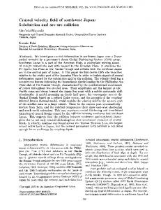
Figure 2. Historic changes in EOP values from one day to the next Erroneous EOPP values that are closely aligned to the true axis of rotation, but that have a constant offset about the axis of rotation, will have a negligible impact on the final position estimates, since the both the rotation and its inverse are used. It would take a significant misalignment of the rotation axis or an inconsistent set of rotational values (several milliseconds change to the length of day) over the course of a couple of days for bad EOPP values to create an appreciable satellite positioning error. Such errors would be much larger than historical variations. The EOPs are predictable to the centimeter level over days and to the meter level over months [11]. The solid Earth exchanges angular momentum with the atmosphere and the hydrosphere, which are the dominant sources of EOP variation. However, these variations are measured in milliarcseconds (mas), which corresponds to one thousandth of 1/3600 of one degree of rotation. One mas corresponds to a 3.1 cm horizontal shift at Earth’s surface. Incorrect EOPPs can arise from erroneous reported values or theoretically from sudden changes to the true values. However, the true EOPs do not change very quickly. Historically, the largest observed pole motion is less than 25 cm per day and the largest observed change in the length of day is under half a millisecond (also of order 25 cm) per day (see Figure 2). Thus, erroneous changes in EOPPs leading to a meter or larger effect are readily apparent and can be very effectively screened out by any GNSS Constellation Service Provider (CSP). A consistent and harmful EOPP fault common to all constellations would require a sudden EOP change well outside all historical observation or a common mode prediction error at multiple centers. This error would have to fail to be caught at multiple EOP centers and multiple CSPs. Even in such an event, the fault would

spread to satellites over an extended time scale rendering it initially observable to the airborne algorithm. The CSPs would need to continue to fail to observe the error for an extended time in order to ultimately reach the state where all satellite measurements were consistently wrong. Even in this final state, the error would be exclusively in the horizontal direction and likely small. Any EOPP error greater than 1 m should be readily observable through simple consistency checks. Thus, a multi-meter error or larger would be exceedingly unlikely to escape detection for long enough to be broadcast to multiple satellites.

These three assumptions require further discussion; if the majority of the community accepts them as true, they may be elevated to assertions. Otherwise they should be refined or replaced until there is consensus on a workable set of assertions. For now we will work with these assumptions to see what we can learn from them. Sufficiently rare events that are described by the three assumptions above are expected to follow a Poisson distribution. The probability ( | ), of observing exactly k events over interval, T, for a given rate R is ( | )=

VERIFICATION OF THE FAULT RATES Definition 1 provides a deterministic definition of a GPS fault regardless of the state of any of the other satellites. It is possible to use this fault definition to determine when faults have occurred on GPS. Such information may then be used to determine a range possible fault rates. Several assumptions are used to infer a fault rate base upon these observed faults: 1. 2. 3.

The probability of a fault occurring within a time interval is proportional to the length of that time interval, A fault occurring in one time interval does not affect the probability of it occurring in other time intervals (when the SV is set healthy), and The probability of a fault occurring does not change over time.

These assumptions are uncertain which is why they are listed as assumptions rather than assertions. Without knowing the cause of a fault or what actions were taken to restore service, it is difficult to know whether or not the fault is likely to reoccur within a short timespan. However, no GPS satellite has faulted twice in the last eight years [12] let alone twice in rapid succession. Further, operation of the constellation changes over time. New satellites are launched and old satellites are retired. Satellite designs and capabilities are changed, leading to new blocks of satellites. The master control segment software is updated and the staffing changes from year to year. It is impossible to claim that the system is truly stationary. However, all evidence points to overall GPS performance improving with time. The accuracy has improved [12], the fault rates appear to be decreasing [14] and the time to identify a fault and set the satellite unhealthy appears to be decreasing [14]. If the system truly is improving over time, assuming it is constant provides a conservative estimate of the future fault rates.

(

)

! Instead we need the probability density, ( | ), of the rate, R, given k events observed over time interval T, which can be found using Bayes Rule ( | ) ( ) ( )

( | )=

Unfortunately we know neither f(R) nor P(k). However, we can approximate them by further assuming the a priori probability of R is a uniform distribution between 0 and some Rmax. We can then find P(k) from ( )=

( | ) ( ) (

= =

)

1 ! )

( + 1, !

where + 1, is the lower incomplete gamma function. As Rmax T approaches infinity, the lower incomplete gamma function approaches the gamma function. lim

→

+ 1,

= Γ( + 1) =

!

Our desired probability density is then given by ( | )=

(

) !

We want to account for this distribution of possible values for R in our final estimate of the rate. The probability of hazardously misleading information given the possibility of a particular fault is given by P(HMI) =

(

|

)

However, since the probability of fault, Pfault, itself has a distribution, f(Pfault), then the above risk can be rewritten as (

P(HMI) =

|

)

The first term in the integral does not depend on the probability of fault and can be pulled out of the integral, leading to (

P(HMI) =

|

)

Where the integral is simply the expected value of =

=

Given the equations above, this new estimate accounts for the estimation uncertainty and satisfies the top-level integrity requirement. According to Assertions 5, 8 & 9, the probability of fault is equal to the fault rate times the mean time to notify (MTTN) the user. Therefore, the conditional distribution for fault rate may be substituted into the above equation to obtain |

( | )

=

=

|

We therefore need to find the mean conditional fault rate

|

=

(

) !

=

Γ( + 2) = = !

( +1

) !

This result provides an estimate for the fault rate and fault probability that incorporates uncertainty of the true fault rate while maintaining the integrity requirement.

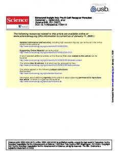
VERIFICATION OF THE WIDE FAULT RATE Let us now specifically examine the wide fault rate. We begin with GPS, which has not experienced any known constellation wide faults that would affect dual-frequency performance [12]. Figure 3 shows different values for the estimated wide fault rate, ,, = , , | , given k = 0, 1, 2, or 3 observed faults and for T between six months and ten years. As can be seen, when there are no observed faults, the expected fault rate can be set to below 10-4/hour after a little more than one year of observation.

Figure 3. Estimated wide satellite fault rate values, , , , for differing numbers of observed constellation faults. Although no faults have been observed on GPS, we may not want to have to reactively change our broadcast value of Pconst should a fault be observed subsequently. Therefore, it may be prudent to use a curve corresponding to at least one more fault than has actually been observed. By following this practice, one should wait to use the value of 10-4/hour, until at least ~2.25 years if no constellation faults are observed in that period, ~3.5 years if one constellation fault is observed, etc. Notice that it is very difficult to validate significantly smaller values of , , ∗ . It would take more than ten years to verify a value of 10-5/hour. If, as suggested above, the curve corresponding to one constellation fault is used, even though none have actually been observed, it would require more than twenty years of observation to validate that rate. For GPS, we only count the last eight years as having operated in a manner consistent enough to be treated as quasi-stationary [14]. Given eight years with no observed constellation faults, we recommend following the second line from the bottom in Figure 3. This would indicate a -5 verifiable rate for Note that the , , , of 3x10 . conservative approach makes this recommended rate twice as large as the actual expected rate. The GPS performance standard [5] does not specifically provide a wide fault rate. Instead a total fault rate per satellite is given. One can infer a wide fault rate ranging between 10-4/hour and 10-5/hour given this information. At the moment, we recommend using a wide rate of 10-4/hour for GPS combined with an MTTN of below one hour [12] to yield a value for of 10-4. If future , , specifications provide lower specified values for ,, ∗, we can consider lowering the broadcast value of , , to take advantage of this improvement, given

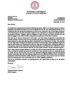
Figure 4. Estimated narrow satellite fault rate values, , , , for 30 satellites in the constellation.

Figure 5. Estimated narrow satellite fault rates, for GPS with varying averaging window lengths.

our observations. Other constellations will require at least ~2.25 years of operation with no observed constellation faults, before we could consider validating wide fault rates of 10-4/hour for them. It would be even safer to use an initial time period at least twice that length.

Figure 4 shows that the GPS spec can be validated for up to two observed faults per year with a two-year evaluation time window. However, 2.5 faults per year, on average, would require a much longer time window to validate the spec number. Multiple two-year time windows should elapse before attempting to validate rates approaching the GPS spec of 1x10-5/sat/hour. Four years would be a minimum and six years is even better. Before that period has elapsed, larger values of , , should be used that correspond to shorter time windows. It also is advisable to pad the initially observed fault count so that the estimated rate is not invalidated by subsequently occurring events.

VERIFICATION OF THE NARROW FAULT RATE The narrow fault is different from the wide fault in that multiple satellites are operating simultaneously within each constellation and the total number of faults observed is not only likely to be greater than zero, but it is also likely to increase with longer observational periods. Recently, GPS has had at least 30 healthy satellites on orbit at any given time. This means that for each hour that passes, 30 satellite-hours will be observed. We will assume that all satellites are equally likely to experience a fault (this assumption can be refined by grouping satellites by their blocks or any other suitable grouping). Under our assumptions, the observation period used for the rate estimate is the number of operational satellites multiplied by the actual time duration. Figure 4 shows a plot of the estimated narrow fault rates, given observed fault rates of between one and three observed individual faults per year. The horizontal axis is the time window used for the calculation. As an example, for one fault per year, the time window matches the number of faults, k. In one year, one fault is observed, in two years, two faults are observed, etc. For two faults per year, the number k is increased by one every six months. The estimated rates in the figure assume that there are 30 healthy satellites at any given time and that all satellites have an equal value of , , ∗.

,,

,

We next examined the estimated fault rates given the observed GPS fault history using different time windows. Five faults have been observed over the last eight years [12] (although not included in that paper, no faults were observed in 2015). Figure 5 shows the results for window lengths from six months to three years. In line with the results from Figure 4, the GPS spec rate can only be verified when the window length is two years or longer. When evaluating , , ∗ , the time window used should not be longer than one half to one third of the total evaluation period. This provides multiple independent evaluations of the fault rate. The maximum rate value obtained over the different evaluations should be used. This approach adds conservatism to the calculation and may provide evidence either for or against stationarity. For example, prior to 2011, a time window of less than one-year should have been used. A maximum value of ~2.3x10-5/sat/hour would have then been obtained. After, 2011, the one-year window would be appropriate with a corresponding maximum value of ~1.5x10-5/sat/hour. Today, in 2016, the 30-month window is appropriate with

a corresponding maximum value of ~7.6x10-6/sat/hour. As stated under Assertion 7, we will not use a rate below the specification provided by GPS. Therefore, the obtained value is sufficient to validate the specified rate -5 of , , ∗ = 1x10 /sat/hour. Combined with a MTTN of -5 one hour, we obtain a value of , , = 1x10 /sat for GPS. The above process is only conservative if the true performance improves over time. The data from 2008 – 2012 does not necessarily make it obvious that GPS performance was improving. However, the data both before 2008 and after 2012 are consistent with a general trend of improvement. If the data before 2008 is discounted, then prior to ~2014 it would have been prudent to increase the fault count used to estimate the fault rate. For example, in 2010, after observing four six month periods with at most 1 fault per any given six months, it would have been better to assume 2 faults per six months was possible. Indeed, that higher rate was observed during the next six-month period. In the first several years of operation it is best to be conservative and pad the observed fault count. For other constellations, rates approaching 1x10-5/sat/hour should only be used after there are many years with sufficiently few observed faults.

CONCLUSIONS The assertions put forward in this paper provide guidelines for offline determination of the ARAIM integrity parameters. GPS data has been previously studied to determine the observational fault rates and the αURA and bnom parameters [12]. The data indicates that the commitments described in [5] have been met. In fact, the last several years of data indicates that the commitments were very conservative relative to actual operation. However, it remains an open question how much trust to put into either the commitments or the data regarding future performance. This question is an important one for ANSPs. Those that fundamentally trust the U.S. Air Force and its operation of GPS will likely feel very confident that the historical level of performance will continue to be met going forward. Less trusting ANSPs may feel that worse behavior is possible. ARAIM should not be pursued if one cannot believe that there is a safe set of parameters that will sufficiently describe future behavior. The FAA and many other nations have trusted GPS with RAIM for many years. However many other nations have yet to approve RAIM.

The criticality of ARAIM vertical operations are more stringent than those supported by RAIM. We have provided a set of definitions and assertions to highlight the critical elements of a safety proof. This set is not yet complete. We have further demonstrated methods for validating the specified fault rates given actual observations. Our hope is to expand the discussion on these elements and ultimately foster a common international agreement on the relevant integrity parameters for each constellation. ARAIM is a very promising method for achieving global horizontal and vertical navigation. Much work remains to achieve its promise.

ACKNOWLEDGMENTS The authors would like to gratefully acknowledge the FAA Satellite Product Team for supporting this work under MOA contract number DTFAWA-15-A-80019. The opinions expressed in this paper are the authors’ and this paper does not represent a government position on the future development of ARAIM.

REFERENCES [1] Blanch, J., Walter, T., Enge, P., Wallner, S., Fernandez, F., Dellago, R., Ioannides, R., Pervan, B., Hernandez, I., Belabbas, B., Spletter, A., and Rippl, M., “Critical Elements for Multi-Constellation Advanced RAIM for Vertical Guidance,” NAVIGATION, Vol. 60, No. 1, Spring 2013, pp. 53-69. [2] Milestone 2 Report, EU-U.S. Cooperation on Satellite Navigation, Working Group-C ARAIM Technical Subgroup, February 11th, 2015. available at http://www.gps.gov/policy/cooperation/europe/2015/ working-group-c/ARAIM-milestone-2-report.pdf [3] Milestone 3 Report, EU-U.S. Cooperation on Satellite Navigation, Working Group-C ARAIM Technical Subgroup, February 26th, 2016. available at http://www.gps.gov/policy/cooperation/europe/2016/ working-group-c/ARAIM-milestone-3-report.pdf [4] “Airborne Supplemental Navigation Equipment Using the Global Positioning System (GPS),” Technical Standard Order (TSO) C-129, 10 December 1992, U.S. Federal Aviation Administration, Washington, D.C..

[5] Department of Defense, GPS Standard Positioning Service Performance Standard, 4th Edition, September 2008. [6] Walter, T., Blanch, J., and Enge, P., “Evaluation of Signal in Space Error Bounds to Support Aviation Integrity,” NAVIGATION, Journal of The Institute of Navigation, Vol. 57, No. 2, Summer 2010, pp. 101-113. [7] FAA AC 20-138B, Airworthiness Approval of Positioning and Navigation Systems, September 27, 2010. [8] RTCA, “Minimum Operational Performance Standards for Global Positioning System/ Satellite-Based Augmentation System Airborne Equipment,” DO-229D, Change 1, December, 2006. [9] FAA AC 23.1309-1E, System Safety Analysis for Part 23 Airplanes, November 17, 2011. [10] http://www.iers.org [11] Kosek, W. “Future Improvements in EOP Prediction,” in Geodesy for Planet Earth, International Association of Geodesy Symposia, Volume 136, 2012, pp 513-520. [12] Walter, T. and Blanch, J., "Characterization of GNSS Clock and Ephemeris Errors to Support ARAIM," Proceedings of the ION 2015 Pacific PNT Meeting, Honolulu, Hawaii, April 2015, pp. 920-931. [13] Whitney, S., “Global Positioning Systems Status,” Proceedings of the 28th International Technical Meeting of The Satellite Division of the Institute of Navigation (ION GNSS+ 2015), Tampa, Florida, September 2015, pp. 1193-1206. [14] Heng, L., “Safe Satellite Navigation with Multiple Constellations: Global Monitoring of GPS and GLONASS Signal-In-Space Anomalies,” Ph.D. Dissertation, Stanford University, December 2012. Available at: http://waas.stanford.edu/papers/Thesis/ LHengThesisFinalSignedSecured.pdf