If A and B are convex polyhedra then the set C = Con(A; B) is also a convex polyhedron, with points on its boundary representing con gurations which place.
Determining the Minimum Translational Distance between Two Convex Polyhedra S. A. Cameron R. K. Culley McDonnell Douglas Research Laboratories Arti cial Intelligence Technology Group St. Louis, MO, USA 63166
Abstract
Given two objects we de ne the minimal translational distance (MTD) between them to be the length of the shortest relative translation that results in the objects being in contact. MTD is equivalent to the distance between two objects if the objects are not intersecting, but MTD is also de ned for intersecting objects and it then gives a measure of penetration. We show that the computation of MTD can be recast as a con guration space problem, and describe an algorithm for computing MTD for convex polyhedra. This paper originally appeared in Int. Conf. Robotics & Automation, San Francisco, April c IEEE 1986. It was re1986, pages 591{596. formatted using LaTEX in September 1996. Cameron's address: Oxford University Computing Laboratory, Wolfson Building, Parks Road, Oxford OX1 3QD, UK. Phone: +44 1865 273850.
1 Introduction
The distance between two objects is a useful measure for reasoning about spatial relationships. However the distance between two intersecting objects is zero, which provides no information about the degree of penetration. We de ne a measure called the minimum translational distance (MTD) which overcomes this problem. Firstly, de ne the function MTD + (A; B ) as follows: MTD + (A; B ) = inf 3 f jtj : contact(A; B + t) g
t2R
where jj is the vector Euclidean length function, B + t is the result of applying the translation t to the object B (i.e. B + t = f b + t : b 2 B g), and contact(X; Y ) is true if and only if (i�) X and Y are in contact, but not overlapping. Thus MTD + is the same as the
rB
rA
d
d
Figure 1: MTD calculation for two spheres distance function for non-overlapping objects, but returns a measure of penetration for overlapping objects. MTD + is zero if the objects are in contact and positive otherwise, but does not distinguish between intersecting and non-intersecting objects. By convention, we de ne MTD itself to distinguish these cases, thus: � MTD + (A; B ) if A intersects B MTD(A; B ) = + ? MTD + (A; B ) otherwise This measure has been used to solve a collision detection problem for a robotics application [7]. As a simple example, if A and B are spheres of radius rA and rB , and their centres are distance d apart, then MTD(A; B ) = d ? rA ? rB : This special case is illustrated in Fig. 1 for two con gurations between the spheres.
2 Related work
There have been many reports of solutions to the interference detection problem | that is, given two objects say whether they intersect at some given point in time. Examples include [2, 4, 12, 13, 17]. However in all of these only a Boolean value is returned, which gives no information on the 'degree' of intersection. Comba [6] describes a 'psuedocharacteristic' function that provides some measure of the distance be-
tween convex polyhedra; he uses this to solve an interference detection problem using a numerical minimization technique. Schwartz [16] looked at the calculation of the minimum distance between convex polygons, and Cameron [4] describes an exhaustive technique for the minimum distance between arbitrary polyhedra. Recently a couple of fast solutions have been reported for calculating the minimum distance between convex polyhedra [8, 14]; these algorithms are asymptotically faster than the one reported here, but they only return zero for intersecting objects. Interest has also been shown in the calculation of distance functions in the eld of path planning. Khatib and Le Maitre [9] describe an algorithm that uses an approximate distance function, and Buckley [3] has recently reported a path-planning algorithm which is based on an optimisation method built around a proximity function, �. In fact � appears to be equal to MTD over their common range of de nition, although the two functions are de ned in di�erent ways.
space has been of interest for the formulation of path planning algorithms | for example [11, 10] | and the function Con has many nice properties. In particular we can show that for any objects A and B MTD(A; B ) = MTD(O; Con(A; B ))
(1)
where O = f 0 g is the singleton set containing the origin. To prove this note that MTD(A; B ) � 0 i� A and B overlap i� O � Con(A; B ) i� MTD(O; Con(A; B )) � 0 and so it is su�cient to show that MTD + (A; B ) = MTD + (O; Con(A; B )). If MTD + (A; B ) = d, then there exists a translation t with jtj = d such that the application of t to A will place the objects into contact. But if we interpret t as a position vector in con guration space then t must exist on the boundary of Con(A; B ), and so MTD + (O; Con(A; B )) � d. Conversely if MTD + (O; Con(A; B )) = d0 then there exists a t0 with jt0j = d0 such that t0 applied to A will put the objects into contact, and so MTD+ (A; B ) � d0. This proves the result. We have used this approach to calculate MTD for a pair of convex polyhedra, for although (1) applies in the general case, algorithms for reasoning about the con guration space obstacle are only understood for convex polyhedra.
3 Calculating MTD
The minimum distance function, dist, may be written as dist(A; B ) = inf f ja ? bj : a 2 A and b 2 B g: This suggests that to calculate dist we could simply compute the distance between every pair of points in the two objects, and take the shortest distance. For polyhedra this observation forms the basis of a practical algorithm, whereby we nd the minimum of the distances between pairs of faces, each pair consisting of a face from each object. However this does not work for MTD + , because we need to nd a pair of points such that if we translate one object to superimpose the points then the objects do not properly overlap; that is, MTD + (A; B ) = inf f ja ? bj : a 2 A and b 2 B and A \ (B + a ? b) = ; g where \ is the regularised set intersection operation [15]. This added complexity lead us to consider another approach to the problem. Given two objects their Minkowski di�erence is given by Con(A; B ) = f b ? a : a 2 A and b 2 B g This set is also called the (translational) con guration space obstacle, and it is the set of translations of A that brings it into interference with B . Con guration
4 Computing the Con guration Space Obstacle
If A and B are convex polyhedra then the set C = Con(A; B ) is also a convex polyhedron, with points on its boundary representing con gurations which place A and B into contact. Furthermore, the faces of C correspond to modes of contact of the objects such that they can slide in two independent directions, and these modes can be classi ed as: (FV) A face of A sliding against some part of B (EE) An edge of A sliding against a non-parallel edge of B (VF) Some part of A sliding against a face of B. These results are shown in [10], as is an algorithm for computing C which we call the vertex set di�erence algorithm. (The vertex set di�erence algorithm computes C by forming a set of points, each point being the vector di�erence of a vertex of A from a vertex of B , and then taking the convex hull of this new set of points.) We have implemented this algorithm, but 2
hnA ; ?dAi is a weakly necessary half-space for C. This
nA
two-dimensional case has exact analogues for the (FV) and (VF) cases in three-dimensions. For the three-dimensional case we need to nd features on one object that are extreme in the direction of the inward-pointing normal of a face of the other object. We use a winged-edge data structure for the objects [1] which makes the topological relations explicit between the vertex, edge and face features, and thus by a combination of carefully scanning the faces and hill-walking to nd the extrema we are able to nd these half-spaces in almost linear time. We also remember the single feature of the other object that can slide against each face | this information is used to generate the (EE) half-spaces. In the (EE) case not every pair of edges will generate a weakly necessary half-space. A weakly necessary half-space generated by some pair of edges must have a surface normal which is perpendicular to both edges. Thus given a pair of edges we can generate all possible supporting half-spaces (there are two pairs for each pair of edges) and check whether indeed the edges can come into contact; the edges can come into contact i� each lies in the boundary of its respective supporting half-space. This suggest a simple algorithm for computing the (EE) half-spaces which examines all pairs of edges and is thus (at least) quadratic in time. A better approach is to use the information about sliding features which is stored during the (FV) and (VF) phases; this enables us to quickly nd all the edges which can slide against a given edge. The details are given in [5].
B
A
HA
HB
dA
Figure 2: Two convex polygons and a pair of supporting half-spaces have found it too slow for our purposes; this is partly because it generates a complete boundary representation of C . Instead we have produced a faster algorithm that describes C as a list of planar half-spaces, i.e. \ C = hni; dii i
where hni; dii = f x : ni � x + di � 0 g, and each ni is a unit vector giving the outward pointing normal to the half-space boundary. We also require that each half-space be weakly necessary, where by weakly necessary we mean that for each hni ; dii in the list there exists a face of C such that the face lies in hni ; dii. (Not all the half-spaces need be strictly necessary, as it is possible for more than one half-space to correspond to a single face of C.) Given this data-structure it is possible to quickly calculate the minimum translational distance, as described in the next section. As each half-space must be weakly necessary then we only need look for half-spaces corresponding to the constraints (FV), (EE) and (VF); these are half-spaces whose boundaries lie parallel to faces of A, or parallel to a pair of edges from A and B , or parallel to faces of B . In fact each face of A and B will generate a weakly necessary half-space for C . To illustrate this, consider the situation shown in Fig. 2, in which A, B and C are convex polygons. (This is simply for clarity; the arguments apply directly to the three-dimensional case). We have shown a half-space, HA, the boundary of which passes through a 1-face (edge) of A so that A is contained in HA . HB is a half-space obtained by complementing HA and then translating it so that its boundary touches B , with HB enclosing B . We call these half-spaces supporting half-spaces. Then if nA is the unit normal to HA , some non-trivial set of translations of A of the form dA nA + pA will bring A and B into contact, where pA is perpendicular to nA and dA is the (signed) distance between HA and HB . Thus
5 Calculating the Distance to the Con guration Space Obstacle
We have as input a list of half-spaces, L = f hni; dii g, which represents C . It turns out that we can get a good estimate of the value of MTD simply by scanning this list, as follows. Assume that some df � di for all i. We want to calculate MTD, the signed distance from the origin to the boundary of C . Note that if df � 0 then for every half-space
ni � 0 + d i = d i � 0
and so the origin is in C ; conversely if df > 0 then the origin is outside hnf ; df i and is thus outside C . Furthermore, if df � 0 then the point p1 = ?df nf lies on the boundary of C , as it lies on nf � x + df = 0 and within every half-space; also any point p with jpj < jp1j must lie inside C , as
ni � p + di � jpj + di < jp1j + di � di ? df � 0:
3
So if df � 0 then df = MTD. Otherwise p1 lies on the boundary of hnf ; df i, and as C � hnf ; df i we have MTD � jp1j = df . It is then an easy matter to check whether p1 lies on C by substituting it into the half-space equations | if it does we can state that MTD = df . Thus MTD � (L) = max f di g i
arc
p
p1
origin
2
p’
L1
Po
Figure 3: Two-dimensional Example
is a good estimate for MTD, as � MTD if MTD � 0 � MTD (L) = � MTD if MTD > 0 We further hypothesis that for MTD > 0, p 3 � MTD � (L) � MTD when A and B are objects containing no edges whose surrounding faces make acute angles. (If this restriction is lifted we can generate arbitrarily bad counter examples.) Experimentally MTD � gives very good results, and is used extensively in the work reported in [7]. To nd MTD itself we hunt for a point on C which is closest to the origin. For simplicity we will rst describe the situation in two dimensions, when the halfspaces have linear boundaries in some plane and de ne a convex polygon | say Po. In this case hnf ; df i is the half-space with boundary furthest from the origin (in the positive sense), and p1 is the foot of the perpendicular from the origin to the bounding line | say the line L1. If p1 does not lie on the polygon then we look at every other half-space boundary to see where it cuts L1 , and form a list of one-dimensional half-spaces, which are the intervals that each linear half-space occupies on L1 . The intersection of these intervals gives us the boundary of the polygon on L1, and so we can nd the closest point to the origin on Po \ L1 | call this point p2. We claim that p2 must be the closest point to the origin on Po; to show this, consider Fig. 3, which shows p1 , L1 , part of Po, and an arc of a circle centred on the origin and passing through p2. If there is a closer point on Po to the origin it must exist within the intersection of the circle and hnf ; df i. Let p0 be a point in this intersection such that the line from p2 to p0 makes the smallest angle with L1 . Then by convexity there exists an edge of Po from p2 to p0, which must correspond to the boundary of a linear half-space. But this half-space is further from the origin than hnf ; df i, which is a contradiction. So p2 is the point we require. The technique described above is an example of dimensional reduction | we reduced the twodimensional problem to a searching problem in one
dimension. The three-dimensional version tries the same strategy, but sometimes fails, and then we have to recognize the failure and make allowances for it. The technique currently employed is as follows. If p1 is not a point of the polyhedra we take of slice of all the planar half-spaces that cut the plane nf � x + df = 0. This gives us a list of linear half-spaces, whose intersection describes a polygonal face of the polyhedra. (Such a face must exist by the weakly necessary condition.) We then apply the two-dimensional algorithm to try to nd the closest point on the polygon to p1. It is possible for the furthest linear half-space from p1 to not be weakly necessary (in the two-dimensional slice); if this occurs we fail to nd any edge of the polygon, we recognize the half-space as redundant, and so we can remove it from the list and try again. Given the closest point to p1 on the polygon | say p2 | then if it lies interior to an edge of the polygon it will be the closest point to the origin, and we are done. To show this, consider a slice through the origin, p1 and p2, and use the argument for the two-dimensional case; any closer point will imply the existence of a plane through the edge of the polygon and further from the origin than the half-space hnf ; df i. If p2 lies on a vertex then it is possible for an edge of C to run from p2 into a sphere, centred on the origin and passing through p2. In this case we use an exhaustive method to hunt, from p2, for the point closer to the origin. We nd all the unique half-spaces in L running through p2, but excluding hnf ; df i. Intersecting pairs of the boundaries of these half-spaces gives us a number of possible edge-directions; we follow any candidate edges leading into the sphere, and nd the required point. The above approach is not ideal in that, although it normally terminates in a reasonable time, it can occasionally take considerably longer. An alternative approach is as follows. If the point p1 is not part of the con guration space obstacle then we know that the closest point is not on a face, and so it must lie on an edge or at a vertex. We thus nd any vertex of the con guration space obstacle, and use the sliding feature information (stored with every face) to hill4
Number of runs: Number of runs with non-intersecting objects: Number of runs requiring exhaustive distance calculation: Average number of vertices per convex hull: Average CPU time for construction of halfspace lists: Average CPU time for measuring distance to the con guration space obstacle: Maximum CPU time for the entire MTD function: Average/Maximum percentage error if we calculate MTD � instead of MTD (over non-intersecting cases):
climb to the vertex which is closest to the origin. It is then easy to check whether this vertex is the closest point on the body; otherwise we need to search for the closer feature, which we hypothesize to be a nearby edge. This approach has not yet been tested experimentally, but the steps required to nd the vertices and edges of the con guration space obstacle are described in [5].
6 Testing the Algorithm
To provide evidence for the speed and e�cacy of the algorithm we tested it by using a number of pairs of random convex hulls. The values of MTD so obtained were checked in the non-overlapping cases by an exhaustive computation of the minimum distance, as in [4]. This gave us some con dence in the correctness of both stages of the algorithm, namely the construction of the half-space list and the subsequent distance calculation. For overlapping objects this test does not work; however in this case the distance calculation itself is trivial, and the construction of the con guration space obstacles is the same as for the non-overlapping cases. To generate a random convex hull we generated 100 points using a unit spherical distribution, then perturbed the radius of each point slightly (using r = 1 + R3 , where R is a uniform random variable from [-0.5, 0.5]), and then took the convex hull of this point set. This typically gave us a convex hull with about 70 vertices. One hull from each pair of hulls was left centred on the origin, but scaled along each axis using three scale factors taken uniformly from [0.5, 3], and the other was translated by a vector, each component of which was taken uniformly from [-10, 10]. (These factors were varied in other runs of the experiment, as was the seed for the pseudo-random number generator; no substantial di�erences were noticed.) In table 1 we have tabulated the statistics obtained over one run; the CPU timings are for a VAX 8600 computer. It should be noted that the convex hulls generated show less order than models of manufactured parts, but that the timings for the two classes of objects seem similar (as seen in the work described in [7]). We have not yet attempted a theoretical study of the time complexity of the algorithm; the time taken by the distance computation phase of the algorithm can occasionally be markedly higher than its norm. However, the computation of the half-space list is quite predictable for a given size of input, and has been graphed. For what it is worth, this would suggest an experimental time complexity of slightly better
100 99 56 69.7 408ms 266ms 3970ms 0.44/5.14
Table 1: Sample Measurements from the MTD function. than O(n log n), for inputs of size up to 100 vertices per hull.
7 Discussion
We have described a complete algorithm to compute the function MTD between a pair of convex hulls. The algorithm consists of two stages, namely calculation of the con guration space obstacle (CSO) as a list of planar half-spaces, followed by calculation of the minimum translational distance between the origin and the CSO. As given the algorithm is more complicated for the cases when the objects are not interfering, as the second stage can require more steps, although in practice the non-interfering case can often be dealt with faster, as heuristics may be employed to calculate the distance between two objects without computing the CSO. One such heuristic is to use hill-walking to nd a pair of vertices on the hull that are close together; this by itself does not guarantee nding the answer, but we can use these vertices to look for a pair of supporting half-planes that will tell us whether these vertices are su�cient. Another approach would be to allow preprocessing of the convex hulls for a minimum distance calculation, as in [8], and to call the MTD function only if the objects are found to be interfering. If MTD is to be calculated many times for the same pair of objects then other methods may be used to speed up the calculation. If the objects are always oriented in the same relative directions then the shape of the CSO will remain the same, and we can calculate the half-spaces once and translate them as required. If the orientations change, but the objects only move a little between iterations, then we can try saving information from one iteration to guide the search for 5
the solution of the next; however we do not know any sensible way to do this once the objects are interfering. If we only need an approximate answer to the MTD function then several techniques are known for nonintersecting objects. One technique is to use the function MTD � , and a second is to guess at a pair of supporting half-spaces for the objects and to use the distance between those. A third technique is to use enclosing approximations to the hulls, such as spheres or boxes, and this is especially appropriate if the objects are widely separated. Again no similar technique is known for the case of intersecting objects; we would imagine that it would be possible to use enclosed approximations of the objects in this case, but the advantages do not seem as obvious as those for non-intersecting objects. Our approach to the calculation of MTD can also be used for polygons, in which case the con guration space obstacle can be computed as a polygon in linear time [10], yielding a linear time algorithm for MTD.
[9] O. Khatib and J. F. le Maitre. Dynamic control of manipulators in operational space. In 3rd CISMIFToMM, pages 267{282, Udine, September 1978. [10] T. Lozano-P�erez. Spatial planning|a con guration space approach. IEEE Transactions on Computers, C-32(2):108{120, February 1983. [11] T. Lozano-P�erez and M. A. Wesley. An algorithm for planning collision-free paths among polyhedral obstacles. Communications of the ACM, 22(10):560{570, October 1979. [12] K. Maruyama. A procedure to determine intersections between polyhedral objects. Int. J. Comput. and Inf. Sci., 1(3):255{265, 1972. [13] D. E. Muller and F. P. Preparata. Finding the intersection of two convex polyhedra. Theoretical Computer Science, 7:217{236, 1978. [14] M. Orlowski. The computation of the distance between polyhedra in 3-space. SIAM. Conf. Geometric Modelling and Robotics, Albany NY, July 1985. [15] A. A. G. Requicha. Mathematical models of rigid solid objects. Technical Report PAP TM-28, University of Rochester, November 1977. [16] J. T. Schwartz. Finding the minimum distance between two convex polygons. Information Processing Letters, 13(4{5):168{170, 1981. [17] R. B. Tilove. A null-object detection algorithm for constructive solid geometry. Communications of the ACM, 27(7):684{693, July 1984.
Acknowledgement
This project owes much to the help and direction of Karl Kempf.
References
[1] B. G. Baumgart. Geometric Modelling for Computer Vision. PhD thesis, Stanford, October 1974. Reprinted as Stanford AIM-249. [2] J. W. Boyse. Interference detection among solids and surfaces. Communications of the ACM, 22(1):3{9, 1979. [3] C. E. Buckley and L. J. Leifer. A proximity metric for continuum path planning. In 9th Int. Conf. Arti cial Intelligence, pages 1096{1102, August 1985. [4] S. A. Cameron. Modelling Solids in Motion. PhD thesis, University of Edinburgh, 1984. Available from the Department of Arti cial Intelligence. [5] S. A. Cameron. An e�cient algorithm for computing the translational con guration space obstacle of two convex polyhedra. Unpublished internal memo, January 1986. [6] P. G. Comba. A procedure for detecting intersections of three-dimensional objects. J. ACM, 3:354{ 366, 1968. [7] R. K. Culley and K. G. Kempf. A collision detection algorithm based on velocity and distance bounds. In Int. Conf. Robotics & Automation, pages 1064{1069, San Francisco, April 1986. [8] D. P. Dobkin and D. G. Kirkpatrick. A linear algorithm for determining the separation of convex polyhedra. J. Algorithms, 6:381{392, 1985.
6