Determinism, Complexity, and Predictability in Computer Performance Joshua Garland∗ , Ryan G. James‡ and Elizabeth Bradley∗† of Computer Science University of Colorado, Boulder, Colorado 80309-0430 USA Email:
[email protected] † Santa Fe Institute, 1399 Hyde Park Road, Santa Fe, New Mexico 87501 USA Email:
[email protected] ‡ Complexity Sciences Center & Physics Dept., University of California, Davis, California 95616 USA Email:
[email protected]
Abstract—Computers are deterministic dynamical systems [1]. Among other things, that implies that one should be able to use deterministic forecast rules to predict their behavior. That statement is sometimes—but not always—true. The memory and processor loads of some simple programs are easy to predict, for example, but those of more-complex programs like gcc are not. The goal of this paper is to determine why that is the case. We conjecture that, in practice, complexity can effectively overwhelm the predictive power of deterministic forecast models. To explore that, we build models of a number of performance traces from different programs running on different Intel-based computers. We then calculate the permutation entropy—a temporal entropy metric that uses ordinal analysis—of those traces and correlate those values against the prediction success.
save power by putting that thread on hold for that time period (e.g., by migrating it to a processing unit whose clock speed is scaled back). Computer performance traces are, however, very complex. Even a simple “microkernel,” like a three-line loop that repeatedly initializes a matrix in columnmajor order, can produce chaotic performance traces [1], as shown in Figure 1, and chaos places fundamental limits on predictability. 4
2.3
x 10
2.25
cache misses
arXiv:1305.5408v1 [nlin.CD] 23 May 2013
∗ Dept.
2.2
2.15
I. I NTRODUCTION 2.1
Computers are among the most complex engineered artifacts in current use. Modern microprocessor chips contain multiple processing units and multi-layer memories, for instance, and they use complicated hardware/software strategies to move data and threads of computation across those resources. These features—along with all the others that go into the design of these chips— make the patterns of their processor loads and memory accesses highly complex and hard to predict. Accurate forecasts of these quantities, if one could construct them, could be used to improve computer design. If one could predict that a particular computational thread would be bogged down for the next 0.6 seconds waiting for data from main memory, for instance, one could
2.05
7.742
7.743
7.744
7.745
7.746
7.747
7.748
time (instructions x 100,000)
7.749
7.75
7.751 4
x 10
Fig. 1. A small snippet of the L2 cache miss rate of col_major, a three-line C program that repeatedly initializes a matrix in column-major order, running on an Intel Core R Duo -based machine. Even this simple program exhibits chaotic performance dynamics.
The computer systems community has applied a variety of prediction strategies to traces like this, most of which employ regression. An appealing alternative builds on the recently established fact that computers can be effectively modeled as deterministic nonlinear dynamical systems [1]. This result implies the existence of a deterministic forecast rule for those dynamics. In particular, one can
II. M ODELING C OMPUTER P ERFORMANCE Delay-coordinate embedding allows one to reconstruct a system’s full state-space dynamics from a single scalar time-series measurement— provided that some conditions hold regarding that data. Specifically, if the underlying dynamics and the measurement function—the mapping from ~ to the scalar value the unknown state vector X x that one is measuring—are both smooth and generic, Takens [4] formally proves that the delaycoordinate map F (τ, m)(x) = ([x(t) x(t + τ ) . . . x(t + mτ )])
cache misses (t + 2τ)
use delay-coordinate embedding to reconstruct the underlying dynamics of computer performance, then use the resulting model to forecast the future values of computer performance metrics such as memory or processor loads [2]. In the case of simple microkernels like the one that produced the trace in Figure 1, this deterministic modeling and forecast strategy works very well. In morecomplicated programs, however, such as speech recognition software or compilers, this forecast strategy—as well as the traditional methods— break down quickly. This paper is a first step in understanding when, why, and how deterministic forecast strategies fail when they are applied to deterministic systems. We focus here on the specific example of computer performance. We conjecture that the complexity of traces from these systems—which results from the inherent dimension, nonlinearity, and nonstationarity of the dynamics, as well as from measurement issues like noise, aggregation, and finite data length—can make those deterministic signals effectively unpredictable. We argue that permutation entropy [3], a method for measuring the entropy of a real-valued-finite-length time series through ordinal analysis, is an effective way to explore that conjecture. We study four examples—two simple microkernels and two complex programs from the SPEC benchmark suite—running on different Intel-based machines. For each program, we calculate the permutation entropy of the processor load (instructions per cycle) and memory-use efficiency (cache-miss rates), then compare that to the prediction accuracy attainable for that trace using a simple deterministic model.
4
x 10 2.35 2.3 2.25 2.2 2.15 2.35
2.3 2.25 2.2 4
x 10
2.15 2.1 2.05
cache misses (t + τ)
2.05
2.1
2.15
2.2
2.25
2.35
2.3 4
x 10
cache misses (t)
Fig. 2. A 3D projection of a delay-coordinate embedding of the trace from Figure 1 with a delay (τ ) of 100,000 instructions.
from a d-dimensional smooth compact manifold M to Re2d+1 , where t is time, is a diffeomorphism on M —in other words, that the reconstructed dynamics and the true (hidden) dynamics have the same topology. This is an extremely powerful result: among other things, it means that one can build a formal model of the full system dynamics without measuring (or even knowing) every one of its state variables. This is the foundation of the modeling approach that is used in this paper. The first step in the process is to estimate values for the two free parameters in the delay-coordinate map: the delay τ and the dimension m. We follow standard procedures for this, choosing the first minimum in the average mutual information as an estimate of τ [5] and using the false-near(est) neighbor method of [6], with a threshold of 10%, to estimate m. A plot of the data from Figure 1, embedded following this procedure, is shown in Figure 2. The coordinates of each point on this plot are differently delayed elements of the col_major L2 cache miss rate time series y(t): that is, y(t) on the first axis, y(t + τ ) on the second, y(t + 2τ ) on the third, and so on. Structure in these kinds of plots—clearly visible in Figure 2—is an indication of determinism1 . That structure can also be used to build a forecast model. Given a nonlinear model of a deterministic dynamical system in the form of a delay-coordinate embedding like Figure 2, one can build deterministic forecast algorithms by capturing and exploiting the geometry of the embedding. Many 1 A deeper analysis of Figure 2—as alluded to on the previous page—supports that diagnosis, confirming the presence of a chaotic attractor in these cache-miss dynamics, with largest Lyapunov exponent λ1 = 8000 ± 200 instructions, embedded in a 12-dimensional reconstruction space [1].
techniques have been developed by the dynamical systems community for this purpose (e.g., [7], [8]). Perhaps the most straightforward is the “Lorenz method of analogues” (LMA), which is essentially nearest-neighbor prediction in the embedded state space [9]. Even this simple algorithm—which builds predictions by finding the nearest neighbor in the embedded space of the given point, then taking that neighbor’s path as the forecast—works quite well on the trace in Figure 1, as shown in Figure 3. On the other hand, if we use the same 4
x 10
col_major cache misses
2.35
2.3
2.25
2.2
2.15
2.1
2.05 82,125
82,625
83,125
83,625
84,125
84,625
time (instructions x 100,000)
85,125
85,625
86,125
Table I presents detailed results about the prediction accuracy of this algorithm on four different examples: the col_major and 482.sphinx3 programs in Figures 3 and 4, as well as another simple microkernel that initializes the same matrix as col_major, but in row-major order, and another complex program (403.gcc) from the SPEC cpu2006 benchmark suite. Both microkerR nels were run on the Intel Core Duo machine; R both SPEC benchmarks were run on the Intel i7 machine. We calculated a figure of merit for each prediction as follows. We held back the last k elements3 of the N points in each measured time series, built the forecast model by embedding the first N − k points, used that embedding and the LMA method to predict the next k points, then computed the Root Mean Squared Error (RMSE) between the true and predicted signals: s Pk 2 i=1 (ci − pˆi ) RM SE = k
Fig. 3. A forecast of the last 4,000 points of the signal in Figure 1 using an LMA-based strategy on the embedding in Figure 2. Red circles and blue ×s are the true and predicted values, respectively; vertical bars show where these values differ.
To compare the success of predictions across signals with different units, we normalized RMSE as follows: RM SE nRM SE = Xmax,obs − Xmin,obs
approach to forecast the processor load2 of the 482.sphinx3 program from the SPEC cpu2006 R benchmark suite, running on an Intel i7 -based machine, the prediction is far less accurate; see Figure 4.
TABLE I N ORMALIZED ROOT MEAN SQUARED ERROR ( N RMSE) OF 4000- POINT PREDICTIONS OF MEMORY & PROCESSOR PERFORMANCE FROM DIFFERENT PROGRAMS . cache miss rate
instrs per cycle
row_major
0.0324
0.0778
col_major
0.0080
0.0161
403.gcc
0.1416
0.2033
482.sphinx3
0.2032
0.3670
3
482.sphinx3 IPC
2.5
2
1.5
1
0.5
0 62,137
62,637
63,137
63,637
64,137
64,637
time (instructions x 100,000)
65,137
65,637
66,137
Fig. 4. An LMA-based forecast of the last 4,000 points of a processor-load performance trace from the 482.sphinx3 benchmark. Red circles and blue ×s are the true and predicted values, respectively; vertical bars show where these values differ. 2 Instructions
per cycle, or IPC
The results in Table I show a clear distinction between the two microkernels, whose future behavior can be predicted effectively using this simple deterministic modeling strategy, and the more-complex SPEC benchmarks, for which this prediction strategy does not work nearly as well. This begs the question: If these traces all come from deterministic systems—computers— then why are they not equally predictable? Our 3 Several different prediction horizons were analyzed in our experiment; the results reported in this paper are for k=4000
conjecture is that the sheer complexity of the dynamics of the SPEC benchmarks running on the R Intel i7 machine make them effectively impossible to predict.
ordinal pattern, φ(x1 , x2 , x3 ), is 231 since x2 ≤ x3 ≤ x1 . This method has many features; among other things, it is robust to noise and requires no knowledge of the underlying mechanisms.
III. M EASURING C OMPLEXITY
Definition (Permutation Entropy). Given a time series {xt }t=1,...,T . Define Sn as all n! permutations π of order n. For each π ∈ Sn we determine the relative frequency of that permutation occurring in {xt }t=1,...,T :
For the purposes of this paper, one can view entropy as a measure of complexity and predictability in a time series. A high-entropy time series is almost completely unpredictable—and conversely. This can be made more rigorous: Pesin’s relation [10] states that in chaotic dynamical systems, the Shannon entropy rate is equal to the sum of the positive Lyapunov exponents, λi . The Lyapunov exponents directly quantify the rate at which nearby states of the system will diverge with time: |∆x(t)| ≈ eλt |∆x(0)|. The faster the divergence, the more difficult prediction becomes. Utilizing entropy as a measure of temporal complexity is by no means a new idea [11], [12]. Its effective usage requires categorical data: xt ∈ S for some finite or countably infinite alphabet S, and data taken from real-world systems is effectively real-valued. To get around this, one must discretize the data—typically by binning. Unfortunately, this is rarely a good solution to the problem, as the binning of the values introduces an additional dynamic on top of the intrinsic dynamics whose entropy is desired. The field of symbolic dynamics studies how to discretize a time series in such a way that the intrinsic behavior is not perverted, but these methods are fragile in the face of noise and require further understanding of the underlying system, which defeats the purpose of measuring the entropy in the first place. Bandt and Pompe introduced permutation entropy (PE) as a “natural complexity measure for time series” [3]. Permutation entropy employs a method of discretizing real-valued time series that follows the intrinsic behavior of the system under examination. Rather than looking at the statistics of sequences of values, as is done when computing the Shannon entropy, permutation entropy looks at the statistics of the orderings of sequences of values using ordinal analysis. Ordinal analysis of a time series is the process of mapping successive time-ordered elements of a time series to their value-ordered permutation of the same size. By way of example, if (x1 , x2 , x3 ) = (9, 1, 7) then its
p(π) =
|{t|t ≤ T − n, φ(xt+1 , . . . , xt+n ) = π}| T −n+1
Where | · | is set cardinality. The permutation entropy of order n ≥ 2 is defined as X p(π) log2 p(π) H(n) = − π∈Sn
Notice that 0 ≤ H(n) ≤ log2 (n!) [3]. With this in mind, it is common in the literature to normalize H(n) permutation entropy as follows: log . With this 2 (n!) convention, “low” entropy is close to 0 and “high” entropy is close to 1. Finally, it should be noted that the permutation entropy has been shown to be identical to the Shannon entropy for many large classes of systems [13]. In practice, calculating permutation entropy involves choosing a good value for the wordlength n. The key consideration here is that the value be large enough that forbidden ordinals are discovered, yet small enough that reasonable statistics over the ordinals are gathered: e.g., n = argmax{T > 100`!}, assuming an average of 100 `
counts per ordinal. In the literature, 3 ≤ n ≤ 6 is a standard choice—generally without any formal justification. In theory, the permutation entropy should reach an asymptote with increasing n, but that requires an arbitrarily long time series. In practice, what one should do is calculate the persistent permutation entropy by increasing n until the result converges, but data length issues can intrude before that convergence is reached. Table II shows the permutation entropy results for the examples considered in this paper, with the nRMSPE prediction accuracies from the previous section included alongside for easy comparison. The relationship between prediction accuracy and the permutation entropy (PE) is as we conjectured: performance traces with high PE—those
TABLE II P REDICTION ERROR ( IN N RMSPE) AND PERMUTATION ENTROPY ( FOR DIFFERENT WORDLENGTHS n cache misses row_major col_major 403.gcc 482.sphinx3 insts per cyc row_major col_major 403.gcc 482.sphinx3
error 0.0324 0.0080 0.1416 0.2032 error 0.0778 0.0161 0.2033 0.3670
n=4 0.6751 0.5029 0.9916 0.9913 n=4 0.9723 0.8356 0.9862 0.9951
n=5 0.5458 0.4515 0.9880 0.9866 n=5 0.9354 0.7601 0.9814 0.9914
n=6 0.4491 0.3955 0.9835 0.9802 n=6 0.8876 0.6880 0.9764 0.9849
whose temporal complexity is high, in the sense that little information is being propagated forward in time—are indeed harder to predict using the simple deterministic forecast model described in the previous section. The effects of changing n are also interesting: using a longer wordlength generally lowers the PE—a natural consequence of finite-length data—but the falloff is less rapid in some traces than in others, suggesting that those values are closer to the theoretical asymptote that exists for perfect data. The persistent PE values of 0.5–0.6 for the row_major and col_major cache-miss traces are consistent with dynamical chaos, further corroborating the results of [1]. (PE values above 0.97 are consistent with white noise.) Interestingly, the processor-load traces for these two microkernels exhibit more temporal complexity than the cache-miss traces. This may be a consequence of the lower baseline value of this time series. IV. C ONCLUSIONS & F UTURE W ORK The results presented here suggest that permutation entropy—a ordinal calculation of forward information transfer in a time series—is an effective metric for predictability of computer performance traces. Experimentally, traces with a persistent PE ' 0.97 have a natural level of complexity that may overshadow the inherent determinism in the system dynamics, whereas traces with PE / 0.7 seem to be highly predictable (viz., at least an order of magnitude improvement in nRMSPE). If information is the limit, then gathering and using more information is an obvious next step. There is an equally obvious tension here between data length and prediction speed: a forecast that
requires half a second to compute is not useful for the purposes of real-time control of a computer system with a MHz clock rate. Another alternative is to sample several system variables simultaneously and build multivariate delay-coordinate embeddings. Existing approaches to that are computationally prohibitive [14]. We are working on alternative methods that sidestep that complexity. ACKNOWLEDGMENT This work was partially supported by NSF grant #CMMI-1245947 and ARO grant #W911NF-121-0288. R EFERENCES [1] T. Myktowicz, A. Diwan, and E. Bradley, “Computers are dynamical systems,” Chaos, vol. 19, p. 033124, 2009, doi:10.1063/1.3187791. [2] J. Garland and E. Bradley, “Predicting computer performance dynamics,” in Proceedings of the 10th International Conference on Advances in Intelligent Data Analysis X, Berlin, Heidelberg, 2011, pp. 173–184. [3] C. Bandt and B. Pompe, “Permutation entropy: A natural complexity measure for time series,” Phys Rev Lett, vol. 88, no. 17, p. 174102, 2002. [4] F. Takens, “Detecting strange attractors in fluid turbulence,” in Dynamical Systems and Turbulence, D. Rand and L.-S. Young, Eds. Berlin: Springer, 1981, pp. 366– 381. [5] A. Fraser and H. Swinney, “Independent coordinates for strange attractors from mutual information,” Physical Review A, vol. 33, no. 2, pp. 1134–1140, 1986. [6] M. B. Kennel, R. Brown, and H. D. I. Abarbanel, “Determining minimum embedding dimension using a geometrical construction,” Physical Review A, vol. 45, pp. 3403–3411, 1992. [7] M. Casdagli and S. Eubank, Eds., Nonlinear Modeling and Forecasting. Addison Wesley, 1992. [8] A. Weigend and N. Gershenfeld, Eds., Time Series Prediction: Forecasting the Future and Understanding the Past. Santa Fe Institute, 1993. [9] E. N. Lorenz, “Atmospheric predictability as revealed by naturally occurring analogues,” Journal of the Atmospheric Sciences, vol. 26, pp. 636–646, 1969. [10] Y. B. Pesin, “Characteristic Lyapunov exponents and smooth ergodic theory,” Russian Mathematical Surveys, vol. 32, no. 4, p. 55, 1977. [11] C. E. Shannon, “Prediction and entropy of printed English,” Bell Systems Technical Journal, vol. 30, pp. 50– 64, 1951. [12] R. Mantegna, S. Buldyrev, A. Goldberger, S. Havlin, C. Peng, M. Simons, and H. Stanley, “Linguistic features of noncoding DNA sequences,” Physical review letters, vol. 73, no. 23, pp. 3169–3172, 1994. [13] J. Amig´o, Permutation Complexity in Dynamical Systems: Ordinal Patterns, Permutation Entropy and All That. Springer, 2012. [14] L. Cao, A. Mees, and K. Judd, “Dynamics from multivariate time series,” Physica D, vol. 121, pp. 75–88, 1998.