As weil, it is wise to start iterating at a number of different initiai values and then average ...... [2] Kathleen T. Alligood, Tim D. Sauer, James A. Yorke. Chaos: an ...
DETERMINISTIC CHAOS FOR AUTHENTICATION AND SECURE COMMUNICATION
A Thesis Presented t o The Faculty of Graduate Studies
of
The University of Guelph
by
STEVEN E. SLADEWSKI
In partial fulfillrnent of requirements for the degree of -Master of Science August, 2001
@ Steven E. Sladewski, 2001
I*m
National Library of Canada
Bibliothèque nationale du Canada
Acquisitions and Bibliographie Services
Acquisitions et services bibliographiques
395 Wellington Street Ottawa O N K IA ON4
395, rue Wellington Ottawa ON Ki A ON4 Canada
Canada
Yow Me Votre rdWrance
Our file Notre ret6rence
The author has granted a nonexclusive licence allowing the National Library of Canada to reproduce, Ioan, disûibute or seli copies of this thesis in microfom? paper or electronic formats.
The author retains ownership of the copyright in this thesis. Neither the thesis nor substantial extracts from it may be p ~ t e or d otherwise reproduced without the author's permission.
L'auteur a accordé une licence non exclusive permettant à la Bibliothèque nationale du Canada de reproduire, prêter, distribuer ou vendre des copies de cette thèse sous la forme de microfiche/film, de reproduction sur papier ou sur format électronique. L'auteur conserve la propriété du droit d'auteur qui protège cette thèse. Ni la thèse ni des extraits substantiels de celle-ci ne doivent être imprimés ou autrement reproduits sans son autorisation.
ABSTRACT
DETERMINISTIC CHAOS FOR AUTHENTICATION AND SECURE COMMUNICATION
Steven E. Sladewski University of Guelph, 2001
Advisor: Professor W. F. Langford
Surprisingly, two identical or nearly identical chaotic dynamical systems can be made to synchronize. This synchronization property has been proposed as a vehicle for "secure communication". Unfortunately chaotically secured communication bas shown itself to be vulnerable to a number of decoding techniques, some of which are discussed here. Au t hentication devices send continuous signals t hat uniquely identify themselves to a receiver. Such signals must be aperiodic and sufficiently %ndorn'' that it is virtually impossible for an eavesdropper to duplicate them. In this thesis, modular arithmetic is used as an alternative number system. Using nonlinear time series analysis, the incomplete modular representation of a chaotic process is shown to be highly resistant to decoding. In this thesis we present original schemes for communication systems and authentication devices which are expected to provide a heightened measure of security.
ACKNOWLEDGEMENTS
1 would like to thaak my advisor, Dr. William Langford, for his guidance and support during the years of my graduate study. He has been of inestimable help in forrnulating my understanding of dynamical systems. 1would also like to acknowledge Dr. Heinz Bauschke, Dr. Brian Allen, and my advisory cornmittee, Dr. Pal Fischer and Dr. Anna Lawniczak, for reading this thesis and providing their invaluable advice. I would also like to thank the Department of Mathematics and Statistics for its financial support dunng my tenure as a graduate student.
Contents 1 Introduction
1
2 Determinist ic Chaos and Synchronization
4
2.1
Chaos . . . . . . . . . . . . . . . . . . . . . . . . . . . . . . . . . . .
4
2.2
Lyapunov Nurnbers and Exponents . . . . . . . . . . . . . . . . . . .
5
2.3
Lyapunov Exponents from Time Series . . . . . . . . . . . . . . . . .
9
2.4 Synchronizing Chaos . . . . . . . . . . . . . . . . . . . . . . . . . . .
12
3 Chaotically Secured Communication
17
3.1
Signal Masking . . . . . . . . . . . . . . . . . . . . . . . . . . . . . .
17
3.2
ChaoticSwitching . . . . . . . . . . . . . . . . . . . . . . . . . . . . .
19
3.3
Chaotic Modulation . . . . . . . . . . . . . . . . . . . . . . . . . . . .
20
4 Unmasking Chaotic Communication
23
5 Modular Arithmetic
31
5.1 Review of Modular Arithmetic . . . . . . . . . . . . . . . . . . . . . .
32
...............
39
5.3 Tests for Randomness . . . . . . . . . . . . . . . . . . . . . . . . . . .
43
5.4 A New Synchronization Scheme . . . . . . . . . . . . . . . . . . . . .
45
5.2 Chaotic Dynamics in Modular Arithmetic
6 Time Series Andysis
6.1 Forecasting the Future . . . . . . . . . . . . . . . . . . . . . . . . . .
48
49
Liïnitations to Nonlinear Forecasting . . . . . . . . . . . . . . . . . .
55
6.3 Determinism versus Stochasticism . . . . . . . . . . . . . . . . . . . .
59
6.2
7 Conclusions
63
A Computer Programs
70
Chapter 1 Introduction A surprising fact about chaotic dynamical systems is their ability to synchronize. Since very sensitive dependence on initia.1conditions is an essent i d characteristic of chaos, such a synchronization hardly seelus possible. Under certain circumstances, however, two or more dynamical systems which are coupled together undergo dosely related motion, even when their motions are chaotic. Here we will consider how identical, or almost identical, chaotic systems can be synchronized by a chaotic reference signal so that the two systems follow identical, or almost identical, chaotic orbits. A basic background for understanding deterministic chaos and synchronization is given in Chapter 2.
A proposed application of the ability to synchronize chaotic systems is secure communication. The sender uses the information-containing signal to modulate the chaotic signal, thus concealing the information in the signal fiom any third party who intercepts it. Then the information can be extracted by someone who possesses an exact replica synchronized to the reference signal. Because of the dificulty in predicting chaos it was surmised that such communications systerns would have a high degree of security. It was soon shown that this was not the case. Using techniques
CNAPTER 1. INTRODUCTION
2
based on a number of methods such as nonlinear forecasting, return maps, neural networks, and spectral analysis, several mathematicians were able to extract the information signal from the transmit ted signal. Chapter 3 of this thesis describes three different proposals for chaotically secured communication, and Chapter 4 explains how each was unmasked.
WhiIe a great deal of research has been devoted to using synchronized chaos for communicating an information signal, there has been Iittle interest in the problem of authenticating a chaotic signal. A typical authentication problem occurs in the design of a security system where the transmitter emits a steady stream of data (an electronic fingerprint) which uniquely identifies itself to the receiver making it practically impossible for an imposter to pose as a legitimate transmitting device. The transmitter's constant signal reassures the receiver that everything is as it should be. If the signal should be interrupted then the receiver sounds an alarm and takes whatever steps are necessary.
In a system such as this, a principal concern is duplication. Should a transmitter somehow fa11 into the wrong bands, we must be sure that the integrity of the other transmit ters is not compromised. Another concern is whether an eavesdropper could somehow monitor the signal for a long enough period of time to "clone" the monitored signal, and then substitute this clone for the actual one. An original proposa1 for an authentication scheme is presented in Chapter 3. Probably the biggest threat to the security of a communication system or an authentication system is nonlinear time series analysis. Using a method called time delay embedding, nonlinear time series analysis is able to reconstruct phase space, to model, to approximate Lyapunov exponents, and to forecast the future outcorne of a deterministic series. It is this last ability, to forecast the future, that makes "chaotically secured communication" vulnerable to attack. Whether we need an algorithm
CHAPTER 1. INTRODUCTION
3
for communication or authentication, we must be sure that the scheme is immune to nonlinear forecast ing. Nonlinear forecasting t ethniques are reviewed in Chapt ers 4 and 6. One way to foi1 attack by nonlinear forecasting is to use "modular arithmetic". Modular arithmetic is a number systern that makes use of several relatively prime
. number in this number system is represented in the moduli mi, mz,. . . ,m ~ Each form u
G
(ul, U?,. .. , U N ) where ui = u mod mi.As is shown in this thesis, represent-
ing a chaotic signal in modular f o m makes it much more difficult for an eavesdropper to extract an information signal from a transmitted signal or to predict the data stream of an authentication device. A review of modular arithmetic and novel applications of modular arithmetic for authenticating a chaotic sigrial and for chaotic communications are presented in Chapter 5 .
The main contributions of this thesis are a computational method for defining chaotic maps over the integers permitting arbitrarily long periods; a transformation that obscures the geometry of a chaotic attractor making analysis by spectral methods, return maps, and nonlinear forecast ing virtually impossible; and an original scheme for authentication and chaotically secured communication and that is robust in its resistance to unmasking.
Chapter 2 Deterministic Chaos and Synchronization 2.1
Chaos
For generations, students of the sciences learned their craft from textbooks filled with examples of differential equations with regular solutions. If these solutions remained in a bounded region of space, then they settled into one of two types of behavior, a steady state, or an oscillation that was either periodic or quasiperiodic. In the mid1970's, scientists around the world becarne aware of a third type of behavior which we cal1 chaos.
In the present day, deterministic chaos can be observed in experiments and in computer models from al1 fields of science. A key requirement for a dynarnical system to exhibit chaotic behavior is that the system must involve a nonlinearity. It is now common for an experiment whose anomalous behavior was previously explained in terms of experimental error and noise to be reevaluated for an explanation in terms of chaos.
CHAPTER 2. DETERMINISTIC CHAOS AND SYNCHRONIZATION Another key requirernent for chaos is the property of sensitive dependence on initial conditions. If we have two arbitrarily close but distinct initial points, the local behavior of the trajectories passing through these two initial points displays an exponentid growt h in the distance between these trajectories with increasing time. These two trajectories, however, do not continue to separate forever. Nonlinearity in the system causes the trajectories to fold back and remain in a bounded region of space for al1 time. The "local stretching" is essentially linear and the "global folding" is essentially nonlinear.
A better name for this type of behavior is "deterministic chaos". It is "deterministic" because the soIution of a differential equation fgr given initial conditions is uniquely determined throughout its interval of existence under the conditions of the Fundamental Existence and Uniqueness Theorem. Yet it appears to be "chaotic" in that it never repeats itself and is impossible to predict very far into the future. This paradox of the apparent coexistence of determinisrn and chaos is what rnakes chaotic dynmical systems so intriguing. For a good introduction to the theory of chaos in dynamical systems see "Chaos: An Introduction to Dynamical Systems" by Alligood, Sauer, and Yorke [Z], "An Introduction to Chaotic Dynamical Systems" by Devaney [8], or "Nonlinear Dynamics and Chaos : with Applications in Physics, Biology, Chemistry, and Engineering" by Strogatz [33].
2.2
Lyapunov Numbers and Exponents
Lyapunov numbers and exponents are useful qualitative tools for the study of chaotic systems. Suppose that f is a diffeomorphism which defines a dynamical system defined on Rm. The Lyapunov exponents Xj, j = 1,2, . . . , m, of an attractor provide a measure of the average change in distance, in orthogonal directions, of two nearby
CHAPTER 2- DETERMINISTIC CHAOS AND SYNCHRONIZATION
6
points on the attractor wïth each iteration. In other words, the Lyapunov exponents characterize the ''local stretching" mentioned above. By convention XI 2 X2 2 ,A
2
. 2
o.
Let S be a sphere of small radius
E
centered at the first point vo of an orbit.
The image f (S)of the small sphere is approximately ellipsoidal, with long axes along expanding directions and short axes along contracting ones. The per-iterate changes in the axes of our ellipsoid are essentially the Lyapunov nurnbers. To make things precise replace the sphere S with the unit sphere U centered at vo and the map f with the Jacobian matrix Df (vo). Let J, = Dfn(vo)denote the Jacobian matrix of the n-th iterate of f . Then J,U will be an ellipsoid with m orthogonal axes. The m average multiplicative expansion rates of the rn orthogonal axes are the Lyapunov numbers. We have the following definition: Definition 2.1
.
Let f be a smooth m a p o n IRm, let J, = Dfn(vo), let U be the
unit sphere centered at vo, and for k = 1,. . . ,m let r," be the length of the k-th longest orthogonal axis of the ellipsoid JnU for a n orbit with initial point vo . T h e n T,"
measures t h e contraction o r expansion along axis k near the orbit of vo during the
first n iterations. T h e k-th Lyapunov number of vo zs defined by Lk = lim,,-
(r:)'/"
provzded this Zimit exists. T h e k-th Lyapunov exponent is defined b y X k = In Lk.
If U is the unit sphere in IEg" and A is an m x m matrix, then the orthogonal axes of the ellipsoid A U may be determined in a straightforward way. The lengths of the
axes are the square roots of the eigenvalues of the covariance matrix ATA, and the axis directions are given by the m corresponding orthonormal eigenvectors of AT^.
In general, there is no explicit way to deteimine the Lyapunov numbers from knowledge of a map and its Jacobian matrùc. Since the matrix J, = Dfn(vo) is difficult to determine exactly for large n we must approximate the image ellipsoid
CHAPTER 2- DETERMEVISTIC CHAOS AND SY~VCHROLVIZATZON J,U numerically. A direct approach to calculation of the Lyapunov numbers is to form J ~ J ,and find the eigenvalues si. If the ellipsoid contains stretching and shrinking directions, it becomes long and thin. Hence, the eigenvalues of
JZJ,
include very large and very
small numbers making computations difficult.
An indirect approach described in Alligood, Sauer, and Yorke [Z]is to measure the change of the ellipsoid with each iteration. Since
we can start with an orthonormal basis {wy, . . . ,wk) for Rm. Next we compute the vect ors
z i = Df (vo)wy
While these vectors lie on the ellipse Df (vo) U they are not necessarily orthogonal. By means of the Gram-Schmidt orthogonalization process we can construct an orthogonal basis L
Y: = 21
The vectors {y:, . . . ,y ; }
span an ellipsoid of the same volume as Df (vo)Uand their
lengths are a measure of the stretch applied to the unit sphere hy the map. We next
CHAPTER 2. DETERMINISTIC CHAOS AND SYNCHRONIZATIOhT form a new orthonormal basis
Continuing in likewise fashi~nwe c m approximate the i-th Lyapunov number by
and the i-th Lyapunov exponent by
Using the above we can make the following definition.
Definition 2.2
.
Let f be a m a p of IRm, rn 2 1, and let {vu,y ,v2, . . . } be a bounded
orbit o f f . The orbit i s said to be chaotic if t h e following conditions hold: 1. It is n o t asymptotically periodic.
2. No Lyapunov number i s exactly one.
3. Ll(vo)> 1. It is important to remember that Lyapunov numbers are uniquely determined by a specific orbit. To speak of the Lyapunov numbers of a chaotic attractor for a given map, we are making the assumption that the orbit whose Lyapunov numbers we have
CHjlPTER 2, DETERWILVISTIC CHAOS AND SYlVCHRONIZATION
9
calculated is sornehow representative of the invariant set. In fact, most of the chaotic attractors which have been studied are filled with dense orbits. While the above method applies only to maps, with a littie bit of work it c m also be used to find the Lyapunov exponents of a fiow. By using a "differential equation solver" such as Runge-Kutta, we can discretize the fiow so that it has the properties cf a map.
In applying the Alligood, Sauer, and Yorke algorithrn, it is important to iterate for several thousand steps to ensure that we are on the attractor. Taking the most recent point to be the initial point for the algorithm we discard the previous output. Many thousand of further iterations of the algorithm are needed to eliminate transient behavior. As weil, it is wise to start iterating at a number of different initiai values and then average the results.
2.3
Lyapunov Exponents from Time Series
In applied science, experimental data often takes the form of a time series. Once again, probably the single most important quantitative measure of a dynamical system is the set of Lyapunov exponents. Hence, it is of great value to have a method of determining their values frorn the entries of a tirne series. One such met hod is provided by Eckmann et al. [IO]. A sumrnary of their method follows. First we choose an embedding dimension d~ and constmct a dE-dimensional orbit by means of the time-delay method. We define
where the xi are the entries of the time senes for i = 1,2, . . . ,N - d E
+ 1. Next we
CHAPTER 2. DETER7MINISTIC CHAOS AND SYNCHRONIZATION determine the neighbors of xi, namely, the points
xj
10
of the orbit which are contained
in a bal1 of suitable radius r centered at xi,
Having embedded the dynarnicd system in d E dimensions (it would be more
, next want correct to Say that we have projected the dynamical system to l R d ~ ) we to determine a d E x d E matrix T iwhich describes how the time evolution sends small vectors around xi to small vectors around xi+l. The matrix Ti is obtained by choosing neighbors
xj
of xi and imposing
~ in T ibeing only It 'S quite possible that the vectors xj - xi will not span R d resulting partially deterrnined. While this indeteminacy will not affect the calculation of the positive Lyapunov exp onents, nevertheless, it introduces spurious exponents which confuse the analysis, in particular with respect to zero or negative exponents which might be otherwise recoverable from the data. The solution to this difficulty is to allow
Ti t o be a d M x dhf matrix with d M 5 d E , corresponding to the time evolution fiom
xi to xi+,.
We may think of d M as a "local dimension" which is equal to the number
of Lyapunov exponents and is the dimension of the Jacobian matrix. Similarly d E is a "global dimension" which is used in the process of identifying neighbors and is chosen large enough to ensure that we have an embedding. Specifically, we assume that there is an integer m
2 1 such that
CHAPTER
2. DETEfiMINISTIC CHAOS AhTDSYLVCHRONEATION
11
and associate with each xi a dM-dimensional vector
in which some of the intermediate components of (2.7) have been dropped. For m > 1 we replace (2.9) by the condition
Taking rn > 1 does not mean that points are deleted from the data file. Al1 points are still acceptable as xi, and the distances are still based on d E , not on d ~ In. view of the above the matrix Tihas the rational normal form
If we define by SF(r) the set of indices j of the neighbors xj within distance r, then Ive may obtain the
ak
by a least-squares fit
Note that this algorithm will fail if card S ~ ( T 0, and s ( t ) is the received drive signal. When
s ( t ) is equal to the transmitter signal x, state variables 2 , 8, and Z will asyrnptotically
synchronize to x, y, and z, respectively, as shown in Chapter 2. The use of a transmitter-receiver pair for signal masking depends on the ability of the receiver signal z ( t ) to approximately synchronize to the transmit ter signal x ( t ) when a perturbation m(t)is added to x(t) , i.e., when s ( t ) is given by
where m(t)is the desired message to be transmitted and recovered. Since the information signal is combined with the chaotic output of the transrnitter it would seern to be very difficult, if not impossible, for an independent observer to extract the information from the transmitted signal. For the intended receiver, in posessior of system (3.2) the recovered message is
CHAPTER 3. CHAOTICALLY SECURED COMMU1VICATION with the corresponding error term of
ez ( t )= x ( t )- z ( t ).
It is necessary that this error be srnall compared to m(t). This is shown to be true in Kocarev et al. [22].
3.2
Chaotic Switching
In this method, introduced by Parlitz et al. [27], the information signal m(t) is assumed to be binary.
It controls a switch whose action changes the parameter
values of the transmitter. According to the value of m(t)at any given instant t, the transmitter has either the parameter vector p or the parameter vector p'. The output
x ( t ) is transmitted to two copies of the trammitter, one with parameter vector p and the other with the parameter vector p'.
If the momentary position of the transmitter switch is on position p, then the system with parameter vector p in the receiver will synchronize, whereas the system with parameter vector p' will desynchronize. Thus the error signal e ( t ) corresponding to the system with parameter vector p in the receiver will converge to zero, whereas the error signal e ' ( t ) corresponding to the systern with parameter vector p' will have
an irregular wave form with a distinctly nonzero amplitude. If the switch in the transmitter is on position pl, then we have the opposite situation; e'(t) will converge to zero and e ( t ) will be of nonzero amplitude. Consequently, the signal m(t) can be retrieved from the error signals e ( t ) and et( t ). For this scherne to work reliably, it is necessary that the switching time of the information signal is sufficiently long compared to the relaxation time for synchro-
nization.
Chaotic Modulation Chaotic Modulation is the analog counterpart to its digital cousin, Chaotic Switching. Here, however, a message signal vector m(t)is used to modulate the parameter vector p, the state vector x, or both, changing the direction of the trajectory and the nature
of the attractor. The receiver quickly synchronizes itself with the transmitter, making possible the extraction of the hidden message. Wu and Chua [38] have devised a way to use a message signal to modulate the dynamics of the transmitter equations so that synchronization can be achieved even with a message signal present. Using the Lorenz equations they proved that it was possible to find a Lyapunov fûnction for the errors between the transmitter and the receiver. The transmit ter equatlons for this chaotically modulated system are
dx dt
- = "(y - x),
dz dt
- = [x+ m(t)] y - ba, where m(t)is the message signal. The receiver equations are da
- = o(p - z), dt
Here x, y, and a represent the transrnitter variables and vanables. The parameters for this example are
O
= 16,
T
a,
fj,and Z
the receiver
= 45.6, p = 0.98, b = 4.
CHAPTER 3. CHAOTICALLY SECURED COMMUNICATION The dnving term frora the transmitter is x
+ m(t) which forces the
21
receiver into
synchronization. Once synchronization is achieved, x = Z, and x ( t ) can be stripped away to reveal the message signal m(t). The proof of synchronization cornes from looking at the differences between the states of the transrnitter and the receiver. Setting
gives us the error equations
A positive definite Lyapunov function for these error equations is given by
Taking the derivative of E ( t )we find
)
~ ( t=)- (el - 7 +
-
(
-
(2-) l t p
Substituting the parameter values for p and b we see that
2,
ez
2 - oe3.
k(t)is negative definite.
Consequently the ongin (O, 0, O) is a globally asymptotically stable h e d point, which rneans that the error between the transmitter and the receiver goes to zero. Since the
CHAPTER 3. CHAOTICALLY SECURED COMMUNICATION
22
message signal is incorporated directly into the Lyapunov function, the synchronization takes place even with the message signal present.
Chapter 4 Unmasking Chaotically Secured Communication Sycchronized chaotic communication has been the subject of ongoing research in the past decade. The fact that it can be used to construct a self-synchronizing spreadspectmm device makes it a very attractive method of cornmunicating (see Halle et
al. [14]). A spread-spectrum system is defined as "a means of transmission in which the signal occupies a bandwidth in excess of the minimum necessary to send the information; where the bandspread is accomplished by rneans of a code which is independent of the data; and where this code, synchronized with the signal a t its reception, is used for despreading and subsequent data recovery in the receiver" . Such systems have become an integral part of modem wireless communication. The broadband nature of chaotic systems make spread-spectmm systems possible in which the bandspread and despreading are accomplished by two synchronized chaotic dynamical systerns. Most of the research in communicating with chaos, however, bas concerned itself with "chaotically secured" communication. For each of the three methods discussed
C Z W T E R 4. UNMASKING CHAOTIC COMMUMCATION
24
in Chapter 3, signal masking, chaotic switching, and chaotic modulation, a clairn was made that the method was "secure". Because of the difficulty in predicting the
future evolution of chaotic systems, it was thought that the use of chaotic carriers in communication schemes would provide secunty for messages transrnitted by these means. Reacting t o the challenge, it was not long before several mathernaticians showed that these chaotically secured synchrocized communication schemes were anything but secure. Today, the best that can be said about these early methods is that they offer "increased privacy" . Thus the argument for synchronized chaotic communication must be based on features other than high security, such as its spread-spectrum nature, at Ieast until better schemes for chaotically secured communication have been developed and thoroughly tested. Kevin Short [32, 33, 341 has proposed a surprisingly simple method for stripping away the carrier signal fkom the transrnitted signal thereby exposing the message signal. The idea is to first collect a time series of equally spaced data fiom the transmitter. This series is then used to prepare a phase space reconstruction matrix where each row is of the form
Here, r is the delay time and m is the reconstruction (embedding) dimension. Now, for some data point Say xé, nonlinear local forecasting (see below) is used to predict the point x~+,.This estimated point is presurned to be accurate and "message free". Its value is stripped away fiom the transmitted signal revealing the spectrum of the hidden message. This is generally followed by filtering in the frequency domain. For convenience, a sketch of the nonlinear local forecasting method is included
CHAPTER 4. UNMASKING CHAOTIC COMMUNICATION
25
here, but see Chapter 6 for a more complete discussion. Also, note the similarity between Short's method and the method for calculating Lyapunov exponents from a time series in Chapter 2. Suppose that we have the point the point
x++I.
and we wish to predict
The first step is to take a small patch of phase space containing the
data point x+. We assume the patch is large enough so that in that patch, there
are several pieces of trajectory, which may be represented by a set of P data points labelled xi for i = 1,. . . ,P. The points to which these P points are mapped are
{
+ The objective is to find a local predictor function F so that F(q) - x i + i
for al1 P points in { x i ) . If such a mapping can be found, then for any point can be predicted by the patch, the value of x é + ~
%+1= F ( q ) .
in
The presence of
noise and measurernent error makes it difficult to find F exactly, so the function F is determined to be the function which best fits in a least squares sense. A procedure for determining F requires the selection of an expansion basis, {9k(x)}, and a choice of the order of that expansion. If the expansion coefficients are Ajk, then for the h n c t ion
vie have
where we have n
+ 1 terms in the fünctional expansion of order n.
This gives the
system of equations
which are solved in a least squares sense to find F. Once the Ajk are determined, F is completely determined, and the predicted value for the psint x+ is found by taking
CHAPTER 4. UNMASKING CHAOTIC COMMUNICATION the c~efficientsand calculating
There is often difficulty in determining F. If the phase space reconstruction is only an immersion, and not an embedding, apparent self-intersections can result in the P points xi failing to be independent. Also, since these neighbors are selected for their closeness to x~ , they are nearly collinear making the axithmetic unstable.
One solution to this dilemma is to set up a trajectory matrix R so that R, = -xi)i where each j indicates the j-th component of the difference vector. N a t ,
using singular value decomposition [12, 301, R is factored into the product of three matrices, R =UCV~. The V matrix is used to rotate the coordinates so they align with the principal axes. This rotation is applied to an auxiliary matrix, S, where S,
= (xi - x + ) ~ -
We now have Sr = SV, where each row of Sr is made up of the components of
a point in {xi) expressed in the new coordinates. The set of neighbors expressed in the new coordinates will be denoted {xi). The set {xi) is used to mode1 the
local dynamics, and a prediction of x$+, is compüted as before. Letting
Tjk
be the
expansion coefficients, we seek a function F ( x : ) = (fo(xi),f (xi),. . .,fm- (xi)) where
and i varies over al1 points in {xi}. Now XL+, = F(xk) is found fkom the relations
CHAPTER 4. UNMASKING CHAOTE COMMUNICATION Finally we return to the original coordinate system to find the predicted value
! is a diagonal matrix with entries al 2 Matrix C
02
>, . . . , >: a, 2
O. These
are the "singular values" of matrix R and are equd to the non-negative square roots of the eigenvalues of the covariance matrix RTR. Any singular values which are anomalously small correspond to subspaces which do not contribute significantly to the dynamics. What this means geometricdly is that the data points that make up the trajectory rnatrk al1 lie close to a subspace of the m-dimensional embedding
space, or along flow lines that are restricted to a subspace. If the n-th singular value falls below a threshold value (see Press [30]), then we zero out the n-th column of
V before rotating the points in { x i ) to the new coordinate system. Since the new coordinate system represents the principal directions of the £iow in the locd region, zeroing out the n-th column of V effectively zeroes out the n-th component of
xi
along the n-t h principal direction. When a message is present, the flow lines develop a transverse component in a normal direction to the flow. Since the message signal is added to the camer signal somewhere in the order of -30 dB, the scale of the transverse is significantly smaller than the scale of the components in the flow directions. Working with the subspace obtained by zeroing out the appropriate coIumns of V essentidly eliminates the message dynamics dlowing us to make accurate forecasts of the carrier behavior. With such estimates we are able to strip away the forecast of the carrier fkom the transmitted signal revealing the spectmm of the hidden message. In a one-step prediction scheme, for each data point, a prediction is made about
the value of the next data point based on the data. At no time is a predicted data
value used to make h r t h e r predictions. Once the predicted carrier is subtracted away, the residual will be dominated by the hidden message, and the power spectrum of the residual will reveal the power spectrum of the hidden message. In order to recover the actud message signal it is often expedient to use fkequency-based signal processing techniques after the carrier bas been removed.
As a simple example of a multi-step rnethod consider the case when the message is a bit stream. Every time a O is encountered, the algorithm takes the actual data point, selects the appropriate nearest neighbors and makes a prediction. When a 1 is encountered, the algorithm ignores the actual data and instead takes the predicted value for that data point. Then the nearest neighbors of the predicted value are found and a prediction is made about the next data point. The process continues until the next zero is encountered, and then it starts over. Multi-step methods are very accurate, producing good results without any additional filtering. The difficulty with such methods is that without further refinement they will fail miserably when confronted with a sine wave or some ramping function. In the case of a hidden bit stream the signal jumps abruptly from a zero state to a
positive state indicating that we begin a sequence of multiple steps, begincing with the previous data point. However, if the hidden signal increases slowly, like a sine or some ramping function, then by the tirne the presence of a signal is detected (near its peak), the previous data point already contains a signal component, and is not a good place t o begin a sequence of multiple steps. There are several ways to approach this problem. One way is to first make a onestep prediction, recording each step in a flag vector with a O if a data point contains no signal component, and a 1 if it does. Next a multi-step method is applied using the information contained in the flag vector to decide whether t o make a one-step prediction or a sequence of multi-steps.
A second approach is found in dynamic signal estimation. Here, if the error between the predicted data point and the actual data point exceeds a certain threshold, Say p, then this data point is assurned to contain a signal component, and multiple predictions are begun. Should this error fa11 below a certain threshold, Say a, then it is assumed that this data point contain no signal component and one-step predictions are resumed. The difficulty here is in choosing appropriate values for thresholds
a!
and p. Several other unmasking methods have been proposed to deal with the added complexities of Chaotic Switching and Chaotic modulation. Since these communication schemes change the direction of the trajectory and the shape of the attractor, it was thought that they could provide secure communication. Yang, Yang, and Yang [42] bave developed a method of decoding a chaotically switched signal that uses return maps to detect differences between the attractors of systems p and p'. Chaotic switching, as described in Chapter 3, is a digital communication scheme that ernploys two dynamical systems, p and p', with different chaotic attractors. When the message signal, m(t),is in state 1, the transmitter uses pararneter vector p, and when the message signal is in state O, parameter vector p' is used. Since the relationship between the message signal and the transmitted signal is very cornplicated, fuzzy logic is used to interpret these return maps. For a good introduction to fuzzy logic see "Fuzzy Sets and Fuzzy Logic: Theory and Applications" by Klir and Yuan [20]. Yang, Yang, and Yang have made use of their return map technique [42] without modification to unmask a chaotically modulated signal, and also have demonstrated a neural network technique [40] that perforrns well in unmasking such signals. With his nonlinear forecasting technique, Short [33, 341 has been able to extract message signals fiom chaotically modulated camer signals. The problem of extracting
CNAPTER 4. UNMASKING CHAOTIC COMMUhCICATION
30
a faithful representation of the hidden signal in a modulated chaos scheme is more subtle than for a signal masking approach. The reason is that by modulating the dynamics of the camer, the message drives the carrier onto a different trajectory, never returning to the original trajectory. Consequently, multi-step prediction is not just a
mat t er of predicting the evolution of the current t rajectory and resynchronizing when the signal crosses zero. Resynchronizing must be done so that when the hidden signal crosses zero, the predicted point jumps to a new trajectory. Aside fiom this added difficulty, the process remains the same. A one-step method is used to prepare for dynamic estimation nith a multi-step method. This is followed by signal processing.
Chapter 5
Modular Arit hmet ic There are some interesting questions concerning the use of integers with chaotic maps.
Can we define a chaotic map over the integers? Can we round one or more of the state variables to the nearest integer after each iteration so that we can transmit an integral signal, and still preserve the characteristics of chaos? The answer to these questions is a qualified yes. The trouble in defining a chaotic map over the integers lies in the fact that there are a finite number of integers in any interval we choose. Hence, an orbit may visit only a finite number
of states and
so must eventually become periodic. This isn't as disturbing as it first seems. A digital computer is a finite state machine. There are only a finite number of floating point numbers which are used by any given computer to represent the real numbers of an interval. From this point of view, integers are not different from floating point numbers on a computer. We are generally satisfied with the representation of chaos on an ordinary computer. Hence the practical answer to our questions is yes, provided we choose the range of integers to be sufficiently large, and rescale the map to fil1 this range.
5.1
Review of Modular Arithmetic
Computing with very large integers presents its own set of problems such as overfiow or the loss of information that occurs if we discard the fractional part of a quotient.
An alternate approach is to break the problem into severd smaller problems by using a number system known as "modular anthmetic" or "residue arithmetic" . See Szab6 and Tanaka [36] for an exhaustive treatment of the subject. The rules for calculating with modular nurnber systems are given here. Let 1x1 denote the greatest integer less than or equd to x. If x and y are any two real numbers we can define the following binary operation:
x rnod O = x.
R o m this definition we can see that when y
# 0,
t herefore i) i f y > O , t h e n O < x m o d y < y; ii) if y < O, then y < x rnod y 5 0; iii) x - (x rnod y) is an integral multiple of y. The quantity x rnod 1 is the fiactional part of x, i.e.,
x = 1x1 + (x rnod 1).
CHAPTER 5. MODULAR AHTHMETIC
33
Number theory makes use of a related but different concept known as congniency:
x
~
(modz) y
means that x rnod z = y rnod z so that the difference x - y is an integral multiple of
z. For integers there are four elementary properties of congniency. i) H a = b (rnod m) a n d x
=y
(mod m) then a f x
E
b f y a n d a x ~by (rnod m).
ii) If ax zz by (mod m) and a E b (mod m), and if a is relatively pnme to rn, then x
=y
(mod m).
iii) a E b (mod m) if and only if an = bn (mod mn). iv) If r is relatively prime to s, then a
=b
(rnod r s ) if and only if a m b (mod r)
and a r b (mod s). Properties (i) and (iii) are t m e if a, b, x, y, m and n are any real numbers. Properties (ii) and (iv) are true only for integers.
Modular arithmetic provides an alternative method of doing arithmetic on large numbers. The approach is to have several relatively prime divisors m l ,r n 2 , . . . ,m, and work indirectly with the remainders u rnod m l , u rnod m2, . . . ,u rnod m, rather than with the number u itself. In order to simplify the notation let us fix a set of divisors, or 'knoduli" , m l ,. . . ,m,, and let
Z L ~= u
rnod mi, i = l , . .. , T .
'
CHAPTER 5. MODULAR A N T H M E T I C The following properties are natural extensions of the preceding laws: ( u ~..., , u,)
+
(VL
,..., vr) = ((211 + V I ) mod m ~ , . - .( U, r +
vr) m o d ~ ) ,
( u L 7 ..., U T ) - ( ~ 1 ,. .- ,ur) = ((211 - V I ) mod ml,. . . , (u, - u,) mod mr),
(5.6)
( u ~ , .- ? u r ) x (ul, - - - ,ur) = ((u~ x vl) rnod ml,. . ., (u, x u,) rnod m,). Division using modular arithmetic is dificult. While every real nurnber x except zero has a unique multiplicative inverse y such that xy = 1, not every integer a has a multiplicative inverse b that satisfies ab rnod n = 1 when we are performing modular axithmetic mod
72.
If a and n are relatively prime then such a multiplicative inverse
b exists. If a is prime then b is uliique.
Given an integer a, its multiplicative inverse b rnod n (if it exists) can be found by using the extended Euclid algorithm (Algorithm 5.1 below). For any two integers u and v, the algorithm returns a vector (ul , u2, us) that satisfies
If we let u = a and v = n in this algorithm then
UJ
is the gieatest common divisor
of a and n. If u3 = 1 then b = ul is the multiplicative inverse of a rnod n. When a is prime t his mu1t iplicat ive inverse is unique. For a cornplete discussion of the problems of performing division using modular arithmetic see "Residue Arithmetic and its Applications to Computer Technology" by Szab6 and Tanaka [36].
The range of numbers that can uniquely be represented by (uL,. . . ,u,) is equal to
m = mlm?
W. The underlying fact that makes possible a modular representation
of large integers now follows.
Theorem 5.1 (Chinese Remainder Theorem) Let ml, ml, . . . , m, be positive integers that are pairwise relatiuely prime. Let m = mlm2
-
m, and a , ul, us, . . .: ur be inte-
gers. Then there is exactly one integer u which satis,fies
Proof. If u
v mod
mj
for 1 5 j 5 r, then u - u is a multiple of
mj
for d l j. But
gcd(mj, mr)= 1 for j # k so this implies that u - v is a multiple of m = mlm2
- m.
This argument shows that there is at most one solution of (5.8). To complete the proof we must show that t.here exiszs at least one solution. As u mns through the
m distinct values a 5 u < a + m, the r-tuples (u mod m l , . . . ,u mod mr) must also run through m distinct values, since (5.8) has at most one solution. But there are exactly mlm2 -
rn, possible r-tuples (vl, . . . , v,) such that O 5 v j < mj. Therefore
each r-tuple occurs exactly once, hence there must be some value of u for which (u mod m l , . . . ,u mad m,) = (uL,. . . , u,) and the theorem is proven.
a
It is important to note that if we use the definition for the "mod hinction'' in (5.1) then the Chinese reminder theorem also holds when ml, ml, . . . ,m, are positive integers, a is a real number, and ul, u2,. . . , u, are the real numbers in the modular representation of a real number u
= (ul, U?,. . . ,u ~ ) In . other words, the modular representation of
a r e d number u is unique. This theorem is attributed to the Chinese mathematician Sun-Tsii. The date of its writing is very uncertain. It may have been as early as 200 B.C. or as late as 200
A.D. [21]. For this representation to be of practical value we need a method of converting back, from a modular representation (ul , . . . ,u,) to a positional number u. Such
CHAPTER 5. MOD U L A R A H T H M E T E
36
a method was suggested b y Garner [II]. W e first determine 1
(i) constants c, for
< i < j < r , where Gjmi
1
mod
mj.
(5.9)
Such constants c, can be determined b y the following algorithm. Algorithm 3.1 (Extended Euclidean Algonthm)
Given two nonnegative numbers u
and u , this algorithm retums a vector (ui, uz, u3) that satisfies
Two am-liary vectors (vl ,vz,u 3 ) and ( t l ,t2,ta) are manipulated in such a the following relations hold throughout the calculation.
1. [Initialization] Set
2. [Test]If v3 = O then the algorithm ezds.
3. [Divide and subtract] Set q t Lu3/v3J and set
way that
CHAPTER 5. MOD ULAR ARlTHMETIC 4. [Iterate] Return t o step 2.
If we set c, equal to ul in (5.9) we see that (5.8) is satisfied. Once the
c, have been
determined, we can set
is a number satisQing the conditions
The advantage of using Garner's method is that the calculation of v j can be done using only arïthmetic mod mj, which is already built into the modular arithmetic algorithms. A drawback is that the computations cannot be done in parallel with al1 the uj's computed at the same time;
vj-1
must be calculated before
vj.
Example: Let ml = 7, m2 = 11, and m3 = 13. Since 7 x 11 x 13 = 1001 we can use this choice of moduli to represent the numbers O
5 u, v 5 1000. Now let u
= 613 and
CHAPTER 5. MOD ULAR ARYTHkfETIC
38
v = 387. We can convert u and u to their modular representations as follows.
u
= (613 rnod 7,
v
G
613 rnod 11, 613 rnod 13) = (4,8,2),
(387 rnod 7, 387 rnod 11, 387 rnod 13) = (2,2,10).
Now suppose we wish to find the sum of u and u. We find w = u +v
((4
+ 2) rnod 7, (8 + 2) mod 11, (2 + 10) mod 13) = (6,1@,12). (5.18)
We can convert this modular representation into a positional one by means of Garner's method. First we need three constants of the form
These constants
c, can be found using Euclid's algorithm, since
it returns a and b
such that ami t b m j = gcd(mi, m j ) = 1 so that we may take c, = a. Hence we have
Findly we find
t l = 6 rnod 7 = 6, t2= -3 (10 - 6 ) rnod 11 = 10, tJ = 6 ( 2 (12 - 6) - 10) rnod 13 = 12,
CHAPTER 5. IWODULAR AHTHMETIC so that
This agrees with the positional sum w = u
5.2
+ v = 613 + 387 = 1000.
Chaotic Dynamics in Modular Arithmetic
On a computer which allows many operations to take place simult aneously, modular arithmetic offers a substantial saving in execution time. On desktop cornputers of the type currently in use, modular arithrnetic is not an efficient means of performing arithmetic calculations except in extraordinary cases. What is of interest to us is the modular representation of the state space of a chaotic system. Every chaotic system has a bounded invariant attractor set with its own distinctive geometry. A modular
representation of its st ate space completely obscures this geometry. = Example. Let ml = 1621, r n 2 = 1619, and m3 = 1613. We now have m = m1~m2m3
4,233,135,587. By the Chinese remainder theorem every real number O 5 x < m can represented by an ordered triple w = (w,,w2,w3)with each wj satisfjring O 5
wj
Nf).
6. Compute the distances dij of the test vector xi from the training vectors xj for al1 j such that (rn - l ) r < j < i - T.
7. Order the distances dij. 8. Find the k nearest ncighbors xj.') throvgh ~(ik)of xi, and fit an 4fin.e mode1 with coeficients cro, . . . ,a, of the following form:
( I n the time series context, this is a n autoregressiue model of order m fitted to the k nearest neighbors to the test point; i-e., there are k equations and the j's denote those times in the-training set where the dynamics are similar to the test point.) Vary k at several representatiue values in the range 2(m
+ 1) < k < Nt
- T - ( m- 1 ) ~ .
9. Use the fitted model from Step 8 to estimate a T-step-ahead forecast Z i + ~ ( k ) starting from the test uector, and compute its robust error
10. Repeat Steps 5 through 9 as ( i + T ) runs through the test set, cornpute the rnean absolute forecasting error
and plot the curves E ( k ) as functions of the nearest neighbors k.
CE4PTER 6- TTIVE SERIES ANALYSIS 250[
200C L
0
lz
-C 1SOC 4
Y,
m
O
O!
iL 5 1000 5:
2
500
Number of Neighbors
Figure 6.4: A DVS Plot of the Hénon Map
Casdagli and Weigend's DVS algorithm was first used to examine Series A, the translated Hénon map. The parameters were a series of length n = 100,000, an embedding dimension of m = 2, and a tirne-delay of
T
= 2. Knowing as we do the
deterministic nature of this time series, the results as plotted in Figure 6.4 are not surprising. The forecasting errors are the srnallest for a small number of neighbors and the error grows rapidly as the number of neighbors grows. The DVS algorithm produced something entirely different when it was used to examine Series B, the remainders of the Hénon map. Here the errors are very large, right from the beginning, and are increasing gradually. The curve is concave down leading one to suspect that the errors might stabilize or begin to decrease. A plot is shown in Figure 6.5.
CHAPTER 6. TIME SERIES ANALYSE 7-
4
1
I
1
1 O'
Ioz Number of Neighbors
1 o3
1 o4
Figure 6.5: A DVS Plot of the Remainders of the Hénon Map
While the DVS plot of Series A shows a highly deterministic process, the plot of
Series B appears stochastic indicating that nonlinear time senes analysis would be inappropriate for t his series.
Chapter 7
Conclusions The death toll for the early proposds for chaotically secure communication was the word "secure".
A number of at tempts at chaotically secure communication were
made only to find that someone was able to extract the information signal fiom the transmitted signal. A better description for chaotically secured communication was to Say that it offered "increased privacy". For chaotically secured communication to be truly secure, an additional encryption method was needed.
Chaotic communication may have a bright future after all. Its spread-spectrum nature makes it very attractive. Spread-spectrum communication uses wide band, noise-like signds which are hard to detect and highly resistant to interference. Synchronized chaos offers the added benefit of having a receiver that will self-synchronize with the trammitter. Cornputers have a finite number of floating point representations, hence a chaotic dynamical system, calculated on a cornputer, will eventually repeat itself. Particularly with authentication devices where the signal isn't modulated, we need the period to be as long as possible. Modular arithmetic allows us to work with integers (or floating point numbers) as large as we like, even on small cornputers, by performing
CE4PTER 7. CONCLUSIONS the arit hmetic piecemeal. As we have seen in Chapter 6, nonlinear time series analysis has a powerful arse-
nal of tools. Nonlinear forecasting in particular has shown itself to be very successful in extracting the information signal from the transmitted signal of a chaotic communication system. In the Hénon rnap, every state is completely determined by the preceding state. A nonlinear forecasting algorithm was applied to a time series from this rnap yielding accurate predictions for the first twenty or so time steps. The same algorithm, when used to forecast a time series of remainders of this map, was completely unable to make a reasonable prediction.
An algorit hm to indicate the degree of determinism and stochasticism was applied to a time series from the Hénon map showing, a s it should, that the series is highly deteministic. When applied to a time series of remainders, however, the dgorithm showed that it was highly stochastic. Two statistical measures were applied to remainders of the x and y coordinates of the Mira map, the correlation coefficient and the x2 test. The statistics gave us no reason to doubt that the remainders are random and uniformly distributed.
The original synchronization scheme presented in this thesis is suitable for eit her an authentication device or chaotically secured communication. In t his scheme, rather than transmitting a state variable, the rernainder of the state variable modulo a single modulus is sent instead. This makes unmasking by current nonlinear forecasting virtudl y impossible. When used as a communication device, the fidelity of the transmission is limited only by the rate of synchronization of the two chaotic dynamical syst ems . This odd mixture of number theory and chaos seems to hold promise both for chaotically secure communication and the design of authentication devices.
Bibliography [l] H. D. 1. Abarbanel. Analysis of Obsemed Chootic Data. Institute for Nonlinex Science. Springer-Verlag, New York, 1996. [2] Kathleen T. Alligood, Tim D. Sauer, James A. Yorke. Chaos: an introduction
to dynamical systems. Textbooks in mathematical sciences. Springer, New York, 1997.
[3] V. S. Anishenko, T. E. Vadivasova, D. E. Postnov, M. A. Safonova. Synchronization of chaos. International Journal of Bifurcation and Chaos, 2 (3):633-644, 1992. [4] D. S. Broomhead, G. P. King. Extracting qualitative dynamics from experimental data. Physica il, 20:217-236, 1986.
[fi] P. Bryant, R. Brown, H. Abarbanel. Liapunov exponents horn obsemed time series. Physical Review Letters, 651523, 1990. [6] Martin C. Casdagli, Andreas S. Weigend. Exploring the continuum between d e
terministic and stochastic modeling. In A. S. Weigend and N. A. Gershenfeld, editors, Times Sen'es Prediction: Forecasting the Future and Understanding the
Past, Santa Fe Institute Studies in the Sciences of Complexity, Proceedings Volume XV, Reading, Massachuset ts, 1993. Addison- Wesley.
[7] M. de Sousa Vieira, P. Khoury, A. J. Lichtenberg, M. A. Lieberman, W. Wonchoba, J. Gullicksen, J. Y. Huang, R. Sherman, M. Steinberg. Numerical and experimental studies of self-synchronization and synchronized chaos. International Journal of Bifurcatzon and Chaos, 2(3):643-637, 1992. [8] Robert L. Devaney. An Introduction to Chaotic Dynamical Systems. AddisonWesley, Redwood City, California; Don Mills, Ontario, 1987. [9] William L. Ditto, Louis M. Pecora. Mastering chaos. Scientific Amencan, pages 78-84, August 1993. [IO] J. P. Eckrnann, S. O. Kamphorst, D. Ruelle, S. Ciliberto. Liapunov exponents
from time series. Physical Reuiew A, 34:4971, 1986. [Il] H. L. Garner. The residue number system. 1 R E Transactions on Electronic
Cornputers, EC-8:140-147, 1909. [12] Gene H. Golub, Charles F. Van Loan. Matriz computations. Johns Hopkins University Press, Baltimore, 1996. [13] H. Haken. At least one Lyapunov exponent vanishes if the trajectory of an
attractor does not contain a fixed point. Physical Letters A, 94(2):71-72, 1983. [14] K. Sean Halle, Chai Wah Wu, Makoto Itoh, Leon Chua. Spread spectmm communication through modulation of chaos. International Journal of Bifurcation and Chaos, 3(2):469-477, 1993.
[15] Martin Hasler. Engineering chaos for encryption and broadband communication. Phil. Trans. R. Soc. Lond. A, 353:115-126, 1995. [16] Martin Hasler. Synchronization of chaotic systems and transmission of informa-
tion. International Journal of Bifurcation and Chaos, 8(4):647-659, 1998.
1171 Scott Hayes, Celso Grebogi, Edward Ott. Communicating with chaos. Physical
Review Letters, 70(20):3031-3034, May 1993. [18] R. He, P. G. Vaidya. Analysis and synthesis of synchronous periodic and chaotic
systems. Physical Reuiew A, 46:7387-7392, 1992. [19] Holger Kantz, Thomas Schreiber. Nonlinear Time Series Analysis. Cambridge Nonlinear Science Series 7. Cambridge University Press, Cambridge, New York, Melbourne, ,Madrid, 1997. [20] George J. Klir, Bo Yuan. Fuzzy Sets and Fuzzy Logic: Theory and Applications. Prentice Hall, New Jersey, 1995. 1211 Donald E. Knuth.
The Art of Cornputer Programrning, Volume 2. Addison-
Wesley, Reading, Massachusetts, 1969. [22] Lj. Kocarev, K. S. Halle, K. Eckert, L. O. Chua, U. Parlitz.
Experimental
demonstration of secure communications via chaotic synchronization. Interna-
tional Journal of Bifurcation and Chaos, 2(3):709-713, 1992. [23] E. J. Kostelich, D. P. Lathrop. Time series prediction by using the method
of analogues. In A. S. Weigend and N. A. Gershenfeld, editors, Times Series
Prediction: Forecasting the Future and Understanding the Past, Santa Fe Institute Studies in the Sciences of Complexity, Proceedings Volume XV, Reading, Massachusetts, 1993. Addison-Wesley. [24] Christian Mira, Laura Gardini, Alexandra Barugola, Jean-Claude Cathala.
Chaotic Dynamics in Two-Dimensional Noninuertible Maps, volume 20 of World Scientific Sen'es on Nonlinear Science. World Scientific, Singapore, 1996. [25] Car1 Douglas Olds. Continued Fractions. Random House, New York, 1963.
1261 U. Parlitz. Identification of t m e and spurious Liapunov exponents from time
series. International Journal of Bifurcation and Chaos, 2: 155, 1992. [27] U. Parlitz, L. O. Chua, Lj. Kocarev, K. S. Halle, A. Shang. Transmission of digital signals by chaotic synchronization. International Journal of Bifurcation and Chaos, 2(3):973-977, 1992. [28] Louis M. Pecora, Thomas L. Carroll. Synchronization in chaotic systems. Physical Review Letters, 64(8):821-824, February 1990. [29] Louis M. Pecora, Thomas L. Carroll.
Dfiving systems with chaotic signals.
Physical Review A, 44(4) :2374-2383, August 1991.
[30] W. H. Press, S. A. Teukolsky, W. T. Vetterling, B. P. Flannery. Numerical Recipes-The Art of Scientijic Computing, 2nd Ed. Cambridge University Press, New Rochelle, NY, 1992. [31] Tim Sauer. Time series prediction by using delay coordinate embedding. In A. S. Weigend and N. A. Gershenfeld, editors, Times Series Prediction: Forecasting the Future and Understanding the Past, Santa Fe Institute Studies in the Sciences of Cornplexity, Proceedings Volume XV, Reading, Massachusetts, 1993. AddisonWesley. [32] Kevin Short. Steps toward unmasking secure communications. International Journal of Bifurcation and Chaos, 4(4):939-977, 1994. [33] Kevin Short. Signal extraction from chaotic communications. International
Journal of Bifurcation and Chaos, 7(7):1579-1597, 1996. [34] Kevin Short. Unmasking a modulated chaotic communication scheme. International Journal of Bifurcation and Chaos, 6(2):367-375, 1996.
[35] Steven H. Strogatz.
Nonlinear Dynamics and Chaos: with Applications i n
Physics, Biology, Chemistiy, and Engineering. Addison- Wesley, Reading, Massachusetts; Don -Mills, Ontario, 1994. [36] N. S. Szab6, R. 1. Tanaka. Residve Arithrnetic and its Applications to Cornputer
Technology. -McGraw-Hill, New York, 1967. [37] F. Takens. Detectiiig strange attractors in turbulence. In D. A. Rand and L-
S. Young, editors, Dynamical Systems and Turbulence, Warwick 1980, Lecture Notes in Mathematics; 898, Berlin, Heidelberg, New York, 1980. Springer-Verlag. (381 Chai Wah Wu, Leon O. Chua. A simple way to synchronize chaotic systems with applications to secure communication systems. International Journal of
Bifurcation and Chaos, 3(5):l6lg-l62?, 1993. [39] Chai Wah Wu, Leon O. Chua. A unified framework for synchronization and
control of dynamical systems. International Journal of Bïfwcation and Chaos, 4(4):979-998, 1994. [40] Tao Yang, Lin-Bao Yang, Chun-Mei Yang. Application of neural networks to unmasking chaotic secure communication. Physica D,124:248-257, 1998. [41] Tao Yang, Lin-Bao Yang, Chun-Mei Yang. Breaking chaotic secure communica-
tion using a spectrogram. Physics Letters A, 247:105-1 11,October 1998. [42] Tao Yang, Lin-Bao Yang, Chun-Mei Yang. Cryptanalyzing chaotic secure com-
munication using return maps. Physics Letters A, 245:495-510, Augist 1998.
Appendix A
Computer Programs In this Appendix are severd short programs which were used in preparing this Thesis. First is a Maple worksheet chinese .mus. This demonstrates changing fiom a scalar value to a triple of remainders and back using the Chinese Rernainder Theorem. # chinese .mus # Digits := 25;
Digits := 25 code:=proc(z) global rl, r2, ri := z - 1621 * floor(z / r2 := z - 1619 * floor(z / r3 := z - 1613 * floor(z / MTURN(r1, r2, x3) end :
r3; 1621) ; 1619); 1613);
decode:=proc(ri, r2, r3) local vl, w2, w3; global z ; wl := rl - 1621 * floor(r1 / 1621) ; u2 := (-809 * (1.2 - wl)) ; w2 := w2 1619 * floor(w2 / 1619) ; w3 := (269 * (605 * (r3 - wl) - US)); w3 := w3 - 1613 * floor(w3 / 1613) ; z := w3 * 2624399 + w2 * 1621 + wl; if z > 2116577793 then z := z - 4233155587;fi; R E m (2)
-
APPENDIX A. COMPUTER PROGRAMS end : code (-913.12354321) ; 707.87645679, 705.87645679, 699.87645679 decode(r1, r2, r3);
Next u e the two MATLAB programs which, with some alterations, were used to prepare the tables and plots in Chapter 6. Program f orecast .rn is a nonlinear forecasting algorithm. Program dvs .m is an irnplementation of Casdagli anG Weigend's deterrninistic versus stochastic algorit hm, DVS [6]. % forecasta % clc disp0 '1 sample = input ('Sample Size = ' ) ; dispc' '1 window = input('Window Length = '1 ; delay = input ('Delay Length = '1 ; neighbors = input ( 'Number of Neighbors = ' ) ; disp0 9 predictions = input ONumber of Predictions = d i s p 0 '1
% Coefficients of the Map % a = 1.4; b = 0.3; % Initial Values % u = O; v = O; % Make Sure We are On the Attractor % for j = 1:5000;
)
);
APPENDUÇ A. COMPUTER PROGRAMS u l = a - u * u + b * v ; v1 = u; u = ul; v = vl; end ; n = sample + (window - 1) * delay; n l = sample + p r e d i c t i o n s ;
% Set Up Time S e r i e s i n Vector y % f o r J = l:n; u l = a - u * u + b * v ; v l = u; u = ul; v = vl; y(j1 = u; end; Output = zeros ( p r e d i c t i o n s , 3) ;
% Compute Actual Values % f o r j = 1:predictions; Output(j,l) = j; u l = a - u * u + b * v ; VI = u; u = ui; v = vl; Output(j,3) = u ; end ;
% S e t Up Time Delay Embedding Matrix W % f o r j = 0:sample-1; f o r k = 0:window-1; W (sample-j ,k + l ) = y(n-j-k*delay) ; end ; end ; % Vector f o r lx - xhati %
APPENDIX A. COMPUTER PROGRAMS
Nom
1:ni-1; for j = samp1e:nl-1; Norm(j) = le9; end; =
A = zeros(vindow ,neighbors) ; 3 = A; Astar = Bstar =
A; A;
eta = 1:neighbors; nu = eta; for i = sample :nl-1.; xhat = W ( i , : ) ;
% Find 1 x - xhat 1 % for j = 1:i-1; Norm(j) = nom(W(j,:)-xhat,inf); end ; for j = 1:neighbors; % Find the Closest Neighbors % Cm, t] = min(Norm) ; t l = t + 1; % Set Up Matrices of Column Vectors for % % N e ~ e s tNeighbors and their Successors % for k = 1:windou; A(k, j) = W(t,k); B(k,j) = W(t1,k); end ;
end ;
% Correct A and B for their Means % for j = 1:neighbors;
APPENDIX A, COMPUTER PROGR4IdS A s t a r c : , j ) = A(:, j) B s t a d : , j ) = B(:, j ) end ;
-
xbar; ybar;
% Correct xhat f o r i t s Mean % x s t a r = xhatJ - xbar;
% Singular Value Decomposition % CUa,Sa,Val = svdCAstar); [Ub ,Sb, Vbl = svd (Bstar) ;
% P r o j e c t onto Dominant L e f t Singular Vectors % f o r j = 1x e i g h b o r s ; e t a ( j ) = Ua(:,l)' * Astar(:,j); nu(j) = Ub(:,l)' * B s t a r ( : , j ) ; end ; % Least Squares F i t f o r Line Through t h e Origin % a = p o l y f i t ( e t a , n u , 1); e t a h a t = Ua(: ,l) ' * x s t a r ; nuhat = a(1) * e t a h a t ;
% The Predicted Value % yhat = nuhat * Ub(:,l) + ybar; W i + l = yhat(1); % Completa t h e Row V e c t o r Using P r i o r Values % for j = 2:window; W(i+l,j) = W(i+l-delay,j-1); end ; end ;
f o r j = 1:predictions; 0utput(j,2) = ~ ( s a m p l e + j , l ) ; end ; d i s p ( ' '1 dispCJ '1 disp(' d i s p o '1
D.
predicted
expectedJ)
APPENDIX A. COMPUTER PROGRAMS disp (Output) t = 1 :predictions; plot(t,Output(:,2) ,>r--',t,~utput(:,3),'bJ); title ( 'Nonlinear Forecasting') ; xlabel0t') ; ylabel('x(t) '1 ;
% dvs-m % clc disp(' ' ) % Parameters % sample = 10100; windou = 2; delay = 2; predictions = 50; Max = 4; Step = .25;
% Coefficients of the Map % a = 1.4; b = 0.3; % Initial Values % u = O; v = O; % Make Sure We are On the Attractor % for j = 1:5000; u l = a - u * u + b * v ; VI = u; u = ul; v = vi; end ;
for H = 1:predictions;
APPENDIX A. COMPUTER PROGRAMS n = sample + (window - 1) x = 1:n;
*
delay;
% Set Up Time S e r i e s i n Vector x % f o r j = 1:n; u l = a - u * u + b * v ; v1 = u; u = ul; v = vl; x ( j ) = u; end ; % Normalize x % xbar = mean(x) ; sigma = s t d ( x ) ; x = (x-xbar) / sigma; % Compute Actual Value % u l = a - u * u + b * v ; v l = u; u = ul; v = vl; a c t u a l = (u - X ~ K ) / sigma;
% Set Up Time Delay Embedding Matrix W % W = zeros (sample ,window) ; f o r i = 0:sample-1; f o r j = 0:window-1; W(samp1e-i ,j+L) = x(n-i-j*delay) ; end ; end ; % Find Vector lx - xhatl and S o r t % xhat = W(snmple, :) ; maxnorm = 1:sample-1; f o r j = 1:sample-1; maxnordj) = norm(W(j,:)-xhat,inf); end ; [rnaxnorm ,index] = sort (maxnorm); k = 0;
errors =
C 1;
APPENDUL' A. COMPUTER PROGRAMS Neighbors
= [
1;
x = Cl; y = C 3;
for L = 0:Step:Max; neighbors = round(i0
^
LI;
% Matrix X and Vector y for Linear Regression % for k = k+l:neighbors; X = [X; l,W(index(k), : ) ] ; y = Cy;W(index(k)+l,l)] ; end; % Find Regression Coefficients % if neighbors ; T(1,l) = l/S(l,l); if msize > 1; for j = 2:msize; if S(j,j) / S(1,l) < neighbors T(j,j) = 1 / S(j,j); else T(j,j> = O; end ; end ; end ; a=V*T*U'*y; else; % Use Backslash Operator % a=X\y; end ;
*
eps;
% The Predicted Value % predicted = C1,xhatl * a; errors = [errors,abs (actual-predicted)*sigma] ; Neighbors = [Neighbors ,neighborsl; end ; Errors = [Errors ;errorsl
APPENDIX A. COn/IPUTER PROGRAMS sample = sample - 1; end ; i f s i z e ( E r r o r s , l ) > 1; E r r o r s = mean(Errors) ;
end ;
d i s p ('Ekrors ' ) d i s p ( ' '1 d i s p (Errors) sernilogx(Neighbors,Errors,'ro-'1; t i t l e ( 'DVS Algorithm') ; x l a b e l ( 'Number of Neighbars > ) ; y l a b e l ( 'Mean Absolute Forecasting E r r o r > ) ;
Finally we have a BASIC program that demonstrates the scheme for secured communication that was introduced in Chapter 5. cls randomize t i m e r 'double p r e c i s i o n defdbl a-z 'paramet e r s const c l = 0 . 1 const c2 = -6.031d-10 const c3 = 2.025 const c4 = 2.132d+09
'modulus const m = 1621 'tau const tau = 1000 ' i n i t i a l c o n d i t i o n s f o r map one x = 2500
APPENDIX A. COMPUTER PROGRAMS
' i n i t i a l c o n d i t i o n s f o r map two u = 2500 v = 2500
' loop do 'map one xl = y y l = c l * y + c 2 * x * x + c 3 * x + c 4 X = x1 Y = YI 'map t w o ul = v v 1 = c i * v + c 2 * u * u + c 3 * u + c 4 U = ul v = VI
's i g n a l s = (rnd
- 0.5) * le2
x = x + s 'remainders r1 = x - rn * i n t ( x / m) r2 = u - m * i n t ( u / m) 'case one
i f a b s ( r 1 - r 2 ) < t a u then u = u + cls print print , print , print print , " signal p r i n t , s , rl - r 2 end i f
decoded signaltt
APPENDUC A. COMPUTER PROGRAMS
'case two if ((abs(r1 - r2) > tau) and (ri > r2)) then u=u+rl-r2-m cls print print , " n", "case", " synchronization error" print , n, "tvo", sqr((x - u) 2 + (y - v) ^ 2) print decoded signalH print , II signal print , s, rl - r2 - m end if ^
' case three if ((abs(r1
- r2) > tau) and (ri
C r2))
then
u=u+rl-r2+m cls print n", "case", " ~ynchronizationerror" print , 2 + (y - v) 2) print , n, "three", sqr((x - u) print print , signal decoded signaltt print , s , ri - r2 + m end if
while inkey$ wend loop
=
""