3.2.2 Local business search via Amazon, eBay, Craigslist, PayPal .......................... 37. 3.2.3 Local search on social network sites such as Facebook and Twitter .
Developing a Framework for Geographic Question Answering Systems Using GIS, Natural Language Processing, Machine Learning, and Ontologies
DISSERTATION
Presented in Partial Fulfillment of the Requirements for the Degree Doctor of Philosophy in the Graduate School of The Ohio State University By Wei Chen Graduate Program in Geography
The Ohio State University 2014
Dissertation Committee: Dr. Eric Fosler-Lussier (committee member) Dr. Rajiv Ramnath (committee member) Dr. Daniel Sui (committee member) Dr. Ningchuan Xiao (committee chair)
Copyrighted by Wei Chen 2014
Abstract Geographic question answering (QA) systems can be used to help make geographic knowledge accessible by directly giving answers to natural language questions. In this dissertation, a geographic question answering (GeoQA) framework is proposed by incorporating techniques from natural language processing, machine learning, ontological reasoning and geographic information system (GIS). We demonstrate that GIS functions provide valuable rule-based knowledge, which may not be available elsewhere, for answering geographic questions. Ontologies of space are developed to interpret the meaning of linguistic spatial terms which are later mapped to components of a query in a GIS; these ontologies are shown to be indispensable during each step of question analysis. A customized classifier based on dynamic programming and a voting algorithm is also developed to classify questions into answerable categories.
To prepare a set of geographic questions, we conducted a human survey and generalized four categories of questions that have the most questions for experiments. These categories were later used to train a classifier that can be used to identify the type of a new question for the GeoQA system to answer. Classified natural language questions are converted to spatial SQL queries to obtain spatial analysis results from relational spatial databases. We built a demo system to show our approach is able to give exact answers to ii
four categories of geographic questions within an average time of two seconds. The system has been evaluated using classical machine learning-based measures and achieved an overall accuracy of 90 percent on a test data set. Results show that spatial ontologies and GIS are critical for extending the capabilities of a GeoQA system. Spatial reasoning of GIS makes it a powerful analytical engine to answer geographic questions through spatial data modeling and analysis.
iii
Dedication To Ying Dong (Susie), my wife To Jianxi Chen, Donglin Wei, my parents To Tiejing Dong, Liqun Wang, my parents in law To Baoyuan Chen, my deceased grandpa
iv
Acknowledgments I would like to acknowledge the efforts of all committee members Dr. Daniel Sui, Dr. Eric Fosler-Lussier and Dr. Rajiv Ramnath for their significant contribution to the completion of this dissertation. My Ph.D. advisor Dr. Ningchuan Xiao was very helpful throughout the entire process of my Ph.D. study. He helped me with academic, financial, and spiritual support, especially during the last two semesters of my masters in geography and the final year of my Ph.D..
Many thanks also extend to my friends from both computer science and geography department at the Ohio State University, Dr. Shanshan Cai, Dr. Meng Guo, Dr. Shiguo Jiang, Dr. Michael Webb as well as Ph.D. candidates Bo Zhao, Xiaolin Zhu, Xiang Chen, Lili Wang, Xining Yang, Zhe Xu, Nan Deng, Grey Evenson, Sam Kay, Nicholas Crane, Scott Stuckman, James Baginski, and Hyeseon Jeong for their friendship and support for my six years’ academic life at Ohio State.
My gratitude also go to the Kauffmans, the Wills, the Wus, the Shimers for their help with my life in Columbus OH.
v
Table of Contents Abstract ............................................................................................................................... ii Dedication .......................................................................................................................... iv Acknowledgments............................................................................................................... v Table of Contents ............................................................................................................... vi List of Tables ..................................................................................................................... xi List of Figures .................................................................................................................. xiii Chapter 1: Introduction ....................................................................................................... 1 1.1
Question answering (QA)..................................................................................... 1
1.1.1 Advantages of QA systems................................................................................. 1 1.1.2 Open-domain QA systems .................................................................................. 3 1.1.3 Closed-domain QA systems ............................................................................... 3 1.1.3 Challenges of QA systems.................................................................................. 4 1.2 Geographic question answering (GeoQA) ................................................................ 5 1.2.1 Challenges of GeoQA ......................................................................................... 6 1.2.3 Major problems in GeoQA ................................................................................. 8 1.3 Previous approaches to geographic QA .................................................................. 10 vi
1.3.1 Annotation-based approach .............................................................................. 10 1.3.2 IBM Watson: the deep QA approach ............................................................... 12 1.4 Purpose of This Study ............................................................................................. 13 1.5 An Overview of This Thesis ................................................................................... 16 Chapter 2 Underpinning Technologies ............................................................................. 17 2.1 Natural language processing ................................................................................... 17 2.1.1 Structure matching............................................................................................ 17 2.1.2 NLP for information retrieval ........................................................................... 21 2.2 Machine learning ..................................................................................................... 26 2.3 Ontology .................................................................................................................. 28 2.3.1 Ontology and knowledge base.......................................................................... 28 2.3.2 Types of human knowledge.............................................................................. 29 2.3.4 Ontological representation of knowledge ......................................................... 30 2.3.5 Spatial ontologies ............................................................................................. 31 2.4 Geographic information systems............................................................................. 31 Chapter 3 Framework and System Components............................................................... 34 3.1 GIS as The Foundation of Knowledge-based QA Systems .................................... 34 3.2 An Example of a Geographic Question Used in This Research ............................. 35 3.3 Potential applications .............................................................................................. 36 vii
3.3.1 Internet search Google, Bing and Yahoo: ........................................................ 36 3.2.2 Local business search via Amazon, eBay, Craigslist, PayPal .......................... 37 3.2.3 Local search on social network sites such as Facebook and Twitter................ 39 3.4 The GeoQA Framework and System Components ................................................. 40 3.4.1 Natural Language Processing Component ....................................................... 41 3.4.2 Machine Learning Components........................................................................ 54 3.4.3 Ontological Reasoning Component .................................................................. 62 3.4.5 GIS Components .............................................................................................. 78 Chapter 4 Data .................................................................................................................. 81 4.1 Daily Geography Practice Categories .................................................................... 83 4.2 Survey Questions..................................................................................................... 84 4.2.1 Survey Process.................................................................................................. 84 4.2.2 Survey Statistics ............................................................................................... 86 4.2.3 Validation of Survey Answers.......................................................................... 87 4.2.4 Observations about the Survey ......................................................................... 88 Chapter 5 Corpus Analysis Results................................................................................... 89 5.1 DGP corpus analysis ............................................................................................... 89 5.1.1 Question type statistics ..................................................................................... 90 5.1.2 Topic statistics .................................................................................................. 91 viii
5.1.3 Associated noun statistics ................................................................................. 92 5.1.4 Spatial verb statistics ........................................................................................ 93 5.1.5 Spatial preposition statistics ............................................................................. 95 5.2 Survey corpus analysis ............................................................................................ 96 5.2.1 Question classification using classical methods ............................................... 96 5.2.2 Attribute type adjustment ................................................................................. 97 5.2.2 Convert string to word vector ........................................................................... 98 5.2.3 Attribute selection............................................................................................. 98 5.2.4 Decision tree classifier.................................................................................... 100 5.2.5 Cost sensitive classifier .................................................................................. 101 5.2.6 Unbalanced class ............................................................................................ 103 5.2.7 Comparison of different classifiers................................................................. 104 5.2.8 Problems with classical classifiers ................................................................. 105 Summary.................................................................................................................. 106 Chapter 6 Implementations, Results and Evaluation ...................................................... 107 6.1 User interface and sample outputs ........................................................................ 107 6.2 Classes and implementations ................................................................................ 109 6.3 Reference tag sequences........................................................................................ 109 6.4 Chunk parser ......................................................................................................... 111 ix
6.5 Semantic role labels .............................................................................................. 112 6.6 Spatial query templates ......................................................................................... 117 6.7 Example queries .................................................................................................... 119 6.8 Precision and recall ............................................................................................... 121 6.9 Question answering accuracy ................................................................................ 123 6.10 Discussion ........................................................................................................... 124 Summary ..................................................................................................................... 126 Chapter 7 Application Extension .................................................................................... 127 7.1 Capabilities and limitations ................................................................................... 127 7.2 Extended applications ........................................................................................... 129 7.2.1 Multiple representations of spatial entities ..................................................... 129 7.2.2 Spatial relationship expansion ........................................................................ 131 7.2.3 Extended applications: an example ................................................................ 134 7.2.4 Summary ......................................................................................................... 142 Chapter 8 Conclusion and Future Work ......................................................................... 144 Appendix A: Class diagrams .......................................................................................... 150 Reference ........................................................................................................................ 152
x
List of Tables Table 1. Sentence and structures....................................................................................... 18 Table 2. Query expansion methods................................................................................... 23 Table 3. Types of human knowledge. ............................................................................... 30 Table 4. Spatial databases ................................................................................................. 32 Table 5. The framework .................................................................................................... 41 Table 6. Tokenization results of question A ..................................................................... 43 Table 7. Geographic named entity classification .............................................................. 45 Table 8. Features of the voting algorithm ......................................................................... 61 Table 9. Airports in London.............................................................................................. 64 Table 10. Concrete and abstract spatial type mapping ..................................................... 70 Table 11. Spatial relationship properties .......................................................................... 74 Table 12. PostGIS spatial functions .................................................................................. 79 Table 13. Spatial verb examples ....................................................................................... 94 Table 14. Example sentence with spatial prepositions ..................................................... 95 Table 15. Original question file ........................................................................................ 97 Table 16. Word rank by information gain ........................................................................ 99 Table 17. Accuracy by percentage split .......................................................................... 101 Table 18. Confusion matrix of J48 results ...................................................................... 102 Table 19. Confusion matrix for two classes.................................................................... 102 xi
Table 20. Cost matrix...................................................................................................... 103 Table 21. Confusion matrix of J48 result with cost matrix............................................. 103 Table 22. Accuracy of different classifiers ..................................................................... 105 Table 23. Tag sequence templates distribution ............................................................... 109 Table 24. Semantic role labels ........................................................................................ 113 Table 25. GIS labels........................................................................................................ 114 Table 26. Confusion matrix ............................................................................................ 122 Table 27. Precision recall result ...................................................................................... 123 Table 28. Overall QA accuracy ...................................................................................... 123 Table 29. Geometric representations and geographic scale of spatial entities ............... 131 Table 30. Spatial relationship type and geometric type correspondence ........................ 132 Table 31. Spatial relationship entity and type correspondence....................................... 133
xii
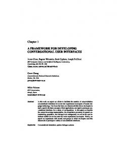
List of Figures Figure 1. Apple Siri answering a weather question .......................................................... 20 Figure 2. WolframAlpha answering a cooking question .................................................. 20 Figure 3. Information retrieval-based QA system procedure [115]. ................................. 21 Figure 4. Hierarchy of ontologies and knowledge base.................................................... 28 Figure 5. Cities within a 10-mile buffer centered at Columbus........................................ 36 Figure 6. Google search for "local open restaurants" ....................................................... 37 Figure 7. Local search on eBay......................................................................................... 38 Figure 8. eBusiness model with geographic local search function ................................... 39 Figure 9. Local search on Facebook ................................................................................. 40 Figure 10. Local search on Twitter ................................................................................... 40 Figure 11. Interaction among components in the framework ........................................... 42 Figure 12. Named entity recognition results of question A .............................................. 45 Figure 13. POS tagging result of question A .................................................................... 47 Figure 14. Basic dependency relationship of question A ................................................. 48 Figure 15. Collapsed dependency relationship of question A .......................................... 49 Figure 16. Context free grammar for question A .............................................................. 50 Figure 17. Probabilistic CFG for question A .................................................................... 52 Figure 18. Parse tree of the part of question A ................................................................. 54 xiii
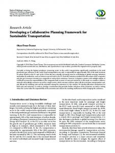
Figure 19. Time complexity of LCS algorithm ................................................................ 56 Figure 20. LCS using dynamic programming................................................................... 58 Figure 21. LCS pseudo code ............................................................................................. 58 Figure 22. LCTS matching ............................................................................................... 59 Figure 23. OGC GeoSPARQL.......................................................................................... 66 Figure 24. DBpedia ontology............................................................................................ 68 Figure 25. Ontology of spatial relationships ..................................................................... 76 Figure 26. Daily Geography Practice................................................................................ 82 Figure 27. Map for raising questions ................................................................................ 85 Figure 28. Procedure of lexical analysis in DGP corpus .................................................. 89 Figure 29. DGP corpus question type distribution............................................................ 91 Figure 30. DGP corpus topic distribution ......................................................................... 92 Figure 31. DGP corpus associated noun distribution........................................................ 93 Figure 32. DGP corpus spatial verb distribution .............................................................. 94 Figure 33. DGP corpus spatial preposition distribution ................................................... 96 Figure 34. Visualization of information gain by splitting on each feature ..................... 100 Figure 35. Class distribution in survey corpus................................................................ 104 Figure 36. Undersample majority class .......................................................................... 104 Figure 37. Oversample minority class ............................................................................ 104 Figure 38. QA user interface waiting for user’s input .................................................... 107 Figure 39. Type A single question output ....................................................................... 108 Figure 40. Type B single question output ....................................................................... 108 xiv
Figure 41. Type C single question output ....................................................................... 108 Figure 42. Type D single question output ....................................................................... 108 Figure 43. Number of templates by number of questions............................................... 110 Figure 44. A reference sentence and tag sequence template. ......................................... 110 Figure 45. A new similar question and its tag sequence. ................................................ 111 Figure 46. Chunk parser.................................................................................................. 112 Figure 47. Ontological reasoning pipeline ...................................................................... 115 Figure 48. GIS labels ...................................................................................................... 116 Figure 49. Type A SQL template .................................................................................... 117 Figure 50. Type B SQL template .................................................................................... 118 Figure 51. Type C SQL template .................................................................................... 118 Figure 52. Type D question spatial SQL template.......................................................... 118 Figure 53. SQL for Type A question “What is the location of Columbus?” .................. 119 Figure 54. SQL for Type A question “Where are Columbus and Cleveland?” .............. 119 Figure 55. SQL for Type B question “the distance between Columbus and Cleveland?” ......................................................................................................................................... 120 Figure 56. SQL for Type C question “the nearest city to Columbus?” .......................... 120 Figure 57. SQL for Type D question “5 nearest cities within 20 miles from Columbus?” ......................................................................................................................................... 120 Figure 58. PostGIS shortest line between two geometries algorithm ............................. 140
xv
Chapter 1: Introduction This chapter reviews the study of question answering (QA) systems in the literature and discusses the rationale of our proposed research. We summarize the advantages of using QA systems for both general and geographic problem solving. We also point out major problems that exist in today’s QA systems for answering geographic questions that involve spatial relationships. Based on a review of several existing QA systems we define the scope of this research and provide an overview of this dissertation.
1.1 Question answering (QA) 1.1.1 Advantages of QA systems Question answering (QA) systems can be useful in both domain specific and open domain applications. A domain refers to a specific field of study such as geography, natural resources, environmental science or public health. Each domain may be further developed into several sub-domains. For example, the geographic domain may include subdomains such as physical geography, human geography and GIS. A domain specific QA system only targets questions within the defined domain, while an open domain QA system is designed to answer questions from all domains.
1
A QA system is beneficial to both non-technical and technical people. QA systems solve problems by providing direct answers to natural language questions. They are beneficial to nontechnical people who may have some level of obstacles for using programs [1] because it’s not necessary to go through each step of analysis to solve problems. Additionally, a QA system may also be used by advanced users to assist their decision making process [2]. A QA system may provide advanced users with immediate access to synthesized knowledge, knowledge summarized from different experts [3], and aggregated information, information accumulated based on historical data [4], for decision making.
Besides the benefits of low technology threshold and quick access to aggregated information, QA system is also known for its dramatically improved efficiency compared with manual approaches of problem solving. Traditional problem solving requires step by step analysis carried out by humans while a QA system can automatically collect information and synthesize them into answers [5, 6]. These answers are often in the form of an exact direct answer rather than a collection of related documents such as provided by a search engine [1, 7].
Another reason for using a QA system is its cross-language characteristics. Much evidence has been found in the literature about using answers in one language to solve questions in another language. Recent studies of cross-language QA systems include
2
systems implemented for solving problems in Chinese [8, 9], Hindi [10], Portuguese[11, 12], Arabic [13, 14], Japanese [15-18] and French [19] among many others.
1.1.2 Open-domain QA systems Open-domain QA systems are designed to answer general questions without a specific topic [20, 21]. Often, an open-domain QA system requires the building of an enormous knowledge base (KB) so that it can answer as many questions as possible. As a result, these systems often make use of various online resources, including web pages, Wikipedia, news articles and blog posts, from which answers are extracted. Open-domain QA systems in the literature include WolframAlpha [22], MIT START [23], MIT DSpace [24], Google Knowledge Graph [25] and IBM Watson [26]. However, none of these systems are sufficient to give a complete answer, if not all, more complicated geographic questions.
1.1.3 Closed-domain QA systems Closed-domain QA systems aim to answer certain type of questions under a specific category [27] such as geographic questions. Although closed-domain QA systems target much fewer types of questions, they are designed to tackle questions that are more indepth and therefore more difficult to answer. This often requires an analysis of the semantics of a question [27] and an incorporation of domain specific knowledge into question answering [28].
3
Recent development of closed domain systems include the following examples: automatic FAQ QA system [29], medical diagnosis QA systems [30, 31], E-Learning QA systems [32, 33], mail auto replay QA system [34], high school algebra word problem QA system [35], project management QA system[36] and e-commerce QA system[37]. All these applications require use of closed-domain systems to service various application needs.
1.1.3 Challenges of QA systems One major challenge to the development of a QA system is its knowledge intensive nature [38, 39]. A QA system requires enormous amounts of general knowledge [40] and domain specific knowledge [6] to understand and answer a question. Such knowledge is often collected from online resources such as Wikipedia, which is often time consuming. On the other hand, as knowledge is often not directly encoded but must be derived from large volumes of data, a QA process is also known for its data intensiveness [41].
To resolve knowledge intensiveness and data intensiveness problems, a QA system must adopt a knowledge-based approach. An information retrieval-based QA system relies on facts extracted from documents for answering questions. By comparison, a knowledgebased QA system relies on both knowledge and facts. Such knowledge includes meta information about facts and inference rules for reasoning with facts. A knowledge-based QA system focuses on resolving the semantics of text in a sentence [42] by using knowledge to analyze semantic structures [43] and semantic roles [44] of different text
4
segments. Many knowledge-driven QA systems rely heavily on ontologies, a computerbased knowledge representation widely used for knowledge intensive tasks [45, 46].
Question answering requires decision making at various steps of processing a question. Decisions are made about sentence separation, question classification, information retrieval and so on. To make decisions, a machine learning (ML) component is often needed, which uses annotated historical data (training data) to predicate the annotation of a new datum [47]. For example, in the case of question classification, an ML-based classifier may be used to classify questions into predefined categories given distributions of historical sentences in each category [48].
ML-based classification may suffer from issues of low efficiency and low accuracy [49, 50]. Among commonly used classifiers, support vector machine (SVM) has proven to be relatively more effective than others on certain datasets [48, 51, 52]; but the problem is it is relatively hard to tune the parameters of a SVM. It is also shown that semantic information in the sentence [53, 54] and question transformation (or paraphrasing) [5557] may be used to further improve ML-based classification accuracy. But these suggestions have yet to be tested in geographic question answering systems.
1.2 Geographic question answering (GeoQA) Geographic questions are common in everyday life. National Geographic Bee (or GeoBee for short) Quiz Challenge features a wealth of geographic questions that may be asked by ordinary people on a daily basis [58]. Question answering games like GeoBee are good 5
ways for 21st century kids to learn geographic knowledge as it guides learning through playing games [59]. Also, quiz books, such as Gaily Geography Practice (GGP), represent other types of resources for learning geographic knowledge through question answering. Although answers to questions in these two applications have already been included, it may be helpful if a GeoQA system can be provided which can answer questions automatically.
1.2.1 Challenges of GeoQA Geographic questions may be challenging to answer in several ways. First, geographic entities in the question are often ambiguous. These entities include place names (e.g. country, state, city, and organization names), street names (e.g. North High Street), zip codes (e.g. 43210), census units (e.g. county, tract and blocks), as well as organization names (e.g. Ohio State University) [60-62]. A city name like Columbus is ambiguous because it could refer to either a city or a person (such as Columbus, OH or Christopher Columbus). Additionally, it may refer to different cities of the same name (Columbus, OH and Columbus, GA). Ambiguity is pervasive in geographic sentences, disambiguation of these entities is an important yet challenging task of a question answering system.
Another type of ambiguity arises from the vagueness inherent in geographic objects. The extent of geographic objects such as cities, mountains and lakes are often vaguely defined because they do not have crisp geographic boundaries [63-65]. For example, we are often 6
not sure where downtown is [66], how big a forest is [65] and what is the extent of Mount Everest [67]. These vague geographic objects are important components of geographic questions but have not been effectively handled in existing systems.
Finally, spatial relationships can also be ambiguous. For example, “near”, “close to”, “around”, and “surrounding” refer to a set of related spatial relationships called proximity. The resolution of these terms provides critical information for distinguishing and interpreting spatial objects involved in the relationship [68]. Spatial relationships may be roughly classified into three categories: directional relations [69-72], topological relations [73-75] and metric relations [76-78]. Both directional and topological relations could be vaguer than metric relationships.
Topological relations infer intersection (or overlay), disjoint, containment relationships between objects. They are often implied by both verbal and prepositional terms such as “touches”, “borders”, “within”, “on” and “in”. Directional relationships are conveyed in azimuthal terms such as “north”, “south”, “west” and “east” or relative directional phrases such as “in front of” and “to the north of”. Metric relation terms involve a quantitative term and a spatial relationship term. For example, “cities within 10 miles from Columbus” is an example of defining metric relationship between Columbus and other cities. Any of these relations may easily appear in any geographic question, but they have not been systematically discussed in the literature in the question answering context.
7
Efforts have been made in the literature on the disambiguation of geographic terms. The goal of disambiguating geographic entities is to ground them onto the earth surface [7981]. Ontologies are knowledge of kinds and relationships between entities [82]. Ontologies may be used to represent both general knowledge and geographic knowledge [83-86] but the use of ontology lacks discussion in a GeoQA context. It is possible and potentially beneficial to integrate geographic information system (GIS) techniques into the implementation of a GeoQA system. GIS provides sophisticated functions for spatial data modeling, manipulation and analysis [87-90] which may not be available in other systems. Spatial data handling capabilities of a GIS may provide problem solving expertise to a question answering system and therefore may potentially help answer more complicated geographic questions; however few efforts have been made in the literature in using GIS for question answering.
1.2.3 Major problems in GeoQA There are open domain systems that can answer geographic questions but few of them can answer in-depth geographic questions. These in-depth geographic questions include spatial entities and relationships that often require geographic knowledge system such as a GIS to resolve. To solve in-depth geographic questions using GIS, one must come up with ways of representing spatial entities using geometries and converting spatial relationships into GIS operations. However, there is a great lack of research in the literature in this regard.
8
Most of QA systems that can answer geographic questions are implemented by computer scientists instead of geographers. This causes some problems to the design of the system partly because computer scientists may not intentionally use knowledge outside their domain, such as spatial knowledge and the use of GIS in this case, to implement an open domain QA system. Spatial knowledge like spatial thinking (or spatial cognition) [91-94], spatial abstraction [95-98], spatial association [99-102] and spatial generalization [103106] are essential to solve most non-trivial geographic problems. However, these spatial skills are largely neglected by computer scientists for designing a QA system for answering geographic questions.
Current QA systems for answering geographic questions suffer from the lack of spatial inference rules. These rules are used to determine the spatial relationship between objects or identify objects based on their spatial relationships. These rules involves definitions of spatial objects and relations between these objects [107, 108]. Spatial inference rules implement mental spatial reasoning of humans and can be differentiated into qualitative and quantitative spatial reasoning [70, 72, 109, 110]. Quantitative spatial reasoning, such as proximity reasoning, often involves the generation of an extended area from a spatial object, favourably called a buffer area. Such a buffer area may not pre-exist in any form of available knowledge but must be derived from knowledge primitives using spatial functions in a GIS.
9
Current QA systems assume facts are static while geographic facts could be changing over time. Specifically, geographic objects may change its location and extent under various spatial temporal circumstances [111-114]; consequently, an object in the database may not always be grounded to the same location at different times of queries. For example, political and census boundaries are indeterministic due to changes in census statistics. Same are congressional districts and voting districts. Living objects like humans, animals, or automobiles also tend to relocate over space by time. As a result, a question answering system involving such objects must consistently update its knowledge base based on the latest location information of objects.
1.3 Previous approaches to geographic QA In this section, we review a few classic QA systems and compare their question answering architectures. Our goal is to generalize essential components from their various frameworks to implement our own geographic question answering system.
1.3.1 Annotation-based approach Annotation-based approach is relying on facts for answering questions. Facts are stored in triple stores. They are the knowledge databases which include individual records as a triple. The MIT START system is capable of answering several types of geographic questions based on triple stores. The START system first annotates facts in documents. Then, it transforms all annotated facts into ternary
10
expressions (T-expression), [23]. The following is an example [23]: The sentence “Bill surprised Hillary with his answer” will produce two T-expressions:
Based on T-expression formation of knowledge, their QA system is built in four steps: (1) Collect raw data from Wikipedia in terms of text and images. (2) Annotate each piece of data in the form of ternary expressions. (3) Generate START knowledge base using T-expressions. (4) Answer questions by searching and relating facts in the knowledge base.
Although START can answer many questions involving general geographic knowledge; it cannot yet answer many other geographic questions whose answers are not encoded in Wikipedia or anywhere else on the Web. For example, asking the question “what cities are within 100 miles of Columbus” to the system returns nothing. This may be because START system is not designed to answer this type of question; or it may have certain deficiencies for dealing with this type of geographic questions: (1) Facts for answers must be available in the knowledge base. There is no mechanism to generate new facts. (2) Lack expert knowledge and spatial intelligence for processing geographic information including information about spatial entities and spatial relationships.
11
1.3.2 IBM Watson: the deep QA approach The most famous QA system in practice may be the IBM’s Watson system. In the Jeopardy challenge game, Watson beat the best human contestant on various categories of questions. From a research paper by its developers, we find Watson’s superior QA capabilities are primarily supported by four components (Ferrucci et al. 2010): (1) Massive parallelism: A question can be interpreted in different ways. The Watson team exploited massive parallelism in the consideration of multiple hypotheses of interpreting a question. (2) Many experts: Watson facilitates the integration, application, and context-based evaluation of a wide range of loosely coupled probabilistic reasoning. (3) Pervasive confidence estimation: All components score features for question answering and no single component commits to an answer. (4) Integration of both shallow and deep knowledge: Watson balances the use of strict semantics and shallow semantics, leveraging many loosely formed ontologies to improve inference efficiency.
Even with these sophisticated implementations, Watson still didn’t manage to answer one question correctly “The category was U.S. Cities, and the answer was: ‘Its largest airport was named for a World War II hero; its second largest, for a World War II battle.’ The two human contestants wrote “What is Chicago?” for its two airports O’Hare and Midway, but Watson’s response was “What is Toronto?”
12
According the David Ferrucci, the manager of the Watson project at IBM, Watson was confused on this question for several possible reasons. First, the answer doesn’t exactly fit the category. Second, Toronto in Canada is related to U.S. through American League baseball team. Third, there are cities named Toronto in the United States although none of these cities have airports. It seems that Watson made mistakes by relating Toronto and U.S. through a series of weak inferences.
1.4 Purpose of This Study The purpose of this study is to design and implement a closed-domain GeoQA system that can answer some types of geographic questions for which traditional QA systems are not designed or may not be able to answer. To do this, we developed ontologies of space to interpret the meanings of spatial terms in natural language questions. Ontologies are categories of various types of knowledge and the relationships between them. Previously, ontologies of space have been studied mainly from the conceptual perspective but have yet to be incorporated into real world applications. There is also a shortage in the research of ontologies of spatial relationships.
Additionally, this study incorporated geographic information system (GIS) techniques to solve the problems associated with the answering of geographic questions. There is great potential for employing spatial data modeling and analysis of GIS for the implementation of QA systems that are capable of answering more in-depth geographic questions. However, there is a dearth of research in this area. Unlike previous research, our systems do not extract answers by structure matching but instead rely on geometric 13
representations of spatial entities, semantic interpretations of spatial relationships and mapping of entities and relationships to GIS data and operations. Finally, the problem of question answering is converted to query a spatial database via executing a spatial SQL.
By utilizing spatial functions provided by a GIS, our proposed GeoQA system does not require an enormous amount of data to be able to answer a large number of questions. In fact, our system is designed to be able to answer a theoretically unlimited number of questions mainly based on knowledge primitives, basic elements of information, and a GIS. These elements are atomic components of spatial objects, such as their identities, locations and other essential attributes. GIS serves as the data engine to provide inference capabilities between these spatial objects.
To implement our proposed system, first this study investigated the nature of geographic question formation by analyzing two corpus of geographic questions. Daily Geographic Practice were analyzed to determine the components involved in a geographic question. These components included question types, topics and use of words, and so on. Based on observations from corpus analysis, our goal was to develop an ad hoc survey of all the necessary components, which comprise the experimental purpose of this research.
We further proposed a synergistic framework involving several interacting components to answer geographic questions. Several essential components are required by this framework, including natural language processing, machine learning, ontological 14
modeling and geographic information systems. The natural language processing (NLP) component examines syntactic and lexical patterns of a sentence while separating out useful information for subsequent analysis. We implemented part of speech taggers to syntactically analyze sentences and a chunk parser to extract geographic information from a sentence. A machine learning component was mainly used as a classifier to sort sentences. We implemented a machine learning component to train a classifier using annotated examples and to classify new sentences based on the dynamic programming longest common sequence matching algorithm and voting algorithm.
We also developed ontologies of space to interpret meanings of a sentence. Ontologies of space were developed to disambiguate spatial entities and model them in a GIS. These include ontologies of concrete space, abstract and linked space. Ontologies of concrete space are necessary for determining various types of spatial entities. Ontologies of abstract space are needed to represent spatial entities as geometries which are necessary for GIS processing. Ontologies of linked space may be used to map entity types to possible geometric representations in a GIS. Ontologies of spatial relationships need also be developed, which are necessary for determining the type of operations required for solving geographic questions. Lastly, the geographic information system component was programmed to construct formal queries using information extracted from sentences. Results will be turned from spatial databases via spatial SQL queries.
15
Finally, our demonstration system was able to answer four categories of geographic questions: location, distance, proximity entity and proximity buffer questions. Due to the complexity of implementing a real world question answering system, the purpose of this study was not to answer all types of possible geographic questions but to demonstrate the adaptability of our framework for answering more geographic questions using GIS. More importantly, we hope our study of ontologies of space and spatial relationships as well as the use of GIS for answering questions may shed some light on further natural language research in both geography and computer science fields.
1.5 An Overview of This Thesis The remainder of the paper is organized as follows. Chapter 2 is a review of the underpinning techniques for programming traditional QA systems. Four types of related techniques are discussed for answering geographic questions: natural language processing, machine learning, ontologies and GIS. Chapter 3 discusses our proposed geographic question answering framework and four essential components that are included in this framework. Chapter 4 introduces the data for experiments in this research including spatial data, attribute data and corpus data. Chapter 5 includes the analysis results of two types of corpus: daily geography practice corpus and survey corpus. Chapter 6 covers the implementation, results and evaluation of the system. Chapter 7 discusses how to extend the current application to answer more questions. Chapter 8 contains the conclusion and suggestions for future studies.
16
Chapter 2 Underpinning Technologies
2.1 Natural language processing Natural language processing (NLP) is a fundamental component to question answering (QA). It is concerned with both syntactic and semantic analysis of a sentence based on key techniques like tokenization, part of speech (POS) tagging and parsing [115]. A syntactic analysis boils down a sentence to a sequence of POS tags which conveys the function of a word. For example, the POS tag of the word Columbus is nominal proper noun (NNP); this word can follow a preposition (PP) like in. A semantic analysis resolves the meaning of each tag. Both syntactic and semantic analyses are two interacting aspects of understanding a sentence. NLP is related to various steps of building a traditional QA systems such as document retrieval, information retrieval and feature extraction. Here, we review the use of NLP in building some state of the art NLP-based QA systems.
2.1.1 Structure matching One of those first QA systems is based on the “structure matching techniques” [116]. Such systems look for answers to a question by examining structured information about entities and their relationships in a sentence. There is no agreed definition of structured information; but it may be generally defined as information stored with properties and relationships. Examples of structured information are tables, relational databases and 17
xmls. These structured information can be retrieved more easily than non-structured information (such as raw web pages) for constructing answers for a question. The following example is given [117] For example, to answer the question “What do birds eat?” the system first extracts the structure of question as [birds] → [eat] → [what] , in more generalized form [what]→[eat]→[worm]. Table 1 lists a few candidate sentences that might be scanned along with some structures extracted from each sentence. By matching the structure of the question with those in the table, the system may find that worm is the answer.
Sentence Worms eat grass. Horses with worms eat grass. Birds eat worm. Grass is eaten by worms.
Structures [Worms]→[eat]→[grass] [Horses] → [with] → [worms] [Horses] → [eat] → [grass] [Birds] → [eat] → [worm] [worms] → [eat] → [Grass] Table 1. Sentence and structures
Many contemporary systems are backboned by an NLP engine using variations of structure matching technique like the one above. IBM’s Watson can beat the best human Jeopardy contestant on questions like “In 1903, with presidential permission, Morris Michtom began marketing these toys.” and the answer is “What are teddy bears?” Other systems can provide interactive dialogs. For example, in Fig. 1 Apple’s Siri can answer questions like “What’s the whether like tomorrow in Columbus, OH?” and an answer including temperature information will be provided. One may further add additional questions like “how about the day after tomorrow?”. Siri can also provide answers based 18
on all information to date. In Fig. 2 WolframAlpha push the question answering frontier even further by providing answers with rich contents. The figure below is an example of answering the question “time to cook a 20 lb turkey?” on WolframAlpha.
19
Figure 1. Apple Siri answering a weather question
Figure 2. WolframAlpha answering a cooking question
20
2.1.2 NLP for information retrieval One important use of NLP for QA is to retrieve information from sentences. Information retrieval extracts phrases from documents and reorganizes them as answers [118, 119]. As in Fig. 3, an information retrieval-based QA system mainly follows three steps of analyzing a sentence: question processing, passage retrieval, and answer processing. In question processing, sentences are analyzed and formed into queries. It also includes a step of classification of questions into predefined categories such as location question, person question, and so on. These categories are important because they provide necessary information for constructing answers using correct information. For example, a person question expects a person name rather than a place name as an answer although both names may both be nouns and look similar in forms. Later, relevant passages in all documents are retrieved and answers are constructed based on retrieved information during answer processing. NLP is used in all three steps; but here we only discuss the first step, question processing, because it is this step is common across different approaches.
Figure 3. Information retrieval-based QA system procedure [115]. 21
The goal of question processing is to generate two inputs to a QA system: first, a keyword query suitable as input to an information retrieval system; and second, an answer type, a specification of the kind of entity that would constitute a reasonable answer to the question [115].
2.1.2.1 Query processing How queries should be formed depends on each application. For example, in the case of using a search engine for finding answers, we might simply create a keyword list including all the words in the question as the search engine would automatically remove the stop words--words which are often skipped during the processing of natural language text such as a, an and the. Alternatively in other cases, only noun phrases may provide useful information and therefore the keyword lists should only include the noun phrases.
To what extent a keyword query can be useful to retrieve answers is subject to the variations of a query and the size of the document base. Queries may vary in forms and use of lexicons. A sentence of the same meaning may be expressed in many different ways. However, based on fewer documents of retrieving information an exact match of a document including the answer is unlikely to happen. Therefore we need to apply a technique called query expansion that can be used to transform existing terms in the sentence to additional related forms hoping to match a particular form of the answer in the document base [115]. Table 2 lists two commonly used query expansion methods: morphological expansion expands a query by replacing a word with its stems and lemmas 22
and rule-based rephrasing expands a query by changing the order of elements in the sentence based on transformation rules [115].
Query Expansion Method
Techniques
morphological expansion
Stemming Lemmatization rephrasing
Resources That Can be Used
WordNet, domain specific thesaurus rule-based rephrasing Question to declaration transformation Table 2. Query expansion methods.
Stemming refers to a crude heuristic process that chops off the ends of words. It is hoped that the remaining segment can keep most part of the meaning of the original word. Lemmatization refers to morphological analysis of words, normally aiming to remove inflectional endings only and return the base or dictionary form of a word, which is known as the lemma [115]. For example, the word having has its stem hav and lemma have. However, stemmers are typically easier to implement and run faster, and the reduced accuracy may not matter for some applications.
The rule-based rephrasing aims to make a question look like a declarative sentence. For example the question “where is Columbus located?” would be rephrased as “Columbus is located”. Rule-based rephrasing changes a sentence by reordering its lexicals but does not alter its meaning of a sentence.
2.1.2.2 Question classification
23
Question processing always includes the step of classifying a sentence into answerable categories. This is to make sure that a QA system knows what type of answers are expected [115]. The number of the classification varies with applications [48, 120]. A classification is more granulated if it has more classes for questions to fall into. In most cases, the starting few words of a question should include enough information for classification. For example, a question like “Who founded Apple?” warrants an answer of type PERSON. In this case, a rule-based type detection method can be developed. Another question such as “What Chinese city has the largest population?” expects an answer of type CITY as indicated by question word what and head noun (first noun) city. But the noun does not have to be city here; for example town may convey the equally same meaning here according to ontologies of concrete space which will be discussed later.
In this research, we need a method for classifying geographic questions. Geographic questions often include spatial entities and spatial relationships. This information is critical for determining how a question should be answered using a GIS. In this research, we plan to propose a new classification scheme which classifies questions based on GIS operations needed to solve them. GIS operations include distance, buffer, spatial relationship operations and object measurement. Studies of these operations in a question answering context are few in the literature.
2.1.2.3 Focus detection 24
After classification, a classic information retrieval-based QA system will detect what is the focus of the sentence and extract relations between entities. Focus is the main subject mentioned in a sentence. Focus detection refers to finding what in a question should be replaced by an answer. Relation extraction refers to finding relations between entities in the question. Relations between entities constitute one of the most important aspect of knowledge that can be used to infer answers. A triple is an effective format to model such a relation: relation (A,B) For example, Capitol (“Columbus”,”Ohio”), Border(“Ohio”,”Kentucky”) are such relations. These relations may be either manually established or drawn from online knowledge repository such as Wikipedia, infoboxes, DBpedia, FreeBase, and so on.
Here is an example of detecting the focus and extracting relations from a question. Question: What are the two states you could enter if you cross Ohio’s southern border? Answer type: (U.S.) states. Query keywords: two states, Ohio, south border. Focus: two states (because this is what should be replaced by an answer) Relations: border (south of Ohio, ?x). ?x means any match of entities. In documents that include answers, we are looking for declarative statements such as “Kentucky borders south of Ohio,” “Ohio borders Kentucky in its south” and “The southern border of Ohio touches Kentucky.” 25
2.2 Machine learning Machine learning is concerned with a program and/or a system that is capable to learn and improve their performance on a certain task over time [121]. Machine learning (ML) is used at various decision making steps of question answering process such as question classification, passage rank, answer extraction and evaluation. In all these tasks, ML is mainly used to develop a classifier, a program to classify data, through training classified data set. For example, in the process of part of speech (POS) tagging, a POS tag classifier is trained based on annotations of tags for each sentence. Later, this classifier is used to assign POS tags to words in new sentences.
Relating to QA, a common usage of machine learning technique is to classify questions. There are several different ways of classifying a question. One way is to classify a question based on its subject type. For example, if the question is asking about a city, it will be a city question. This is most commonly used method in the literature. Another way is to classify the question based on the type of processing procedures needed to answer the question, that is, the number and type of steps needed to answer a type of question. This method is not discussed in the literature but will be used in this research.
One of the common machine learning techniques is supervised learning. Supervised learning is often used in QA system. Supervised learning refers to a set of techniques that 26
generate a function to map inputs to a desired class label, a class label that correctly annotate the input [122]. Particularly, the label could have either a binary value or multiple values. In the context of question answering, for example, a binary value label may be used to tag a question as either [geographic] or [non-geographic]. By comparison, a multivalued label can be further used to classify what types of geographic questions are asked more specifically: [location], [city], [buffer], and so on. The most commonly used supervised learning algorithms include logistic regression, naïve bayes, decision trees, and support vector machines (SVMs).
In contrast, unsupervised learning refers to a set of techniques that try to find clusters from a set of unlabelled inputs without manual human annotations. Therefore, unsupervised learning is also called clustering [123]. ML clustering algorithms are used to find natural groupings and patterns from the data. In practice, clusters of data are found based on some similarity measures. Common cluster algorithms include K-means, hierarchical clustering, principle component analysis (PCA) among others. Finally, semisupervised learning refers to any technique that generates a mapping function with both labelled data and unlabeled data; a combination of both supervised and unsupervised learning [123].
27
2.3 Ontology 2.3.1 Ontology and knowledge base Computationally, ontologies are explicit specifications of shared conceptualization for computer programs [124]. Shared conceptualization requires that concepts of entities and relations in the ontology must be commonly acceptable by ordinary people or people Figure 4. Hierarchy of ontologies and knowledge base from a domain. Explicit specification refers to a set of rules for defining and accessing ontologies [82].
An ontology is a type of higher level of knowledge, or meta-knowledge. Such metaknowledge defines the vocabulary, axioms and hierarchy that can be used to describe lower level knowledge such as facts of reality or instances of conceptualization [125]. By comparison, traditional knowledge base consists of only low level facts about the reality. Such knowledge are normally encoded in unstructured documents, structured relational databases or triple bases. Fig. 4 shows the relationship between ontologies and knowledge base.
28
Mediator Ontology Schema
Schema
Schema
KB
KB
KB
2.3.2 Types of human knowledge To develop ontologies, it is important to come up with a taxonomy of human knowledge first. Here, we include a list of common types of human knowledge and discuss the characteristics of each type of knowledge in Table 3 (adapted from [126] and [127]) Category *Procedural knowledge *Declarative knowledge
Subtype Rules, strategies, agendas, procedures Concepts, objects, facts
Metaknowledge
Knowledge about how to use knowledge Rules of thumb
*Heuristic knowledge *Structural knowledge Inexact and uncertain knowledge Common sense knowledge
Rule sets, concept relationships, concept-to-object relationships Probabilities, uncertain facts, rules, relationships, and evidence, fuzzy sets and logic Default propositions, approximate concepts and theories, general hierarchies and analogies 29
Geospatial Implications Geoprocessing steps for solving a geographic problem. Geographic entity types and spatial relationship types. Instances of geographic entities. Facts about entities and relationships. Knowledge about how to use geographic knowledge. Experience from GIS expert for solving similar problems. Is-part-of, is-whole-of, is-sumof, is-grouping-of relationships between different geographic entities. Ambiguous spatial terms. Qualitative spatial constraints. Common sense geographic knowledge, such as knowledge about the world.
Table 3. Types of human knowledge1.
2.3.4 Ontological representation of knowledge There are two components that must be included in the definition of a computational ontology: vocabulary and taxonomy [127]. A vocabulary is a set of natural language terms for describing different types of entities in the domain. Vocabulary in ontology must be unique and unambiguous, which is different from that in real life such as English vocabulary in a dictionary. The vocabulary of geographic ontologies should define a set of unambiguous terms pointing to different types of entities. For example, in real life the terms city and metropolis may mean different things to different people; but in ontological vocabulary, city and metropolis may be defined as equivalent types or as members of a unique type city. Different from a vocabulary which is concerned with concepts, a taxonomy defines a hierarchy of concepts. These relationships are often defined as super-class relationship or sub-class relationship between different types or amember-of relationship between a type and its instances. For example, ‘administrative unit’ could be defined as a super-class of the concept city and Columbus could be defined as a member of the concept city.
1
indicates the type of knowledge are most needed for geographic question answering.
30
2.3.5 Spatial ontologies Ontologies are used to attack knowledge intensive problems [128, 129]. Geographic question answering is knowledge intensive in that it requires not only knowledge of spatial entities but also knowledge of entities relations [85, 130]. Spatial reasoning is concerned with both representation of spatial entities as different types of geometries and inference of spatial objects based on spatial relationships.
Spatial entities can be concrete objects like cities, places as well as abstract entities like points, lines and polygons. Spatial relationships include topological relations such as (dis)joint, overlap and intersect as well as metric relations such as the percentage of overlap. Modeling spatial ontologies requires formalization of both spatial entity class and spatial relationship class as well as rules for reasoning between instances of these classes. We will discuss more details of spatial ontologies later.
2.4 Geographic information systems Geographic information systems (GIS) may be defined as a computer-based system that enables capture, modeling, manipulation, retrieval, analysis and presentation of geographically referenced data [131]. GIS are a popular tool for data analysis because a lot of information contains a spatial component.
The core of GIS is a set of spatial analytical tools that can be used to store and process spatial data. Typical tools include those that can be used to create spatial objects, resolve spatial relationships, and derive new objects based on certain spatial process. More 31
advanced tools can be used to build a model or to run a simulation. However, most advanced tools in GIS are ad hoc in nature and can’t be easily replicated to other GIS.
Commercial GIS such as ESRI’s ArcGIS may provide a more comprehensive suite of tools for processing, analysing and modeling geographic data. Due to cost and availability reasons, open source GIS such as Quantum GIS (GIS), uDig and GRASS GIS are also popular. Notably, GIS doesn’t have to be a desktop software with interfaces; spatial database can also serve as a GIS too. In this research, we use spatial database PostGIS as the GIS backend for solving geographic questions.
Spatial databases are often extended from underlying relational databases. Table 4 lists some popular relational databases and their corresponding spatial extensions.
Relational Database Sqlite IBM DB2 Oracle Microsoft SQL Server PostgreSQL MySQL
Spatial Extension SpatiaLite IBM DB2 Spatial Extender Oracle Spatial Internally support spatial types since version 2008 PostGIS Internally support more spatial functions since version 5.6 Table 4. Spatial databases
The spatial functions provided by GIS may be very useful for answering more complicated natural language questions. These questions normally involve spatial relationships and requires spatial operators to process geographic information in the question. However, there is a great lack of research in this regard in the literature. In this 32
research, we attempt to bridge natural language analysis of geographic sentences to GIS processing via the use of ontologies of space. We will talk about ontologies of space in next chapter.
33
Chapter 3 Framework and System Components One of the objectives of this research is to develop a framework for processing geographic question with spatial entities and relationships involved. Also, this research attempts to solve GeoQA problems without harvesting the knowledge on the web but to the greatest extent relies on spatial knowledge for solving problems. Such knowledge is encoded in terms of facts in a spatial relational database as well as knowledge of processing spatial data provided by a GIS. This chapter first discuss why knowledge of GIS is important for building a GeoQA system. Then it gives an example of the type of geographic question that is targeted in this research and discusses potential applications that may benefit from findings of this research. Finally, a framework is proposed to solve the type of questions we target on in this research.
3.1 GIS as The Foundation of Knowledge-based QA Systems IR-based QA systems rely on information in documents to search for answers; however, many geographic questions are difficult to answer using IR-based QA systems. This is largely because spatial information, such as spatial relationships between objects, are often not coded in regular documents but stored as procedural knowledge in our mind. Such knowledge, however, is widely available in most GIS systems and is easily accessible through database functions or application programming interfaces.
34
GIS may be used as a backend processing tool for solving geographic questions. In-depth questions are those that require resolution of spatial entities, spatial relational aspects and spatial operations for answering questions. GIS has a suite of spatial reasoning functions that could be used for these purposes, so, we proposed a GIS-based framework for this purpose.
3.2 An Example of a Geographic Question Used in This Research A GIS-based QA system uses knowledge primitives and spatial inference rules to answer questions. Knowledge primitives are the smallest units of knowledge about reality that are necessary to identify, characterize and discriminate between entities. Examples of geographic knowledge primitives are names of geographic entities as well as their locations and classes. Below is an example of the type of questions that may be answered by a GIS, by not by a traditional QA systems: What are the five nearest major cities within 10 miles from Columbus?
The answers are the following cities: Grandview Heights
2.7 miles away
Bexley
3.54 miles away
Upper Arlington
4.48 miles away
Whitehall
6.01 miles away
Gahanna
6.97 miles away
35
Figure 5. Cities within a 10-mile buffer centered at Columbus
3.3 Potential applications Although one may argue that the above example may not be a typical one that people ask on a daily basis, a GeoQA system that can solve similar questions shed light on many potential applications such as intelligent search, social networking and e-business. Here we give a few more examples one may think of which may make use of our proposed GeoQA system.
3.3.1 Internet search Google, Bing and Yahoo: Current Google search is not quite able to answer questions like “what restaurants within 5 miles from me are currently open?” This suggests the type of information one may 36
want to know on a daily basis. However, currently Google could only return no more than a list of related web pages about restaurants but no direct, or even close, answers are given. One may also argue Google is not designed for this type of search but we only argue here that to be able to answer this type of question in Google may benefit Internet users.
Figure 6. Google search for "local open restaurants"
3.2.2 Local business search via Amazon, eBay, Craigslist, PayPal Currently, business models on Amazon and eBay are based on transactions through shipping via postal mails. An item is purchased and shipped to a buyer regardless of the relative location between the buyer and the product. However, opportunities exist for local sellers and buyers to do business offline. For example, a buyer could search 37
products locally and find nearby sellers. This e-business model has several potential advantages. First, buyer could see real products before buying it. Second, sellers may save shipping cost of the goods. Third, transactions of large and heavy items are more possible via local pickup than through shipping. Finally, local transactions popularize the exchange of many used items.
Although eBay allows items to be locally picked up by a buyer from a seller, currently, there is no way for users to search items locally. For example, asking the following question on eBay will return nothing “find me used road bikes within 10 miles from 43210”.
Figure 7. Local search on eBay
Craigslist, a classified advertisement website, may also benefit from our proposed GeoQA system. However, no functions on their site supports searching items on a 38
geographic basis using natural language query. Here is a model we develop to illustrate how vendors may benefit their e-business activities by incorporating a geographic natural language search component.
Figure 8. eBusiness model with geographic local search function
3.2.3 Local search on social network sites such as Facebook and Twitter Currently, neither Facebook nor Twitter supports geographic natural language search. For example, searching “status updates within 10 miles from me” redirects Facebook to Bing. Searching “hot tweets 10 miles from me” on Twitter returns nothing. However, such search functions may be potentially useful for users to explore various interesting topics on their sites.
39
Figure 9. Local search on Facebook
Figure 10. Local search on Twitter
3.4 The GeoQA Framework and System Components Our proposed framework consists of four components: natural language processing (NLP), machine learning (ML), ontology reasoning (OR) and a geographic information 40
system (GIS). Table 5 lists these components as well as typical tasks of each. Also, we discuss the role of each component in answering geographic questions.
Components NLP component
ML component Ontology component GIS component
Tasks Parse sentence into semantic components. Extract features from sentence for classification.
Techniques Tokenization. Part of speech tagging. Lemmatization. Parsing. Named entity recognition. Train classifiers using training Annotation. corpus sets. Supervised learning Classify new question. classification. Discriminating the semantics of Ontological modeling and spatial terms. reasoning. Abstract linguistic entities into Spatial data manipulation spatial representations. functions. Map spatial relationship terms to Spatial relationship functions. GIS operations. Spatial measurement functions. Table 5. The framework
3.4.1 Natural Language Processing Component The NLP component is the most fundamental of all four components. It interacts with the machine learning component by providing features for training classifiers and classification. As previously discussed, most linguistic features are either lexical-based or tag-based. NLP techniques for extracting these features will be discussed in later chapters. The NLP component also interacts with GIS through ontologies. An ontology transforms the mapping from linguistic terms to GIS data and operations. Fig. 11 shows the interactive relationship among the four components. Arrows indicate data flow.
41
Figure 11. Interaction among components in the framework
Next, we discuss various NLP techniques in greater detail for processing geographic questions. These techniques work together in a pipeline to provide a fully functional analysis of natural language. Below is an example of the processing of a typical question, Question A: What are the five nearest cities within 20 miles from Columbus?
3.4.1.1 Tokenization Tokenization is the process of separating out (tokenizing) lexical units from running text. A lexical unit could be either a word or a letter depending upon the application. However, in most cases, word tokenizer is assumed by default because most applications analyze words rather than individual letters. Depending on the requirements of the application, 42
compound words could be considered as a single unit. For example, Ohio State University and post office are both considered as a single word according to common sense knowledge despite the fact that they contain spaces in between. For this purpose, a compound word dictionary may be necessary for establishing a tokenization algorithm. Similarly, a noun phrase tokenizer will not separate words in a noun phrase as individual tokens. In this sense, a tokenizer is similar to a chunker, or named entity recognizer, which will be discussed in later chapters.
Tokenization results for question A are given in Table 6. Tokens are separated by commas. A tokenizer is a program that separates elements of a sentence. A noun phrase tokenizer is a tokenizer that does not separate noun phrases.
Word tokenizer Alphabet tokenizer Noun phrase tokenizer
What,are,the,five,nearest,cities,within,20,miles,from,Columbus,? W,h,a,t,a,r,e,t,h,e,f,i,v,e,n,e,a,r,e,s,t,c,i,t,I,e,s,w,i,t,h,i,n, 2,0,m,i,l,e,s,f,r,o,m,C,o,l,u,m,b,u,s,? What,are,the five nearest cities,within,20 miles,from,Columbus,? Table 6. Tokenization results of question A
3.4.1.2 Sentence Segmentation Sentence segmentation, separating sentences from one another in a paragraph or document, is related to tokenization. In a dialog-based question answering system, a question may be made up of a sequence of sentences in which sentence segmentation will be necessary for understanding what is being asked. Sentence segmentation is generally 43
based on punctuation, including periods, question marks, and exclamation points that normally indicate sentence boundaries. Exclamation points and question marks are relatively unambiguous markers of sentence boundaries. By comparison, periods may not indicate a boundary, as in the case of abbreviations like Ms. or Inc.
3.4.1.3 Named Entity Recognition Named entity recognition (NER) is the process of detecting and classifying named entities. A named entity refers to the number of words in a sentence that can be associated with a proper name, such as names of people, organizations, and places. Named entities can be detected by locating proper nouns in a sentence. In English, these proper nouns are normally words that begin with capital letters.
Classification of named entities requires a dictionary to link entities with their types. Hierarchies can also be defined in the classification. For example, subtypes of named entities can be grouped into super types. Creating a taxonomy of geographic named entities is important for determining their geometric types for data modeling in a GIS. Table 7 is an example of classifying geographic named entities. Our demonstration system contained only the category city, but did not include all types of entities.
44
Named Entity Type Organization
Categories
Geometric Types
companies, universities, polygon, point, multi-polygon, multisports teams points; Physical mountains, lakes, oceans, polygon, polyline, point; multiEntity rivers, ponds polygon, multi-polyline, multi-polygon; Administrative countries, states, provinces, polygon, point, multi-polygon, multiEntity counties, cities points; Political state, congressional district, polygon, point, multi-polygon, multiEntity voting district points; Transportation bridges, bus stop, airports point, polyline, multi-points; Facility Point of restaurants, shops, parks polygon, point, multi-polygon, multiinterest points; Table 7. Geographic named entity classification
The NER result of question A is shown in Fig. 12. This result is generated using brat, an online tool for annotating named entities in a sentence [132]. One may potentially use other tools; however, brat assigns a color to each annotation, which we find effective for the purpose of illustration. As we can see, the default brat tool developer detects two types of named entities: numbers and locations. However, it does not further differentiate the type of location.
Figure 12. Named entity recognition results of question A
In our system, our customized NER produced the following results with entity types annotated in the subscript. The implementation of the system will be discussed in greater detail in the next chapter. What are the five NUM nearest cities within 20 NUM miles from Columbus CITY 45
3.4.1.4 Parts-of-speech tagging Parts-of-speech (POS) tagging is used to assign a part of speech tag or syntactic class to each token of a sentence. A token could be a word, a punctuation or any content separated by two adjacent spaces in general. The single best POS tag assigned to a word depends on both the function of the word in context and the tag set used for the task. The most common tag set is brown and includes 87 tags, while the Penn Treebank tag set includes 36 tags [133]. POS tagging is essential for determining the pronunciation of a word and interpreting its meaning.
Tagging is challenge in NLP analysis because most tokens are ambiguous. This is because a word can have multiple senses each of which may result in a different POS tag. For example, the word “touch” in the phrase “the touch of the waves” is a noun, while “the state Ohio touches” is a verb. Attempts at improving POS tagging have included various algorithms, such as rule-based, probability-based and machine learning algorithms [115]. Rule-based taggers use a set of guidelines provided by linguistics experts to determine which tag should be assigned to which component. For example, the word after a modal should be a verb. An example of taggers are the EngCG or the Brill Tagger. The probability-based approach relies on probability distribution generated from a training corpus. Examples include HMM-based taggers. Machine learning-based algorithms transform tagging tasks into classification problems. Methods such as SVM, maximum entropy, perception, and nearest-neighbor have all been previously studied.
46
Overall, contemporary POS taggers can reach an average accuracy of above 95% on tokens but only a 56% accuracy on sentences [134]. Low accuracy is often caused by differences between the training and test sets on topics and styles, as well as differences in the training size and type of taggers [134]. Efforts have been made to develop tagging algorithms to improve both tagging performance (i.e. speed) and accuracy (i.e. percentage of accuracy) including dynamic programming-based Viterbi, rule-based Brill taggers, maximum entropy taggers and neural network-based taggers. For a complete list of tagger comparisons, one may take a look at the ACL wiki page on POS tagging [135]. The POS tagging result of question A is shown in Fig. 13. The result was found using the Penn Tree bank tags and Stanford POS taggers [136].
Figure 13. POS tagging result of question A
3.4.1.5 Constituents A group of words that function as a single grammatical unit within a sentence is called a constituent. For example, a noun phrase, prepositional, adjective and adverb phrase are all constituents. The concept of constituent is related to sentence parsing in which each node represents a constituent except the root node and leaf nodes. The extraction of constituents in question A will be explained in the parsing section.
3.4.1.6 Grammatical relationships 47
This term refers to the relationship between grammatical components in a sentence. For example, subject and object are two grammatical components. In the following sentence, Ohio borders Kentucky. Ohio is the subject and Kentucky is the object. The following is an analysis of the grammatical relationships within question A: [What] SUBJECT are [the five nearest cities] OBJECT within 20NUM miles from Columbus?
3.4.1.7 Dependency Relationships Dependency relationships show which words depend on which other words in terms of modification and argument relationships. Question A’s basic dependency structure is shown in Fig. 14. The arrow in the graph indicates a modifying or argument of relationship. For example, A → B means A’s modifier is B if B is before A or A’s argument is B if B is after A. In Fig. 14, we can see the five nearest are all modifiers of cities. Within is also a modifier of cities, while miles is a modifier of within.
Figure 14. Basic dependency relationship of question A
Collapsed dependency tends to group certain dependencies into a semantic unit. For example, in Fig. 15 the phrase within 20 miles is a modifier of cities as well as the phrase from Columbus to miles.
48
Figure 15. Collapsed dependency relationship of question A
A more detailed explanation of the full grammatical relationship hierarchy underlying the above dependency analysis can be found in De Marneffe et al. ’s work [137].
3.4.1.8 Context Free Grammar General form: Context free grammar (CFG) is a formal grammar that models the ordering of words [138-140]. Below is a general explanation of the elements of a CFG. G = (T, N, S, R) T is a set of Terminal symbols N is a set of Non-terminal symbols S is the Start symbol (S ∈ N) R is a set of production Rules in the form of X → γ. X ∈ N and γ ∈ (N ∪ T) ∗ The production rule is generated based on grammar rules, the ways that words can be put together in order to make sentences. Terminal symbols are lexicals. A CFG can be used to generate a language. For example, Fig. 16 is a CFG with few production rules that can generate question A. The non-terminals are based on the Penn Treebank tag set.
49
Figure 16. Context free grammar for question A
Extended form: In some cases we wish to differentiate non-terminals, such as NP and NNP in the above example. They can be differentiated by determining whether the right hand side is a terminal or non-terminal. For this purpose, we can introduce a pre-terminal symbol or lexical category C to represent a type of non-terminal that directly produces a terminal. A modified CFG definition is given below [139]: G = (T, C, N, S, L, R) T is a set of Terminal symbols. C is a set of lexical Categories or pre-terminal symbols. N is a set of Non-terminal symbols. S is the Start symbol (S ∈ N). L is the Lexicon, a set of items in the form of X → x. 50
X ∈ C and x ∈ T R is a set of production Rules in the form of X → γ. X ∈ N and γ ∈ (N ∪ T) ∗
Probabilistic CFG: In situations where it is necessary to model the probability of each production rule because their likelihood of occurring in real sentences is not equally likely, we introduce a probability function. G = (T, N, S, R, P) T is a set of Terminal symbols N is a set of Non-terminal symbols S is the Start symbol (S ∈ N) R is a set of production Rules in the form of X → γ. X ∈ N and γ ∈ (N ∪ T) ∗ P: R → [0, 1] (X → γ) = 1
∀ x ∈ N, → ∈
A grammar rule G generates a language model L in which the probability of all lexicons adds up to ∑
∈
(γ) = 1.
Fig. 17 shows a probabilistic CFG for question A.
51
Figure 17. Probabilistic CFG for question A 3.4.1.9 Parsing The term parsing is defined as assigning a tree structure to a sentence where each segment of a sentence corresponds to a symbol in the structure. In the literature on NLP, two kinds of parsing are normally used: partial parsing and full parsing. Partial parsing produces a flat structure, while full parsing produces a tree-like structure. Partial parsing, also known as shallow parsing, refers to the identification and classification of many, but not all, segments of a sentence. As a result, partial parsing produces a flatter structure than the full tree parsing method; however, it is normally much faster. The simplest version of partial parsing is called chunking, the process of determining non-overlapping components of a sentence. Common components include nouns phrases, verb phrases, adjective phrases, and prepositional phrases. Due to the fact that chunking lacks a hierarchical result, a simple bracketing notation is sufficient to denote the identification
52
of chunks in a sentence. The following shows our application of a noun phrase chunker on question A. All noun phrases are within brackets. Where are [the five nearest cities]NP within [20 miles]NP from [Columbus]NP?
Full parsing, refers to the process of generating a hierarchical tree structure from a sentence. In the tree, all leaves are terminals and all non-leaf nodes are non-terminals. The tree could be produced by recursively applying the CGF until all terminals are reached. However, a parse tree is often not unique so that the tree with the highest probability may be chosen as the parse result. Here we define two additional terms P(t) and P(s): P(t), the probability of a tree, t, is the product of the probabilities of all rules used to generate it. P(s), the probability of a sentence s is the sum of the probabilities of its parse tree. P(s) = ∑
( , )=∑
( ) where t is a parse tree of sentence s.
The Fig. 18 is a parse tree of question A based on PCFG.
53
Figure 18. Parse tree of the part of question A
Summary In sum, we tested some of the key NLP techniques, including tokenization, named entity recognition, POS tagging, and chunk parsing. However, we did not test more sophisticated methods of sentence analysis, such as dependency parsing and tree parsing. In our initial investigation, we used chunk parsing, a method of shallow parsing, to achieve the objectives of this research.
3.4.2 Machine Learning Components Traditional supervised machine learning classifiers introduce a new input into one of the preselected categories. However, if we wish to divide a sentence into unknown 54
categories, traditional classifiers will be insufficient. This is because in order to define an unknown category we must intentionally create many irrelevant sentences as part of the training corpus and tag them as an unknown class.
For this reason, we proposed a new classification algorithm based on dynamic programming and the voting algorithm. The dynamic programming algorithm implements a longest common tag sequence and makes use of a similar metric and a threshold to classify a sentence. The voting algorithm serves as a secondary classifier for verification. Both algorithms can simultaneously achieve two results. First, a question could be classified as either known or unknown. Second, a question of known types could be further divided into smaller subtypes. Notably, the choice of this classification method was ad hoc. One may choose any classification method as long as it suits the needs of the research. The proposed method was found to be very effective for our study.
Longest Common Tag Sequence Classifier Our first classifier was based on the dynamic programming version of longest common tag sequence (LCTS) algorithm, which is based on Hirschberg’s classic LCS algorithm [141]. The dynamic programming version of this algorithm is favoured over the naïve string alignment algorithm because it is much simpler to use. The naïve solution to the LCS problem is NP-hard [142], while when using dynamic programming, the time complexity is O(mn) (m, n are the length of two sequences respectively).
55
Figure 19 shows the difference in complexity between the naïve version and the dynamic programming version of the LCS algorithm. The longest running time of a naïve algorithm for finding the LCS among m sequences is T1 where ni is the length of the ith sequence. The complexity for two sequences of length n and m is T2 and a dynamic programming-based algorithm with a memoization table will reduce the complexity to T3. To reduce the number of searching of previous results, a memoization table may be used to
Figure 19. Time complexity of LCS algorithm
Our LCTS algorithm is based on an LCS algorithm. We used our algorithm to match the tag sequence of a new sentence with the existing sequences. The formal definition is provided as follows: Given a finite set of tag sequenceT = t , t , … , t , we defined a subsequence T' of T as any sequence which consists of T with the items between 0 and m tags deleted. In addition, given a set of subsequences T , T , … , T , we defined the Longest Common Subsequence of R as LCS(R) where LCS(R)
T , for i = 1, … , p.
Clearly, LCS(R) is not unique as there may be multiple sequences capable of satisfying the definition. However, our study was only concerned with the length of LCS(R); therefore, matching multiple sequences was not an issue.
56
For example, (1) the location → [DT NN] (2) location of Columbus → [NN IN NNP] (3) the location of the city of Columbus → [DT NN IN DT NN IN NNP] tag sequences (1), (2) are both subsequences of (3). The common tag sequence between (1) and (3) is [DT NN]; the common tag sequence between (2) and (3) is [NN IN NNP]. We observed that tag patterns encode an important portion of this type of information. Similar questions tend to have similar tag patterns which result in longer common sequences. LCTS may capture the similarity between two tag sequences by measuring the length of the common sequence. The order of tags is taken into account; however, this method does not require the strict continuity of tag patterns.
LCTS algorithm: The algorithm for calculating the LCS between two tag sequences x and y is expressed in Fig. 20. The following variables are defined below: x, y: x, y are two arrays of tag sequences generated from a reference sentence and a new sentence, respectively. c[i,j]: c[i, j] = LCS(x[1. . i], y[1. . j]) which preserves the current length of the longest common tag sequence to date. c[m,n]: c[m,n] is the final length for this calculation c[m, n] = LCS(x[1. . m], y[1. . n])
57
Figure 20. LCS using dynamic programming
The peudo code for this algorithm with memoization is shown in Fig. 21.
Figure 21. LCS pseudo code
To classify a question, the LCS algorithm must calculate the similarity between the tag sequence of a new question (henceforth, new sequence, or NS) and one of a reference sequence (henceforth, reference sequence, or RS). Fig. 22 is an example of calculating the LCTS between a NS and RS. 58
Figure 22. LCTS matching
In addition, similarities can be calculated based on the length of the LCTS and that of the RS. The similarity between NS and the ith RS S is defined as follows: S = LCS (RS , NS) / length (RS )
The reason the denominator is based on RS and not NS is because RS is the gold standard to which the length of LCTS should always be compared. Further, the maximum similarity, S
, is defined as follows: S
= Max S ∶ i = 1,2, … , n
Voting Algorithm-based Classification Verification The classic voting algorithm (also known as Maekawa's algorithm) is introduced as a distributed system for ensuring mutual exclusion of concurrent processes [143]. We developed a secondary classifier based on this algorithm to verify the LCTS classification results. In our customized voting algorithm, we defined the following terms: Feature set: A feature set is a group of related items. The relatedness of features is determined by their semantic meanings and functions for determining the type of question. 59
Feature votes: Each feature has a certain number of votes, and various features may have different numbers of votes. The vote is a type of weight for differentiating the relative importance of features. Quorum: Quorum is the minimum number of votes for a class to fire based on all features to date.
We have found the voting algorithm to be a relevant technique because question classification is also naturally a concurrent process. For example, words like “where, location, located” are good indicators that what is to come is a location question. By comparison, in a relative location question, words like “direction” have a similar meaning to “relative location.” For this reason, various features should have a different number of votes.
Here we explain the notations used in Table 8. { } denotes a feature set. All features that contribute to the quorum should come from the same set because they are related features. For example, E has two feature sets, while all other types have only one. [ ] denotes a feature subset which is a sub collection of semantically related features. For example, types A and B have one subset while types C and D have two and three subsets, respectively. ( ) indicates the number of votes for each feature in the corresponding subset. For example, each feature in the first and only subset of type A has one vote. Once the vote of 60
any feature in a subset has been cast, additional votes from features in the same subset will not be counted.
Type A B C D E2
Voting Configuration Feature (Votes) {[location, where, coordinates, located,…](1)} {[distance, how far,…](1)} {[city, street, county,…](1), [nearest, closet, furthest,..](1)} {[city, street, county,…](1), [within, inside,…](1), [mile, km, meter,…](1)} {[where, location](1), [relative ](1)} {[direction](2)} Table 8. Features of the voting algorithm
Quorum 1 1 2 3 2
Summary In this study, we implemented the LCTS algorithm to narrow down a question to a set of possible types. The voting algorithm was used to verify each type and choose the most suitable classification. To test our classification results, we also tested traditional machine learning classifiers to compare our classification accuracy. However, our final demonstration system was implemented based only on LCTS and the voting algorithm classifiers rather than on traditional classifiers.
2
Due to limited scope of this research, relative location question hasn’t been included in the final testing of the system.
61
3.4.3 Ontological Reasoning Component The ontological reasoning component implements spatial ontologies and clarifies the meaning of spatial terms in a sentence. Such spatial terms include both spatial entity terms and spatial relationship terms. Here, we will conduct a brief review of existing geographic ontologies in the literature. Some of them were adapted to establish our system. We will also discuss how ontologies of space can be created by utilizing existing ontological specifications and the Nine Intersection model for a GIS.
3.4.3.1 DBpedia and SPARQL One commonly used online ontology database is DBpedia, which provides a crowdsourced community platform to extract various kinds of structured information from Wikipedia in 111 languages and combines this information into a huge, cross-domain database. DBpedia uses RDF as the model for representing ontological information and makes it accessible through SPARQL.
SPARQL is a query language for retrieving data from various RDF-based databases, including ad DBpedia. It has become a standard tool of the RDF DAWG (Data Access Working Group), the W3C, and it plays a key role for defining semantics on the Internet. Public SPARQL endpoint can be used to construct SPARQL queries to be uploaded to the RDF database. The public SPARQL endpoint for querying DBpedia data is http://dbpedia.org/sparql. Queries are also uploaded to the DBpedia database using the following endpoints: 62
•
the Leipzig query builder at http://querybuilder.dbpedia.org;
•
the OpenLink Interactive SPARQL Query Builder (iSPARQL) at http://dbpedia.org/isparql;
•
the SNORQL query explorer at http://dbpedia.org/snorql (It is important to note that this does not work with Internet Explorer.);
Detailed discussion of the syntax of SPARQL is beyond the scope of this dissertation. We will discuss an example for making geographic SQARQL queries via GeoSPARQL later in this dissertation.
3.4.3.2 GeoSPARQL GeoSPARQL is a geographic query language for RDF Data. It is an Open Geospatial Consortium (OGC) standard defined as an extension of the W3C SPARQL and RIF (Rule Interchange Format) rules. Unlike the general SPARQL, GeoSPARQL also defines its own RDF/OWL-based vocabulary for encoding geographic information based on the General Feature Model, Simple Features, Feature Geometry and SQL/MM (Multi-Media) Spatial [144].
The following is a GeoSPARQL query to locate airports near London [145]. In SPARQL, prefixes must be defined at the beginning of the query. The remaining elements of grammar are treated similarly to SQL. First, we define a list of return values through the SELECT option and then define a list of constraints from the WHERE option. In this
63
method, near is defined as within a bounding box defined by the southwest coordinates 51.139725, -0.895386 and northeast coordinates 51.833232, 0.645447. PREFIX co: PREFIX xsd: PREFIX geo: SELECT ?link ?name ?lat ?lon WHERE { ?link gs:within(51.139725 -0.895386 51.833232 0.645447) . ?link gn:name ?name . ?link gn:featureCode gn:S.AIRP . ?link geo:lat ?lat . ?link geo:long ?lon } Table 9 shows the results of the SPARQL query “airports in London”. All 11 locations close to airports are listed.
--------------------------------------------------------------------------------------------------------------| link | name | lat | lon | =============================================================================================================== | | "Biggin Hill " | "51.330833" | "0.0325" | | | "London City Airport" | "51.505278" | "0.055278" | | | "London / Gatwick Airport" | "51.148056" | "-0.190278" | | | "Farnborough" | "51.275833" | "-0.776333" | | | "Terminal 5" | "51.471559907885" | "-0.487926006317139" | | | "Heathrow" | "51.4711455584879" | "-0.456490516662598" | | | "Heathrow Terminal 1" | "51.4729365901483" | "-0.450611114501953" | | | "Northolt" | "51.553" | "-0.418167" | | | "Heathrow Terminal 2" | "51.469488123267" | "-0.451812744140625" | | | "Heathrow Terminal 3" | "51.4709450654931" | "-0.457327365875244" | | | "Heathrow Terminal 4" | "51.4596759429511" | "-0.446963310241699" | ---------------------------------------------------------------------------------------------------------------
Table 9. Airports in London
3.4.3.3 Ontology of space There are two types of space. Concrete space consists of real world objects like countries, states, cities, facilities, lakes, rivers, streets and so on. Abstract space, on the other hand, is composed of geometric representations of these real world objects, such as polygons, polylines and points. Accordingly, it is necessary to devise two types of ontologies to account for these different types of space. 64
Before we get into a detailed discussion of spatial ontologies, we should introduce some terms related to ontological modeling based on Protégé [146]. Class: Similar to classes in object oriented design (OOD), an ontology class represents a distinct type of object. The root class at the top of the class hierarchy is Thing. Object property: relationship between two items. Data property: the type of information that can be added to a class (strings, integers, and so on). Individual: a type or example of a class. Entity: Classes, object properties, data properties, and individuals. Equivalent class: groupings that are similar. Superclass: parent class of the current class. Member: individuals within a specific class. Disjoint class: a class that does not share members with any other class.
3.4.3.4 Ontology of Abstract Space Several efforts have been made to define the ontology of abstract space by using OGC GeoSPARQL [144] and OGC GML [147]. Fig. 23 is the OGC GeoSPARQL scheme, which may be considered an ontology of abstract space based on OGC.
65
Figure 23. OGC GeoSPARQL
From the above ontology of abstract space, we can see the top node is Thing, which is immediately followed by Spatial Object. Then, two types of spatial objects are found: feature and geometry. Feature refers to a database record in GIS, while geometry is the spatial representation of a feature (the other aspect is its attributes).
66
There are two geometric nodes with different meanings. The first one (on a higher level) is more generic than the second (on a lower level). The second is further divided into 0, 1 and 2-D geometric objects, such as points, curves and surfaces. These geometric objects can exist in 2, 3 or 4-dimensional coordinate space (R2, R3 or R4). Geometric nodes in R2 have coordinates in (x, y). Nodes in R3 have coordinates (x, y, z) or (x, y, m) where an attribute is measured. Geometric nodes in R4 have coordinates (x, y, z, m).
The OGC GeoSPARQL ontology entails a complete vocabulary of abstract spatial classes. The members of each abstract spatial class are concrete spatial classes, which will be discussed in upcoming sections. In addition, it also defines the spatial relationships between abstract spatial classes through properties of the objects. We will discuss ontologies of spatial relationships in greater detail later.
3.4.3.5 Ontology of Concrete Space An ontology of concrete space entails a vocabulary of real world entities as well as their hierarchies. the DBpedia ontology [148] and the GeoNames ontology [149]are two of several ontological implementations that include an ontology of concrete space. We only included DBpedia ontology as an example; the GeoNames ontology graph was too large to fit in the space. The members of a concrete spatial class are proper nouns or nouns denoting individual entities in the real world, such as “the Ohio State University”, Ohio, and so on. However, entities of the same name may refer to entities in different geographic regions. For example, “Department of Geography” may be a location in 67
multiple institutions. Therefore, it is necessary to include more information until they can be sufficiently identified, such as the domain “Department of Geography, Ohio State University.” Fig. 24 is an ontology of concrete space based on DBpedia. In this complex tree structure, every spatial thing in the world can be modelled as one of these types of entities. A brown label may indicate that the type has an equivalent. For example, the equivalent type of “airport” is “Airport” in the ontology.
Figure 24. DBpedia ontology 68
3.4.3.6 Ontological Linked Space Ontologies of abstract and concrete space are two different but related formalizations of space. Ontologies of concrete space are concerned with spatial entities, while ontologies of abstract space are concerned with representation of these entities. In order to process these entities using GIS, we must link them. A linkage between the two should transform the mapping from a class of concrete space to one of abstract space. This mapping is a 1:N relationship because a concrete spatial class may correspond to several abstract spatial classes. For example, the concrete spatial class City may be represented as both a Polygon and a Point based on scales of observation. Such a relationship may be encoded by defining concrete spatial classes as members of an abstract spatial class. Alternatively, we may enter this as a relationship in a database table.
Below is an example of encoding the linked space in a relational database table (Table 10). Each concrete spatial type can be mapped to one or more geometric types. Also, any concrete spatial class within the ontology of concrete space hierarchy can be mapped to any abstract spatial class.
ID 1 2
Concrete Spatial Type city city 69
Abstract Spatial Type polygon point
3 street polyline 4 facility point 5 Body of water polygon 6 Body of water point 7 stream polyline …… …… …… Table 10. Concrete and abstract spatial type mapping
The mapping in Table 10 is the basis for processing geographic questions using a GIS. Some rules may be applied to this mapping. Among them are completeness, overriding and dynamic typing. Completeness: All entity types should be linked to at least one geometric type to ensure the entirety of the geometric representations of spatial objects. Polymorphism: a spatial entity can be represented as multiple abstract entities. In Table 10, for example, a city could be represented as either a polygon or a point based on its spatial relationship with other objects and the scale of analysis. Overriding: a type of concrete entity will replace the representation of the entity type inherit from its ancestors. For example, stream is a subclass of body of water. Although all other bodies of water can be represented either polygons or points, streams can be represented as polylines only. Dynamic typing: is achieved by analysing the spatial of objects whose type is to be determined by the context of the sentence. For example, in the phrase restaurants in a city, restaurant is a member of the facility type which could only be represented by a point; a city, on the other hand, could be either a point or a polygon. In this phrase, however, the spatial context determines that a city could only be a polygon feature because “a point within a polygon” is permissible while “a point within another point” is not defined. How an entity will be represented can only be determined at runtime. 70
3.4.3.7 DE-9IM Spatial relationships are critically important for modeling spatial entities using appropriate geometric representations in a GIS. In the literature, the Nine Intersection model (9IM) is an important mathematical theory of spatial relationships between two 2D geometric representations Extended from 9IM is DE-9IM which can handle multidimensional geometric representations, including those in hyperspace.
DE-9IM: The dimensionally extended Nine Intersection model, or DE-9IM, is an expansion of Egenhofer and Herring’s version [150] for describing topological relationships between multi-dimensional geometric objects [151]. This formalism is based upon the pair-wise comparison of the interior, boundary and exterior of two N-D geometric representations. Its general mathematical forms can be represented in a 3x3 matrix as follows: 9
dim ( ( , ) = dim ( dim (
∩ ) ∩ ) ∩ )
dim ( dim ( dim (
∩ ∩ ∩
) dim ( ) dim ( ) dim (
∩ ∩ ∩
) ) )
where dim represents the possible maximum number of dimensional results based on the intersection (∩) of the interior ( ), exterior ( ) and boundary ( ) of two geometric representations
and b. In , the domain of dim values is F, 0, 1, 2 where F denotes
an empty set, i.e., no intersection. 0 denotes a set of 0-D entities, i.e., points; 1 denotes a
71
set of 1-D entities, i.e., lines; 2 denotes a set of 2-D entities, i.e., polygons. Therefore, the intersection of two 2-D objects results in a total of 4 possible matrix configurations.
To create a simplified version, we could reduce {F} to False or F and values {0,1,2} to True or T. Consequently, DE9IM could be simplified to the following binary equation: 9
( , )
∩ ∩ ∩
=
∩ ∩ ∩
∩ ∩ ∩
An even more abbreviated form of the binary equation DE9IM is called a predicate syntax. 9
=
The result of each intersection operation could be sequenced as a “DE-9IM string code” [152]. For example, spatial relationship predicates disjoint can be specified as ∗
∗
∗ ∗ ∗
in the matrix form or FF*FF**** in the sequenced form. Here, the asterisk symbol represents either binary result, T or F.
3.4.3.8 Ontology of Spatial Relationships In the literature, there is a dearth of research on the ontology of spatial relationships. They are traditionally represented as object properties of an ontology class. A vocabulary and hierarchy of spatial relationships are needed for working with ontologies; however, they are not encoded through object properties. 72
Based on OGC GeoSPARQL [144], we extracted the object properties related to spatial relationships, shown in Table 11. The relationship terms were defined based on DE-9IM string code. For example, the term contains means that a spatial object may encompass another spatial object if the two geometric figures have a spatial relationship similar to T*TFF*FF*.
73
Spatial relationship Property contains Covered by covers crosses disconnected disjoint equals “externally connected” inside intersects
meet ‘non-tangential proper part’ ‘non-tangential proper part inverse’ overlap overlaps ‘partially overlapping’ ‘tangential proper part’ ‘tangential proper part inverse’ touches within
Description Exists if the subject SpatialObject encompasses the object SpatialObject. DE-9IM: T*TFF*FF* Exists if the subject SpatialObject is spatially concealed the object SpatialObject. DE-9IM: TFF*TFT** Exists if the subject SpatialObject spatially envelopes the object SpatialObject. DE-9IM: T*TFT*FF* Exists if the subject SpatialObject spatially intersects with the object SpatialObject. DE-9IM: T*T****** Exists if the subject SpatialObject is spatially separate from the object SpatialObject. DE-9IM: FFTFFTTTT Exists if the subject SpatialObject is spatially separate from the object SpatialObject. DE-9IM: FF*FF**** Exists if the subject SpatialObject spatially mirrors the object SpatialObject. DE-9IM: TFFFTFFFT Exists if the subject SpatialObject spatially meets the object SpatialObject. DE-9IM: FFTFTTTTT Exists if the subject SpatialObject is spatially within the object SpatialObject. DE-9IM: TFF*FFT** Exists if the subject SpatialObject is not spatially separate from the object SpatialObject. DE-9IM: T******** ∨ *T******* ∨ ***T***** ∨ ****T**** Exists if the subject SpatialObject spatially touches the object SpatialObject. DE-9IM: FT******* ∨ F**T***** ∨ F***T**** Exists if the subject SpatialObject is spatially inside the object SpatialObject. DE-9IM: TFFTFFTTT Exists if the subject SpatialObject spatially contains the object SpatialObject. DE-9IM: TTTFFTFFT Exists if the subject SpatialObject spatially overlays the object SpatialObject. DE-9IM: T*T***T** Exists if the subject SpatialObject spatially overlays the object SpatialObject. DE-9IM: T*T***T** Exists if the subject SpatialObject spatially overlays the object SpatialObject. DE-9IM: TTTTTTTTT Exists if the subject SpatialObject is spatially covered by the object SpatialObject. DE-9IM: TFFTTFTTT Exists if the subject SpatialObject spatially covers the object SpatialObject. DE-9IM: TTTFTTFFT Exists if the subject SpatialObject spatially connects to the object SpatialObject. DE-9IM: FT******* ∨ F**T***** ∨ F***T**** Exists if the subject SpatialObject is spatially in the same area as the object SpatialObject. DE-9IM: T*F**F***
Table 11. Spatial relationship properties
Notably, the above OGC GeoSPARQL can be considered as a vocabulary of spatial 74
relationship classes; however, it is not complex enough to build ontologies of spatial relationships. First, there are overlaps between these spatial relationship types. For example, within (T*F**F***) intersects (T******** ∨ *T******* ∨ ***T***** ∨ ****T****). Many other predicates can imply intersection. Secondly, individuals or equivalent class definitions are missing. For example, touches≡meet, inside≡in. Third, certain spatial relationships place constraints on the dimensions of the inputs. For example, a crosses b implies that dim(a) < dim(b) except for point/point and line/line relationships.
To solve these problems, we developed the following ontology of spatial relationships (Fig. 25). It may not be a complete list of all possible spatial relationships, but we hope this ontology will cover a large portion of vocabulary and hierarchies necessary for our research. In this ontology, hierarchies are defined based on the DE-9IM string code of each relationship type. For example, within (T*F**F***) intersects (T******** ∧ *T******* ∧ ***T***** ∧ ****T****). Therefore, intersects would be categorized as a superclass of within. All related items are separate.
75
Figure 25. Ontology of spatial relationships
3.4.3.9 GIS Ontologies Even with the abundance of ontological resources from DBpedia and GeoNames, it is still possible to miss an important array of ontologies for geospatial operations, particularly the GIS ontologies, which are specifications of the definition of spatial operands, operators and operations in a GIS. Such ontologies are needed to map spatial ontologies to geospatial representations and ontologies of spatial relationships to geospatial operations in a GIS.
Ontologies of abstract space may serve as geospatial representations in a GIS if their concepts and terminologies are compatible, as would ontologies of spatial relationships to 76
geospatial operation ontologies in a GIS. In contrast, GIS ontologies also include definitions of other types of operations, such as measurement and spatial transformation, as well as definitions of spatial processes and models, which are more difficult to formalize.
GIS ontologies can be used to interpret geospatial operations in a natural language sentence. For example, “100 miles of Columbus” includes a buffer operation given the structure [NUM] [UNIT] [TO] [PLACE]. The extraction of such structures must be related to natural language processing of sentences.
Summary In this section, we discussed the components of spatial ontologies, including abstract, concrete and, linked space, spatial relationships and GIS ontologies. Ontologies of abstract space are necessary for mapping spatial entities to geometric representations in a GIS, while ontologies of concrete space are concerned with the classification of geographic types. Ontologies of abstract space can also be used to map entities to potential geometric representations in a GIS.
We demonstrated that ontologies of spatial relationships can be developed based on DE9IM. This type of ontology is necessary to define spatial relationship terms in a sentence and link them to related spatial operations in a GIS. Spatial relationship ontologies must
77
work in conjunction with spatial ontologies to discern the actual meaning of a spatial term in a sentence at runtime.
3.4.5 GIS Components A geographic information system (GIS) may be defined as a computer-based system that enables capture, modeling, manipulation, retrieval, analysis and presentation of geographically referenced data [131]. GIS is a popular tool for data analysis because many types of information contain spatial components. The core of GIS is a set of spatial analytical tools that can be used to store and process spatial data. Typical tools include those that can be used to create spatial objects, define spatial relationships, and derive new objects based on certain spatial processes. More advanced tools can be used to build a model or to run a simulation. However, these types of tools in a GIS are ad hoc in nature and will not be compatible with those of other GIS systems.
Spatial databases are often created based on underlying relational databases. Spatial functions provided by a spatial database may be useful for answering complicated geographic questions. PostGIS is a powerful geospatial database. The latest version, 2.1, supports vectors, rasters and topological objects, and includes approximately 700 spatial functions. These functions provide programming interfaces to construct geometric representations interact with spatial relationships, measure objects and process geometric representations [153]. We found PostGIS to be potentially useful for GIS backend processing of geographic questions. 78
Table 12 includes some examples of functions that may be used for processing geographic information. For example, a geometry constructor can be used to create a new object based on components and their relationships in a sentence. Spatial relationship functions may be employed to model the spatial relationships between objects. Geometric processing functions may be used to generate intermediate geometric representations for answering geographic questions, such as a buffer area. Spatial SQL can be used to transform these functions into queries which can be sent to the database to retrieve answers.
Category geometry constructor geometry access spatial relationship and measurement geometry processing
Function Create geometric representation from WKT (well known text), GML, GeoJSON, GeoHash. Return boundary, dimension, start point, end point, envelope, exterior ring, interior ring of a geometry. Return the azimuth and distance between two points. Check containment, intersection, disjoin relationship between two or more geometries. Return buffer area, concave hull, convex hull, delaunay triangles, difference, intersection and union between two or among more geometries. Table 12. PostGIS spatial functions
Summary In this dissertation, several spatial functions were utilized to answer different types of questions, such as distance, buffer and projection functions. Distance function calculates the space between two points or objects. The buffer function creates a new polygon based 79
on an input geometric representation and a radius. Projection function converts projection in one unit to that in another unit so that the numbers of components within a sentence can be correctly interpreted. We created spatial SQL templates according to question types. A geographic question is answered by filling in the missing values of a template and then querying the database. We will discuss each individual template in the Results Section.
80
Chapter 4 Data Given the scope of this research, we were only able to consider factoid and list-type questions. A factoid question is in search of a fact and often the answer is an exact string of information. Questions beginning with who, how many, what, when, where often belong to this category. List questions return a series of facts. For example, a buffer question, which involves a buffer operation in GIS, may return a list of objects within a buffer. TREC (Text REtrieval Conference) mainly handles factoid questions instead of list-type questions. In this research, since we plan to implement a knowledge-based GeoQA system, which is different from an information retrieval-based one, questions from TREC become less relevant because they are not representative of a set of questions that can be answered through using application sof spatial knowledge such as spatial inference rules.
Other types of questions include definition and narrative questions. A definition question would have a similar format to an entity in a dictionary, while a narrative question would be provided in organized paragraphs. Different types of questions require various response formats and evaluation methods [154]. We did not include definition and narrative questions in this study since they do not belong to factoid type of questions.
81
The main objective of this research was to implement a GeoQA system that can answer geographic questions involving spatial relationships. Data for experiments should facilitate the following sub objectives of the research. What geographic questions might be asked on a daily basis? What topics (i.e. subject of matter) are touched upon in these geographic questions? What spatial relationship terms are used in these questions? What possible classification for these questions might be useful for GIS processing?
For the above purposes, we collected two sets of geographic categories. The first set included questions in Daily Geography Practice for grades 4 and 5 (Fig. 26). Questions designed for other grades used similar terms and sentence structures, so they were not included due to time limitations for digitizing. To prepare these categories for analysis, we digitized all 510 geographic questions from the two practice sets. We then analyzed them and used the results to help design the questionnaires for our survey categories, the second set of geographic corpus.
Figure 26. Daily Geography Practice
82
4.1 Daily Geography Practice Categories Daily Geography Practice (DGP) is a supplemental program to help children learn more about geography in their daily lives. The series includes questions of different topics, covering places and regions, physical, human, environmental and social systems and is designed for grades 1 to 6+. DGP Grade 1 contains more graphics than text. DGP Grade 2-5 covers relatively similar topics that are presented in a similar format. Grade 6+ involves more questions about geographic processes, which allows for open ended answers. Therefore, we selected questions from grades 4 and 5 for analysis. Daily Geography Practice (DGP) contains 510 unique daily geography questions that are published by Evan-Moor to help children in grade 4 (263 questions) and grade 5 (247 questions) to gain knowledge of geography through answering questions.
We found this series to be a good resource for determining what kinds of questions might have about geography, although the series is obviously geared toward children. Compared to other questions provided by TREC, DGP series provides 100% geography questions, while this percentage is normally below 5% in an open domain series like TREC. Our goal for analyzing this series includes the following: (1) determine commonly asked questions about geography, (2) what types of questions are asked, and (3) what spatial relationship terms are used in these questions? We found that what and which were the two mostly used question words and state, country, and continents were also frequent topics of enquiry. We will discuss the details of the results of our analytical examination of the DGP series in the next chapter. We also found the questions from 83
DGP corpus are representative of the overall pedagogical goal of geography education according to Nation Geography Education Standards [155].
4.2 Survey Questions Survey categories were collected in an ad hoc fashion to test our question answering system based on our analysis of the DGP categories. Given the result of this analysis, we found that questions about cities were frequent. Also considering that most of our potential survey subjects were local, we decided to focus our survey questions on Ohio.
4.2.1 Survey Process Our second experiment involved 500 geographic questions collected from human survey. Data for the survey questions were collected from a group of geography students at the Ohio State University. Each subject was given a map with information about cities along with example questions from four predefined categories (Fig. 27). An attribute table with a list of city names and subtypes (city or village) was also provided. Subjects were then asked to provide 20 similar geographic questions. It is important to note that we set a few limitations on questions to be asked in order to limit the complexity of the research: (1) Topical words were limited to cities and villages in Ohio. This is because only point city layer was available for GIS processing. (2) Only wh- questions were permitted. This category includes questions that begin with the words “where, what, which, how far, how many.” (3) Prepositions were only used as spatial relationship terms. (4) The number of input entities was set as no more than two. 84
(5) We determined that answers must follow a specific format (see Table 12). (6) All questions proposed were solved by ArcGIS. (7) The process of solving each question was timed.
Figure 27. Map for raising questions
For the testing purposes, we also included 50 trick questions that mimicked the length and structure of a geographical questions but didn't fit into any of the four predefined classes (discussed later) such as “What is the name of Michael” (mimicking the syntax of the valid one “What is the location of Columbus?”). 85
4.2.2 Survey Statistics Survey questions are summarized in Table 12. Excluding questions that do not have answers, we ended up with 500 questions in four categories. The establishment and naming of these four categories were ad hoc. These classes are (A) location questions, (B) distance questions, (C) proximity entity questions, and (D) proximity buffer questions. Type A question asks the locations of one or two entities. This resulted in a pair of coordinates or list of coordinate pairs. Type B questions asks the distance between two entities in meters. Type C questions enquired about entities that satisfy certain distance constraints from input entities. Type D questions enquired about entities within a buffer area of input entities.
QA Type
Example question
Answer format
1
Where is Columbus?
[coordinates] (double double)*
2
How far is Columbus from Cleveland?
[distance unit] (double string)
3
Which city is the nearest to Columbus?
[name] (string)*
4
What cities are within 5 miles of Columbus?
[name] (string)*
Example answer
Minimum GIS steps
Enable the toolbar; Make the queried layer 39.964491 selectable; Navigate to or search queried -82.999191 object in attribute table; Click to identify. Find coordinates of two objects; Use the 150 miles measure tool to calculate distance. Use the near tool to find the distance between Grandview all pairs of inputs; Sort the output by distance; Heights Find the destination with the minimum near distance to the origin. Select origin in the attribute table; Create a Grandview buffer based on the radius from the origin; Heights, Make a spatial selection of queried layer using Bexley the buffer.
Avg. time (mins) 1 1.5 2
2
% of questions 35.80% 31.20% 17.00%
16.00%
Table 12. Example survey questions and answers
In Table 12 [ ] designates answer types, ( ) designates a set of values according to the type, ∗ designates zero or more values of the same type. For example, an answer to a location question should be a latitude and longitude pair. 86
Answers in incorrect formats provided by the subjects were discarded along with the original question. If a list of answers were provided, a comma was used to separate answers. All questions and answers were stored in the Postgres database. We created three tables to store (1) id, raw questions, answers and classes; (2) id, tagged sequence, and classes; and (3) id, unique tagged sequence and classes. These three tables were used during sentence classification, discussed later.
4.2.3 Validation of Survey Answers We introduced the following measures and wrote a program to validate individual questions in each category. (1) For a type A question to be valid, an error distance should be within 1 mile which approximately equals to the great cycle length over 1/60 degree latitude. (2) For a type B question to be valid, a distance with unit was required or meters by default if no unit were provided. (3) For a type C question to be valid, a list of answers separated by commas should be provided. (4) For a type D question to be valid, a list of answers separated by commas should be provided if question asked “which” or “what.” An integer number should be provided if question asked “how many?”
We also used PostGIS functions to check each answer. Only answers that passed our cross validation were included in our final data set. 87
4.2.4 Observations about the Survey Our survey question set included a collection of 500 questions that were validated and ready for testing the demo system; however, this survey was hampered by a few limitations. First, the sample was biased. The number of questions in each category was not evenly distributed. For example, subjects were inclined to tackle questions that required fewer steps to solve. Second, the subjects were all geography students while non-geography students may have come up with a different set of questions and different word choices. However, to collect samples from non-geographers would have been difficult considering the fact that the subjects were required to know how to operate a GIS system.
88
Chapter 5 Corpus Analysis Results
5.1 DGP corpus analysis We analyze 510 DGP questions in terms of question types, associated nouns, spatial verbs and prepositions. The natural language analysis is done in a sentence by sentence fashion and the final results are aggregated. The procedure of lexical analysis is shown in Fig. 28.
Figure 28. Procedure of lexical analysis in DGP corpus
We extract information about type (i.e. the question word), topic (i.e. the head noun), as well as associated nouns (i.e. nouns that are not head words) and spatial verbs (i.e. verbs that indicate spatial relationships). For example, in the question “What is the capital of the state that shares its long southern border with Texas?” Question type is what. Topic is capital. Both state and border will be counted as associated nouns. Share is a verb that infers spatial relationships. 89
5.1.1 Question type statistics Question types are important to decide how questions can be answered and what information is needed to construct an answer. Question types can usually be determined by the first wh- word and the head noun immediately after the wh- word. These topics are unique head nouns extracted from the question. We define that wh- word determines the generic question type and the head noun determines the subtype. For example, for the question “How many states are in the United States?” How many determines that the generic type is a quantity type and subtype is quantity-state type.
Results in Fig. 29 show that most frequent types of questions are named entity question indicated by the wh- word which and what. Surprisingly, where questions only takes 1%. We think it is because to answer where question could require more advanced geographic skills such as reasoning with spatial relationships which grade 4&5 children may not have.
90
Question Type 5%
3%
1%
9% what 47% which 35%
47%
yes or no 9% how many 5%
35%
other 3% where 1%
Figure 29. DGP corpus question type distribution
5.1.2 Topic statistics Topic is the nominal subject to be asked in a question. Fig. 30 shows that among the top 8 head nouns, state, continent and capital are mostly asked which all together takes up about 64%. Questions about ocean, county and direction follow. Questions about cities ranked number 8. City is the topic that represents the finest spatial granularity, the smallest geographic unit that is being asked.
91
Head Noun state 29%
7% 10%
5%4%
capital 18%
29%
continent 17% ocean 10%
10% 17%
18%
country 10% direction 7% name 5% city 4%
Figure 30. DGP corpus topic distribution
5.1.3 Associated noun statistics Associated nouns are nouns in the same context of a sentence as the topical but not the topical noun itself. Fig. 31 shows that among the top 8 associated nouns, state is most related followed by border and land which all together take up about 64%. Questions relating water, area, capital, equator and continent have fewer occurrences. All other nouns have less than 4% occurrence.
92
Associated Nouns state 16%
8%
7%
9%
28%
land 7% water 6%
10% 10%
border 9%
16% 12%
area 6% capital 5% equator 5% continent 4%
Figure 31. DGP corpus associated noun distribution
5.1.4 Spatial verb statistics Among all 55 different kinds of extracted verbs, only 11 of them have explicit spatial meaning. If based on count, the percentage is about
= 11%. Here, 65 is the total
number of spatial verb occurrences and 592 is the total number of verb occurrences. Some of these verbs along with their implied spatial relationships are listed in the Table 13. The implied spatial relationship is given based on the terminology defined in PostGIS. In Fig. 32, we can see most used spatial verbs are touch, taking up 46% of all spatial verbs, followed by border, separate and pass.
93
Example sentence with spatial verbs Which continent touches the South Pole? How many states border Mexico? What strait separates North America from Asia? Through which 3 oceans does the equator pass? What state is divided in two by a lake? If you drove from Oregon to Wyoming, which state would you cross? What 3 continents surround the Mediterranean Sea? Which continent extends further south: Asia or South America? Table 13. Spatial verb examples
Spatial Operations ST_Touches ST_Intersects ST_Touches ST_Disjoint ST_Intersects ST_Crosses ST_Dump ST_Intersects ST_Touches ST_Touches ST_Azimuth
Spatial Verb touch 46%
5%3%3% 5% 10%
border 12% separate 9%
51%
10%
pass 9% divide 4%
13%
cross 4% surround 3% extend 3%
Figure 32. DGP corpus spatial verb distribution
94
5.1.5 Spatial preposition statistics Prepositions provide important indicators for spatial relationships. Among all 30 different prepositions, we find 10 of them have explicit spatial meanings. There are 537 preposition occurrences in total among which 232 of them are spatial. Based on count, the percentage is about
= 43%. Notably, these spatial prepositions are spatial in
some context and aspatial in some other context. For example, in the sentence “Which country is larger in area, the United States or Canada?” the preposition in is aspatial; however, in the sentence “How many countries are in Central America?” in is spatial. Whether a preposition is spatial or aspatial can only be determined at runtime by analyzing auxiliary nouns. Table 14 provides some examples of using spatial prepositions in a sentence. The spatial operations are defined according to the naming of corresponding operations in PostGIS. In Fig. 33, we find most used spatial prepositions is in, taking up 32% of all spatial prepositions, followed by on and from.
Example Sentence How many countries are in Central America? Is Chicago, Illinois, located on a bay? What direction would you travel to get from North America to Europe? Which major mountain range runs through Virginia?
Spatial Operations ST_Within ST_Intersects ST_Intersects ST_Azimuth
ST_Crosses ST_Intersects The Mississippi River flows into which body of water? ST_Crosses ST_Intersects What river flows along the border of Washington and Oregon? ST_Intersects with tolerance Which state is located at 160 W and 60 N? ST_Intersects Table 14. Example sentence with spatial prepositions 95
Spatial Preposition in 32%
3% 4%3% 6% 6%
on 13%
45%
from 10% between 4%
14%
through 4%
19%
into 3% along 2% at 2%
Figure 33. DGP corpus spatial preposition distribution
5.2 Survey corpus analysis 5.2.1 Question classification using classical methods We use Weka, a machine learning package, to classify our survey corpus [156]. Classification is the first step of answering a question. It detects the category of a questions so that the system would later know how to answer it based on the predefined procedure for answering each category of questions. The classification result using Weka will service as a baseline for comparing our own proposed classifier.
To classify questions using Weka, we first reformat our dataset to the required data format in Weka. Here, we use Weka’s CVS loader function to convert a CVS file to
96
Weka’s Attribute-Relation File Format (ARFF) which can then be used for machine learning. The syntax of the command is java weka.core.converters.CSVLoader file.csv > file.arff The original questions.txt file including 500 questions look like those in Table 15.
ID 1 2 3 4 ……
question location of Columbus where are the 3 nearest cities from Columbus what distance separates Columbus from Dayton? what cities are within 20 miles of Columbus …… Table 15. Original question file
Type A B C D ……
After conversion, the ARFF structure looks like this: @relation questions.txt @attribute id numeric @attribute question string @attribute class {1.0,2.0,3.0,4.0} @data 1,'location of Columbus',A 2,’where are the 3 nearest cities from Columbus’,B 3,’What distance separates Columbus from Dayton?’,C 4,’what cities are within 20 miles from Columbus’,D …… 5.2.2 Attribute type adjustment To correctly work with data in Weka, we need to set all attributes into correct format. Specifically, ID should be NOMINAL type, question should be STRING type and class should be NORMINAL type. By default, non-numerical attributes get imported as NOMINALs rather than STRINGs. Yet NOMINAL type is not desired for textual data as later we want to use the StringToWordVector filter to convert the question into a number 97
of numeric features. In order to change the type of question attribute to STRING, we run the NominalToString filter under package weka.filters.unsupervised.attribute on the question attribute.
5.2.2 Convert string to word vector Question is a single string attribute which can be used directly for machine learningbased classification. A necessary step is to discretize this single string value into a vector of numeric values which are called features for training a classifier. In Weka, we use StringToWordVector function for this purpose. StringToWordVector function produces numeric attributes each of which represents a string segment (depending on the tokenizer) in the original string. There are different ways to define what makes up a unit. Each requires a different tokenizer in Weka. The following are the different options in Weka that define tokenization rules.
5.2.3 Attribute selection The goal of attribute selection is to choose the attribute that are most effective for splitting the data. Generally, including all attributes will result in a relatively high accuracy on classifying the training set but may not perform equally well on the test set due to the common problem of over fitting. Here, we calculate the information gain (IG) of each attribute and rank the attributes based on their information gain. In Table 16, we only include attributes (words) with information gain greater than 0. Italicized words are the ones we want to incorporate in our own classifier.
98
Rank 1 2 3 4 5 6 7 8 9 10 11 12 13 14 15 16 17 18 19 20 21 22 23 24 25
rank 1-37 IG Word 0.3966 are 0.3747 how 0.3274 it 0.3238 where 0.3174 to 0.2746 from 0.2642 of 0.2512 cities 0.2427 far 0.2352 within 0.2282 miles 0.2253 which 0.2251 between 0.2113 coordinates 0.2045 nearest 0.195 distance 0.175 and 0.1667 geographic 0.1556 limit 0.1525 city 0.1473 villages 0.1424 the 0.1278 located 0.1273 is 0.1251 in
rank 38-75 Rank IG Word 26 0.1241 towns 27 0.1196 s 28 0.1161 distant 29 0.1147 straight 30 0.0913 3 31 0.0907 location 32 0.083 mis 33 0.082 neighboring 34 0.0715 kilo 35 0.0715 meters 36 0.0715 many 37 0.0705 ohio 38 0.0699 line 39 0.0658 kms 40 0.0658 inside 41 0.0601 radius 42 0.0591 drive 43 0.0581 around 44 0.058 most 45 0.0555 travel 46 0.0506 near 47 0.0506 by 48 0.0489 20 49 0.0489 90 50 0.0482 surrounding
rank 76-135 Rank IG Word 51 0.0472 three 52 0.0444 columbus 53 0.0433 100 54 0.0433 twenty 55 0.0433 60 56 0.0418 furthest 57 0.0409 what 58 0.0378 80 59 0.0365 remote 60 0.0332 for 61 0.0323 110 62 0.0323 55 63 0.0323 65 64 0.0312 closest 65 0.0268 70 66 0.0268 50 67 0.0234 5 68 0.0223 kettering 69 0.0212 berlin 70 0.0207 nearby 71 0.0207 remotest 72 0.0207 two 73 0.0207 close-by 74 0.0155 farthest 75 0 lima
Table 16. Word rank by information gain
Fig. 34 visualizes how each feature splits the entire corpus. The features are ranked the same way as in IG analysis with upper left corner being the most effective and lower right corner being the least effective. Colors represent different classes with blue being class A, red being class B, cyan being class C and grey being class D.
99
Here are a few example, if are is in the sentence for only once, the question sentence couldn’t be class B which is the distance question. There isn’t any case which includes two or more are. For example, sentences like “what are the distance” don’t exist in the training set. If how is in the sentence for only once, it is most likely be a type B question, less likely to be a type D question and very unlikely to be question of other types. Similarly, it and where are two features that can clearly separate type B and type A questions from the rest of the questions.
Figure 34. Visualization of information gain by splitting on each feature
5.2.4 Decision tree classifier First, we evaluate the classification accuracy using the J48 decision tree classifier [156]. Considering the relative small size of our training corpus, we expect new questions to 100
vary in more lexical forms than existing sentences in the training corpus. Therefore, we test different portions of splitting between training and testing sets using different percentages. As we can see in Table 17, the classification accuracy decreases significantly when the percentage of test set goes higher.
Percentage split (training %: testing %) J48 Accuracy 100% : 0% 99.8 % 80% : 20% 97.0 % 60% : 40% 98.0 % 40% : 60% 99.6 % 20% : 80% 89.5 % 10% : 90% 77.6 % Table 17. Accuracy by percentage split
5.2.5 Cost sensitive classifier Confusion matrix can be used to evaluate how classes are misclassified. The following is the result of using 10% of the corpus for training and 90% for testing. We can see in Table 18, class A is most distinguishable from other classes. 97.01% of class A instances are correctly classified. In contrast, class B questions can be confused with class A and class C by 14.69% and 15.38% respectively. Class C shares much higher confusion with type D for 43.66% of the cases. Class D instance may be confused for class C instance for 18.84% of all cases in Class D.
101
Classified As Actual Class A B C D
A B C 97.01% 0.00% 1.80% 14.69% 69.93% 15.38% 7.04% 0.00% 43.66% 0.00% 0.00% 18.84% Table 18. Confusion matrix of J48 results
D 1.20% 0.00% 49.30% 81.16%
We give specific terms to each cell in the confusion matrix. Comparing whichever two classes, these terms are true positive, true negative, false positive, and false negative. Both true positive and false negative are correct classifications while true negative and false positive are two types of errors (Table 19).
Classified As Actual Class Yes No Yes true positive true negative No false positive false negative Table 19. Confusion matrix for two classes
Sometimes, making one type of error has more serious consequences than making the other type of error. Cost-sensitive classifier weights different types of errors and penalize certain types of error by assigning it a higher cost. Cost-sensitive classifier is a meta classifier that makes its base classifier cost-sensitive. The element in the cost matrix specifies the cost of making a mistake for the corresponding type of error in the confusion matrix. Here, we define the cost matrix in Table 20. We set high cost (value=10) to certain types of misclassifications. 102
A B C D
A B C 0 1 10 10 0 10 1 1 0 1 1 10 Table 20. Cost matrix
D 10 1 10 0
The resulted cost-sensitive classification is in Table 21. We observe higher accuracy for classifying type C questions but lower accuracy for classifying type A questions. However, the overall accuracy is lower by about 5% (72.9% vs 77.6% previously)
Classified As Actual Class A B C D A 68.86% 0.00% 31.14% 0.00% B 14.69% 69.93% 11.19% 18.88% C 9.86% 0.00% 90.14% 0.00% D 17.39% 0.00% 11.59% 71.01% Table 21. Confusion matrix of J48 result with cost matrix
5.2.6 Unbalanced class One problem in classification is the training data may have unbalanced classes. This unbalance may cause a new instance more likely to be classified into a majority class. In our corpus, we have more instances for class A and B and less for class C and D (Fig. 35). This makes the corpus unbalanced. Generally, there are two ways to deal with unbalanced classes by undersampling majority class (Fig. 36) or oversampling minority class (Fig. 37).
103
Figure 35. Class distribution in survey corpus
Figure 36. Undersample majority class
Figure 37. Oversample minority class
5.2.7 Comparison of different classifiers It may be necessary to compare the accuracy of different classifiers so that we can evaluate their relative effectiveness for classifying the survey corpus. To do this, we split the corpus into 10% for training and 90% for testing and apply six classical supervised machine learning classifiers on the same date set. It seems that most methods produce the 104
correct classicisation to a high accuracy; but this may be subject to over fitting which we haven’t fully evaluated because this is not the main goal of this research. The results in Table 22 are mainly used to be compared with our customized classifier.
Classification Method Accuracy naïve bayes 98.00% J48 decision tree 77.55% Logistic regression 96.89% KNN 93.33% Multi-layer perceptron 97.78% SVM 98.22% Table 22. Accuracy of different classifiers
5.2.8 Problems with classical classifiers One problem with all these classifiers is that they all assume a new sentence must belong to one of these four classes. However, in our case, a new sentence could be a nongeographic question or a question from an unknown type. In this case, our classifier should decide that this question can’t be answered. Correct classification of sentences into answerable types is important. Therefore, we develop our own classifier using LCTS and voting algorithm as discussed in the previous chapter. Before sentences can be classified using our own classifier, tag sequence templates must be generated from training sentences.
105
Summary In this section, we summarized some experiment results using classical machine learning classifiers such as J48 decision tree, decision tree, naïve bayes, logistic regression, KNN, multi-layer perceptron and SVM. We find naïve bayes and SVM performs the best on our dataset given 10% training and 90% testing. J48 decision tree performs the worst with average accuracy around 78%. This J48 decision tree can be used as our baseline case for classification comparison. Further, we discussed results of generalizing tag sequence templates and those of processing individual questions in terms of parsing, ontological reasoning as well as query formation and processing. In the next chapter, we will carry out a systematic analysis of results and evaluation of our proposed framework.
106
Chapter 6 Implementations, Results and Evaluation In the previous chapter, we have discussed results from corpus analysis. In this chapter, we will discuss the design and implementation of the system as well as results from each step of analysis during question answering. We discuss in more details about tag sequence generation, chunk parsing, semantic role labelling, spatial query template generation, as well as results of example queries.
6.1 User interface and sample outputs The entry of the system is a user interface waiting for users’ inputs of questions (Fig. 38). Our system is implemented in Python with programming interface to Stanford NLP parser. The simple user interface is implemented in using Tkinter in Python. Fig. 39-42 are screenshots of the outputs by asking an example from each type of geographic questions. Results are given including names of the entities and other auxiliary information such as distance or location.
Figure 38. QA user interface waiting for user’s input 107
Figure 39. Type A single question output
Figure 40. Type B single question output
Figure 41. Type C single question output
Figure 42. Type D single question output
108
6.2 Classes and implementations Class diagrams are included in Appendix A. Classes are created for each component in a spatial query: data and relation. InputData and OutputData are subclasses extending the super class Data. Both Relation and Data classes include Constrain object(s) that encode constrains that are defined on each Relation and Data object. Feature and FeatureSet classes save lexical features extracted from the question. The source code of the project may be downloaded from https://github.com/mystickahuna/nlpgis.
6.3 Reference tag sequences Among all 500 questions, we generalized 90 tag sequence templates (Table 23). The compression rate varies from 13% to 28% across different types of questions. We also calculated the increasing rate of the number of templates by questions (Figure 43). We randomly selected different numbers of sentences in each category and generalized their POS tag templates. Although the number of sentences varies from type to type, we still see the general trend which tapers off with the increase of sentences. We iterated 100 times and we obtained the same results. You may not have the data now but you can make your reasonable argument. As we can see, the increase in the number of templates tapers off when the number of questions reaches increases to near 90% of the total number of questions in each category. Type A B C D
# Question 179 156 85 80
# Templates 25 21 24 20
Compression Rate 14% 13% 28% 25%
Table 23. Tag sequence templates distribution 109
30
Number of templates
25 20 15 10 5 0 0
50
100
150
200
Number of questions Type A
Type B
Type C
Type D
Figure 43. Number of templates by number of questions
Fig. 44 is an example reference sentence (RS) and its tag sequence template in the database. Fig. 45 is a new sentence asking the same question (NS1). Fig. 46 is another new sentence asking a similar question (NS2). The longest common tag sequence between NS1 and RS and between NS2 and RS are both “CD JJS NNS IN CD NNS IN NNP” of length 8. The length of RS is 11. Therefore, the similarity of both new sentence with the reference sentence is 8/11= 72%.
Figure 44. A reference sentence and tag sequence template.
110
Figure 45. A new similar question and its tag sequence.
6.4 Chunk parser As discussed previously, a chunk parser can be used to retrieve information which can later be used to construct a SQL query. Here, we define regular expression-based chunk parser in Python (see Fig. 46) to extract information for building the query. Two chunkers are defined: input chunker and output chunker. Input chunker extracts information related to input data in a GIS operation. Output chunker extracts output information related to output data in a GIS operation. We make following assumptions on the type of sentences that can be processed by our chunkers: (1) If there is a question word, the question word must appear at the beginning of the sentence. For example, the question “which city is closest to Columbus?” is allowed but “Closest to Columbus is which city?” is not allowed. We plan to add rephrasing functions in the future. (2) Only one prepositional spatial relationship term can be included. For example, the question “cities within 50 miles of Columbus?” is allowed but “cities within 300 miles of Columbus and outside 200 mile of Cleveland?” is not allowed. (3) No more than two inputs are allowed. For example, the question “cities within 100 miles from Columbus and 200 miles from Dayton” is allowed but the question “cities
111
within 100 miles from Columbus, 200 miles from Dayton and 300 miles from Cincinnati” is not allowed.
Figure 46. Chunk parser
Once input and output chunks are extracted, the QA system will start looking for more granulated structures to locate operators, operands and constraints associated with each chunk. Further, we implement several secondary chunkers: number chunker, constraint chunker, operand chunker and operator chunker.
6.5 Semantic role labels Once input, output and relational information are extracted from a question, we need to determine the semantic role of each piece of information according to their functions in a GIS. These semantic roles are defined for the ad hoc purpose of mapping lexical terms to 112
spatial data and operations in a GIS. Part of speech tags and ontologies of space work together to define the semantic roles of each input linguistic term. We define following semantic role labels in Table 24.
Role label spatial object
Part of speech NNP, NNPS
spatial relationship
IN, TO
Example term Columbus Upper Arlington from, of, to, near;
spatial relationship
IN
within, in, inside.
distance CD+NNS 20 miles concrete spatial type NN, NNS cities, city distance modifier JJ, JJS, JJR nearest quality modifier JJ, JJS, JJR big, major number CD 5 Table 24. Semantic role labels
The semantic role labelling is determined by both the part of speech tag of a linguistic term and the ontological definition of the term. For example, the part of speech of Columbus is NNP, therefore it could only be an object. (NN or NNS indicates a type rather than an object) Further, according to the ontological definition of Columbus, it is an instance of the City type therefore it is determined as a spatial object. Role labels in Table 24 are not yet GIS labels. Based on whether it is part of an input and output, these role labels have different meanings in terms of GIS operations. Therefore, these semantic role labels have to be associated with chunk labels in order to produce GIS labels. For this, Table 25 is developed.
113
Chunk label input
Role label spatial object
input
spatial relationship
input+output input output output output output
GIS label input object
derivative spatial relationship operator spatial relationship main spatial relationship operator distance derivative parameter concrete spatial type output type quality modifier output quality constraint distance modifier output spatial constraint number output quantity Table 25. GIS labels
As shown in Table 25, if a spatial object is part of the input, then it is mapped to an input object in a GIS operation. Similarly, if a spatial relationship is part of the input then it is a derivative operator. But if a spatial relationship is in both input and output, it will be the main spatial relationship operator. The ontological reasoning process can also be illustrated in Fig. 47. We still use sentence A as an example. The goal of this ontological reasoning process is to decide two things: (1) what topic is being asked, (2) where to look for data for answers.
114
Figure 47. Ontological reasoning pipeline
To find out (1), we locate the topical word cities and resolve that its concrete spatial type is city. As city is what we are looking for as answers a database scheme should tell us we should look for the tables including information about cities. As cities could be modelled as either points or polygons, as a result, we may end up with several candidate tables including either point or polygon representations of cities.
To figure out (2), we decide which table we want to retrieve information from. As shown in Fig. 48, after a series of reasoning we realize that cities could be either point or polygon. The most suitable geometric representation of cities depends on the scene involving the city. For example, consider the phrase “a restaurant in a city”. While restaurant and city both could be represented as either points or polygons, the spatial relationship of a point or polygon in a polygon is valid but that of a point or polygon in a point is not valid. Therefore, in this case city could only be modelled as a polygon.
115
With above consideration, we need to take spatial scale of objects into account. If both objects in a relationship are on the same geographic scale such as cities vs cities, their geometric representation could be either on the same dimension or with the second one on a higher dimension. Detailed discussions on spatial scene representation are beyond the scope of this research. For simplicity, we only consider the point representation of all spatial objects such as cities and villages. Therefore, our program would always know it need build a query to retrieve information from the table with point representations of cities.
Fig. 48 is another view of the GIS labelling results with each token annotated with a GIS function label. The tokens and GIS labels will be then used to construct spatial queries using spatial query templates that are discussed later. Notably, in Fig. 48 input chunk and output chunk intersect at the spatial operator. We intentionally do this because without an tag, input and output chunker are simply noun phrases and therefore can’t be differentiated.
Figure 48. GIS labels 116
6.6 Spatial query templates Spatial query templates are used to answer a geographic question using predefined GIS procedure. In our case, these GIS processes are encoded as spatial SQLs and are produced by GIS experts. It is likely that other GIS users may come up with another set of templates for solving the same type of problems. Our implementation only represents one of all possible solutions. As these templates are ad hoc for this dissertation purpose, we make following assumptions for creating queries using these templates. First, all data must come from the ohio_place table, the table including all spatial and attribute information of ohio places. Second, all cities are represented as points. Based on these two assumptions, we derive following spatial query templates to solve type A-D questions. See Fig. 49-52. In each template, [ ] indicates parameters, which will be substituted by the actual values parsed from a sentence.
Figure 49. Type A SQL template
117
Figure 50. Type B SQL template
Figure 51. Type C SQL template
Figure 52. Type D question spatial SQL template
118
6.7 Example queries Example queries are constructed by filling the corresponding templates with actual values. Example queries for question types A, B, C and D are shown in Fig. 53-57.
Figure 53. SQL for Type A question “What is the location of Columbus?”
Figure 54. SQL for Type A question “Where are Columbus and Cleveland?”
119
Figure 55. SQL for Type B question “the distance between Columbus and Cleveland?”
Figure 56. SQL for Type C question “the nearest city to Columbus?”
Figure 57. SQL for Type D question “5 nearest cities within 20 miles from Columbus?”
120
6.8 Precision and recall Our system is evaluated on both classification accuracy and question answering accuracy. The classification accuracy is measured using classical precision, recall and F measures. The question answering accuracy is calculated as the percentage of correct answers in the test set.
Precision and recall are two commonly used measures to evaluate the accuracy of machine learning-based classifiers [157]. In classification, the terms true positive (TP), true negative (TN), false positive (FP), and false negative (TN) are labels produced by comparing the classification result from the classifier with the actual class in the test set. The terms positive and negative refer to the expected results with positive being in the class and negative being "not in the class. The terms true and false refer to whether result of the gold with true being gold is in the class and false gold is not in the class.
Given the above definitions, both TP and TN are correct results since they correspond to expected in class is actually in class (correct result) and expected not in class is actually not in class (correct absence result). FP and FN are errors corresponding to expected in class is actually not in class (unexpected result) and expected not in class is actually in class (missing result). (See Table 26)
121
predicted class (expectation)
actual class (observation) True Positive (TP) False Positive (FP) false negative (FN) True Negative (TN) Table 26. Confusion matrix
In the context of classification, precision is calculated as positive predictive value (PPV): Precision =
⁄(
+
)
Recall is calculated as the true positive rate (TPR): Recall =
⁄(
+
)
F-measure combines both precision and recall by calculate the mean of the two using following equation. As recall and precision are evenly weighted in this case, the measure is also called F1. F = 2 ∗ Precision ∗ Recall⁄(Precision + Recall) We split the entire corpus into 70% for training and 30% for testing respectively. Samples are collected from each class according to the same percentage. There are four possible classes in the training set and five possible classes in the test set including the unknown class. Trick questions are tagged as the unknown class in the test set. P-base and R-base are calculated based on results by applying longest common tag sequence (LCTS) classification algorithm only. P-contrast is calculated by applying both LCTS and voting algorithm for classification verification. The similarity threshold for LCTS algorithm is set as 0.5. Precision recall results are shown in Table 27. 122
A B C D P-base 0.89 0.88 0.79 0.78 R-base 0.78 0.76 0.75 0.73 F1-base 0.83 0.82 0.77 0.75 P-contrast 0.96 0.95 0.94 0.93 R-contrast 0.97 0.96 0.93 0.92 F1-contrast 0.96 0.95 0.93 0.92 Table 27. Precision recall result
Overall 0.84 0.76 0.79 0.95 0.95 0.94
As in Table 27, we can see that the overall accuracy is low when we apply only LCTS classifier to classify questions. The accuracy is significantly improved when we apply the voting algorithm for classification verification. Also, we observe a slightly higher accuracy in classifying questions of type A and B than type C and D.
6.9 Question answering accuracy Question answering accuracy is calculated as percentage of correct answers among all correctly classified questions. The results are shown in Table 28.
QA accuracy =
Type Accuracy Avg. Resp. Time
A B C 0.96 0.98 0.88 1.2s 1.4s 2.4s Table 28. Overall QA accuracy
123
D 0.86 2.6s
Overall 0.92 1.9
Question answering accuracy is largely determined by the effectiveness of information extraction. As our system cannot handle questions involving more than two inputs in type C and D question, it didn’t answer questions correctly during the test phrase. Other reasons that causes the system to fail include incorrect case for spelling a place name and use alternative names for a city. For example, using columbus instead of Columbus or capital of Ohio instead of Columbus may fail the system.
6.10 Discussion Although part of speech tagging relies on correct use of grammars, our LCTS classification algorithm does not requires complete sentence. For example, our system is aware that “location of Columbus”, “what’s the location of Columbus” and “can you tell me the position of Columbus” are the same question and can answer it correctly. This is because although the entire tag sequences are different in these sentences from one another, the common tag sequence is the same. Therefore, we system is able to determine the class type based on the common tag sequence.
Different from other systems that use n-grams features for classification, our system is also able to tolerate some typos on irrelevant words and does not require all parts of the sentence to be grammatically correct. Irrelevant words are defined as those that do not provide useful information for classifying a sentence. For example, a typo of “is” as “it” will still produce a correct result. This is because we use LCTS algorithm to classify sentences which makes use of syntactic patterns rather than lexical patterns. Later, lexical legitimacy is verified through the voting algorithm in the second step of classification. 124
Although our system is caseless on the question word, our current system is case sensitive to spatial entity terms. Place names such as “Columbus” must be in capital letters to be correctly recognized as place entities. This is because we use proper nouns as the indicator of named entities. A question that doesn’t belong to any class will be tagged as unknown class and will not be answered. If no results can be found within the scope of database, the system will return no results. Classification results are significantly better if classification verification is incorporated using voting algorithm. The overall classification accuracy is improved from 0.79 to 0.94. This is because trick questions are designed to fool LCTS algorithms by mimicking the tag pattern of valid questions. However, lexicons in trick questions cannot pass classification verification based on voting algorithm.
Classification accuracy varies by question types. Classification accuracy is generally higher for type A and B questions but lower for type C and D question. This may be because longer sentences may have more lexical choices to produce similar syntactic structures while C and D questions tend to be similar in lexicons. Classification errors also occur when prepositional phrases are used at the beginning of a sentence such as “Closest to Columbus is which city?” is not correct classifed as type C question by our demostration system. Such questions are disallowed during the survey but there are still cases that are asked in this form by our survey subjects.
125
Overall, our system generates correct answers at an overal accuracy of about 92%. There are a few other cases that our current system does not consider. First, our system can’t answer questions like “what is the second closest city to Columbus” because our system hasn’t considered all modifiers such as “second, third”, and so on. Second, alternative entity names such as “capital city of Ohio” (i.e. Columbus) are not yet encoded in our ontology so that our system is not aware that users actually refer to Columbus in this case. The overal speed of our system is within acceptable range with an average response time being 2 seconds. But we have not tested our system using significantly large question samples and more types of questions.
Summary In this chapter, we have discussed the design and implementation of classes in our demonstration system as well as the primary user interface for question answering. We gave an example of how a natural language question could be converted to a spatial query through chunk parsing, semantic role labelling and ontological reasoning. Finally, we gave the results of query templates generated by the authors as an advanced GIS user and provided example queries by populating each template with actual data.
126
Chapter 7 Application Extension
7.1 Capabilities and limitations Our current GeoQA system is able to answer four categories of geographic questions about a specific entity type (i.e. city) within a specific geographic region (i.e. Ohio). Despite the limited score, our system is still able to work flexibly in several ways. For example, it can classify and answer questions that may vary in styles and choices of lexicons. For example, the question “Where is Columbus?” will be equivalent to asking “What’s the location of Columbus?”, “position of Columbus?”, “What’s the coordinates of Columbus?”, and “Where’s Columbus located?” and so on. Similar flexibilities applies to other categories of questions too. Such flexibility is provided by implementing the longest common tag sequence (LCTS) algorithm and the voting algorithm. The LCTS algorithm does not rely on the completeness of a sentence but on the part of speech tags of these lexicons and the relative order of these tags.
Our system is also flexible in terms of answering questions about entities that are ontologically equivalent to city. These entities currently only include village and town for demonstration purpose; but potentially it may include other entities such as municipality, metropolis, megalopolis, megacity, conurbation, urban area, metropolitan area, urban municipality, borough, township. All these nouns or noun phrases may be considered 127
synonyms of city and therefore be used as alternative phrasing given the context. Such synonyms can be derived from the WorldNet, an English lexical database of nouns, verbs, adjectives and adverbs that are grouped into sets of synonyms (synsets) with each expressing a different concept [158].
However, our current implementation is also imitated in several major aspects. First, current system have not implemented multiple geometric representations of entities which is important for using GIS for solving problems in a more sophisticated way. For example, a city could be either represented as a polygon or a point based on geographic scale of the entity itself and the perspective of observers; that is, from a global scale, it may be reasonable enough to represent a city as simple as a point but on a local scale a city may more look like a polygon because its shape and extent do matter. For example, in which part of a city a specific restaurant is located largely depends on the area of the city and relative location of the restaurant within the city. Such multi-representational issue may be well solved by ontologies of linked space but have not been incorporated into the current implementation of the demonstration system.
Second, current system is limited to certain types of spatial relationships between objects such as distance relationship and containment relationship. In the real world, spatial objects have more complex relations between one another such as “a city along a freeway” and “a river crossing a field”. Although spatial relationships are extremely vague in some cases (e.g. how distant is along), strategies for coping with question 128
involving this terms should be at least provided to a user. For this purpose, the a GIS definition of the spatial relationship term may be important for disambiguating the term. For example, “A along B” implies, first, a disjoint relationship between A and B, and second, A and B should be in close proximity. “A crossing B” implies, first, that at least one of the entities A and B should be representable as a polyline, and second, an intersection relationship between A and B. In the current system, we only implement the containment relationship which is used to create a buffer area of a spatial entity.
7.2 Extended applications 7.2.1 Multiple representations of spatial entities Our current system is limited to single representation of spatial entities (i.e. point-based cities). Therefore, it is limited to answer questions that do not requires the considering of the area and shape of cities. However, the flexibility and appropriateness of spatial entity representations are critically important for using GIS to solve potentially more complex geographic questions. Once multiple representations of geometries become available, the permissibility of spatial relationship and geographic scale of entities plays an important role for resolving the relation. The permissibility of spatial relationship may be defined as the allowed geometry types that are involved in the spatial relationship. For example, the crossing relationship implicitly requires one of the geometries to be a line. Geographic scale may be defined as the extent of a geographic area. For example, global scale corresponds to the geographic area of the entire world. Country scale refers to the geographic area of a country. 129
Based on geographic scale, we may also develop the concept of observation scale and entity scale. Observation scale is defined as geographic scale that one observes a phenomenon. For example, when we talk about restaurants our observation scale may be a city if we consider all restaurants in the city, or it could be a neighbourhood if we are looking for restaurants in a neighbourhood. Entity scale may be defined as the absolute geographic scale of an entity. Entity scale is a measurement of the estimated area of an entity as compared with other entities from a global perspective. For example, we may say generally restaurant has a smaller entity scale than cities because the area of a restaurant is smaller than that of a city. To illustrate the incorporation of multiple representations of geometries and the concept of geographic scales, we use the phrase “a restaurant in a city” to illustrate how the most appropriate geometric representations of entities may be entitled.
First, we develop a dual representation of a restaurant and a city according to their natural physical properties. A restaurant can be represented as a polygon if we consider a restaurant as a construction extending over an area space. Alternatively, a restaurant can be represented as a point when observers are not interested in the shape and area of a restaurant but only its location. Similarly, cities can be represented as both polygons and points. From a global perspective, it is sufficient to view cities as points; but from a local perspective (looking into the city), it is necessary to view a city as a polygon.
130
Based on ontologies of linked space, we develop Table 29 to show the definitions of representations and scales of spatial entities. The Geometry column encodes a three digit number denoting what geometries the spatial entity can be represented by, with the first, second and third bit being point, polyline and polygon respectively. As we can see, all entities may be represented as polygons but they can be additionally represented as either points or lines. The Z field indicates the entity scale of the type with 1 being the smallest scale and 3 being the largest scale. For example, we define that restaurant could be represented as either a polygon or a point and it’s an entity type on the smallest geographic scale.
Z Geometry SpatialEntityType 1 101 restaurant 2 101 populated place 1 011 river 1 011 street 3 101 city 3 101 state 3 101 county …. .… …. Table 29. Geometric representations and geographic scale of spatial entities
7.2.2 Spatial relationship expansion To allow more spatial relationship terms to be processed by our current system, we develop two additional tables to model spatial relationships. The first is a table defining the spatial relationship types and geometry correspondence (Table 30). Based on this table, we can define a relation using a triple relation . 131
For example, the general relation “a polygon contains a point” may be converted to the triple which defines the ContainsAreaPoint relation as in Table 30. ContainsAreaPoint is a valid relation while ContainsPointLine is not. Here, Contains is a relationship type and several relationship entities may suggest this relationship type. For example, contain, contains, and containing, as well as cover, covers, and covering all suggest the same contains relationship as shown in Table 31.
SpatialRelation Base Candidate Relation DE9IMCode Contains Point Point ContainsPointPoint T*****FF* Contains Point Line NA NA Contains Point Area NA NA Contains Line Point ContainsLinePoint T*****FF* Contains Line Line ContainsLineLine T*****FF* Contains Line Area NA NA Contains Area Point ContainsAreaPoint T*****FF* Contains Area Line ContainsAreaLine T*****FF* Contains Area Area ContainsAreaArea T*****FF* Crosses Point Point NA NA Crosses Point Line NA NA Crosses Point Area NA NA Crosses Line Point NA NA Crosses Line Line CrossesLineLine 0******** Crosses Line Area CrossesLineArea T*T****** Crosses Area Point NA NA Crosses Area Line CrossesAreaLine T*T****** Crosses Area Area NA NA Equals Point Point EqualsPointPoint T*F**FFF* Equals Point Line NA NA Equals Point Area NA NA Equals Line Point NA NA Equals Line Line EqualsLineLine T*F**FFF* …… …… …… …… …… Table 30. Spatial relationship type and geometric type correspondence 132
RelationEntity Across Adjacent to Ahead of Along Alongside Apart from Around Away from Before Behind Bounded by Close to Connected to Connected with Connecting to
Type Crosses Disjoint Disjoint Disjoint Disjoint Disjoint Disjoint Disjoint Disjoint Disjoint Touches Disjoint Touches Touches Touches
RelationEntity East of Enter Entering Enters Equal Equals Found in In In front of In the east of In the front of In the north of In the south of In the west of Inside
Type Disjoint Crosses Crosses Crosses Equals Equals Within Within Disjoint Within Within Within Within Within Within
Connecting with
Touches
Intersects
Intersects
Contain Contains Covered by Covers Cross Crosses Crossing Cut through Disconneted with Disjoin Disjoint Drained by
Contains Contains Within Contains Crosses Crosses Crosses Crosses Disjoint
Juxtaposed to Lead into Lead to Leading into Leading to Leads into Leads to Located in Meet
Disjoint Crosses Disjoint Crosses Disjoint Crosses Disjoint Within Touches
RelationEntity Next to North of Off On Outside Overlap Overlaped by Overlaping Overlaps Separated by Separating South of Through To the east of To the north of To the south of To the west of Touch Touches Touching Traversed by Traversing Underlain by Underlying West of
Disjoint Meeting Touches Within Disjoint Meets Touches Crosses Near Disjoint Table 31. Spatial relationship entity and type correspondence
133
Type Touches Disjoint Disjoint Within Disjoint Overlaps Overlaps Overlaps Overlaps Disjoint Disjoint Disjoint Crosses Disjoint Disjoint Disjoint Disjoint Touches Touches Touches Overlaps Overlaps Overlaps Overlaps Disjoint Within
Based on representation definitions of spatial entities, any two spatial entities may have several valid combinations of geometric representations. As follows, we use a concrete example to illustrate how to solve new question by expanding our existing framework. Given the relationship “a city along a river”, we want to know, first, what geometries we should use to represent the city and the river object in a GIS and second, what’s the spatial relationship between the city and the river which could generally be either intersect or disjoint. Further, if it is intersect, what subtype of intersection it belongs to. All such information is critically important for retrieving data from a GIS for question answering.
7.2.3 Extended applications: an example By allowing multiple representations of spatial entities and expansion of spatial relationship, our system may be potentially extended for answering questions involving more spatial entities types and spatial relationships. Here, we give an example showing how our system may be extended so that it can answer the question “what cities are located along Olentangy river?” To answer this question, the system should look at ontologies of linked space and find that Olentangy is a river type entity. A river may be represented as either a polygon or a polyline. A city, as another entity type, may be represented as either a point or a polygon. Moreover, according to the Z value of both the river and the city we find that city is of a larger geographic scale than a river (Zcity > Zriver) therefore a city should keep its highest dimension which is a polygon representation and a river should be reduced to a lower dimension representation than the 134
city, which ends up to be a polyline representation. The following graph illustrates the most possible relation for the phrase “a city along a river”.
a city
a river
a city along a river
along
If we change the entity scale of city to be the same as a river, then we will have all following combinations of representations beside the one above.
a city
a river
along
135
a city along a river
a city
a river
a city along a river
a river
a city along a river
along
a city
along
Therefore, our GIS system should prepare both polygon-based and point-based spatial data for cities and rivers if multiple representations of entities are possible. In terms of database design for relative efficiency, it may be necessary to separate attribute data from spatial data in this case so that same attribute table of an entity type can be associated with multiple geographic representations of the entity type. Once we have extended representations in our database, we can further develop new SQL templates to answer new types of questions.
136
As discussed previously, SQL templates for answering geographic questions may be ad hoc. That is, each SQL template only represents one possible solution to answer one specific type of questions. To answer more types of questions, the system need to define new templates. Potentially, we should deal with issues such as abstracting and hierarchically organizing templates so that we can hopefully end with using fewer templates to answer more types of questions. However, due to the limited scope of this dissertation research we will not discuss object oriented design of templates in details.
To create a new type of question, we consider the components that are used to construct the template for answering the new question “what cities are located along Olentangy river?” Here, several steps of question analysis are necessary. First, we need determine where data of cities and rivers are persisted in our database. To do this, we resort to ontologies of space. Based on NLP analysis, we find Olentangy river is a noun phrase that points to a river type entity. Then, based on ontologies of linked space we find river could be represented either as a polygon or a polyline in a GIS. Also based on ontologies of space, we resolve that a city could be represented as either a point or a polygon.
Second, based on ontologies of spatial relationships we find that the spatial term along suggests a disjoint spatial relationship. A disjoint has no constraints on two input geometry types (as seen in Table 30); that is, any representations of cities and rivers are 137
permissible. However, given the entity scale of river and city we find that a city is generally the type of entity on a larger scale than a river; that is, if city is defined a polygon then a river is likely to be a lower dimension object such as a line or a point. As a river couldn’t be defined as a point due to its innate characteristics, we decide that river could only be polylines in this case. At this point, we can decide the data tables/views to retrieve data from----polygon-based cities and polyline-based rivers. If tables are organized by geographic regions, then only Ohio tables should be used in the query. Otherwise, we need to add a constraint in the SQL to specify that only Ohio rivers and Ohio cities should be queried. Notably, the definition of geographic scale is empirical and sometimes ad hoc too. For examples, in some other applications if the area of a city is less important when it is situated simultaneously with a river we may only use pointbased cities when reasoning with rivers.
Finally, we may construct the query using a template. As a new question, we don’t have the template yet so let’s consider what are needed to develop such a new template. To retrieve the name of the cities in the query, the basic structure of a possible query may look like the following. Here we assume the rivers and cities are stored by geographic regions; i.e. relevant rivers are stored in Ohio_River relation and relevant cities are stored in Ohio_City relation. Rivers and cities in other states are irrelevant. SELECT c.name FROM Ohio_City as c, Ohio_River as r 138
WHERE r.name=’Olentangy’ AND ST_Disjoint (c.geom, r.geom) AND ST_Shortestline (c.geom, r.geom) < 160000 The above query will return names of cities in Ohio that disjoin with rivers in Ohio and the shortest distance between the city and the river is within 100 miles (i.e. about 160,000 meters). The syntax is in PostGIS and one may use other spatial database to provide GIS functions too. Here, both ST_Disjoint and ST_Shortestline are PostGIS functions. If such functions are not available in a GIS, one may implement them using existing functions through stored procedure.
ST_Disjoint will return true if there is no intersection between two input geometries. The input geometry could be of any type: point, line, or polygon. ST_Shortestline will return the minimum distance between two input geometries. The minimum distance is calculated as the smallest distance between all paired vertices of both geometries (Fig. 58). We here define along as a spatial relation within a distance threshold of 100 miles between two objects. This threshold can be different based on different understanding of along. We use meters as the measurement unit if the linear unit of the projection of the data is also in meter.
139
Figure 58. PostGIS shortest line between two geometries algorithm3
Based on the above query, we may generate the following query templates. SELECT t1.name FROM [Table_Name1] as t1, [Table_Name2] as t2 WHERE t2.name = [Input_Entity_Name] AND ST_Disjoint (t1.geom, t2.geom) AND ST_Shortestline (t1.geom, t2.geom) < 160000 Here, t1 is the relation that contains unknown entities such as cities in this case. t2 is the relation that contains known entities such as Olentangy river in this case. The major spatial operation in this template is defined by the spatial term along. Three parameters of this template are Table_Name1, Table_Name2 and Input_Entity_Name. On the other hand, there are alternative phrases that are equivalent to along conveying the same spatial meaning such as near, alongside, adjacent to and many others. Similar questions are defined as those with variations only in these parameters and alternative
3
Picture from http://trac.osgeo.org/postgis/wiki/NewDistCalcGeom2Geom.
140
spatial terms. For example, this template will be able to answer all following along type of questions: What Chinese restaurants are around where I am now?
B1
Show me the fast food restaurants along high way I-70?
B2
To expand the system to meet the requirements of real world applications, we may also need to incorporate geocoding techniques into question answering. Geocoding refers to the process of finding the location of an address or a physical location. Geocoding can be done via GPS or network-based functions that have become widely available through both desktop and mobile electronic devices these days. Questions B1 and B2 are examples that are closer to real world questions that people may ask on a daily basis. For example, city visitors may ask about choices of dining places that are nearest to where they are currently at (like question B1). Also, people driving on highway may wonder where nearest fast food restaurant is located (like question B2). The first step to solve this problem is maybe to get the current location of the user.
Once the user location is fetched through network functions, we can incorporate this location information into template generation. For example, we may want to select only entities within 10 miles from the current location of the users. To do this, we need modify the template or add additional constraints to the template. To answer question similar to B1 that uses user location as the input, we may develop the following template. Here we assume the user location is given in latitude and longitude. In this case, as we need to 141
create a new geometry, a point, based on user location. It may be easier to use procedure language in SQL to create a template. The input parameters of the procedure include name of the output table, and latitude and longitude of the user location.
CREATE FUNCTION POINearMe(Table_Name1 regclass, lat double precision, lon double precision) AS $$ DECLARE rSRID integer := ST_SRID (Table_Name1.geom); newgeom geometry := ST_Transform (ST_SetSRID(ST_MakePoint(lon, lat), SRID),rSRID); dist_threshold integer := 160000; BEGIN SELECT t1.name FROM Table_Name1 as t1 WHERE ST_Disjoint (t1.geom, newgeom) AND ST_Shortestline (t1.geom, newgeom) < dist_threshold; END; $$ LANGUAGE plpgsql; In the above stored procedure, we first find the projection of the queried column that saves the geometry information of the entities we inquiry. We save such projection information into rSRID. Then, we create a new point based on latitude and longitude information and reproject the point to the projection of the geometry column that includes queried data. The body of the procedure is defined as the part between BEGIN and END which is similar to the SQL template for along type of question.
7.2.4 Summary In this chapter, we summarized both the capabilities and limitations of our current implementation of the system. To answer new types of questions, we discussed the 142
method of incorporating multiple representations of spatial entities as well as that of expanding spatial relationship types for GIS processing. We provided concrete examples of new questions to show the viability of proposed methods for application extension. Finally, based on one example we discussed step by step procedures of how existing system components may be extended to solve the new question. The example new question involves requires multiple representations of geometries and resolution of geometric representations based on ontologies of space and geographic scales. We also showed SQL templates may be derived from stored procedures instead of simple SQL queries.
143
Chapter 8 Conclusion and Future Work In this dissertation, we proposed a geographic question answering framework for building GeoQA systems that can answer questions involving spatial entities and relationships. We found this framework effective for answering four types of geographic questions we selected for experiments in this study. Also, we discussed how to extend this framework to implement GeoQA systems that can answer more geographic questions using GIS. We also revealed the complexity of the task of building a geographic question answering system and discovered four essential components for building such a knowledge-based system. They are natural language processing, machine learning, ontological modeling and geographic information system. This research demonstrates that these components are indispensable for building a geographic question answering system. The NLP component is the fundamental component of all four components. It interacts with machine learning component by providing features for training classifiers and during classification. Linguistic features could be either lexicons or part of speech tags. The NLP component provides methods that can effectively extracts these lexicons and tags from a sentence. It also interacts with the GIS component by providing information about data and operations through the use of ontologies. Machine learning is critical for question classification. Supervised machine learning classifiers classifies a new input into one of the predefined categories. In our case, we 144
annotated all questions to one of the four classes in the training set. However, if we want to classify a sentence into some type of unknown categories it is not natural to use classical classifiers. This is because in order to define an unknown category we have to intentionally create lots of irrelevant sentences in the training corpus and tag them as unknown class. The ad hoc classifiers we developed based on dynamic programmingbased longest common tag sequence algorithm and voting algorithm for verification have been proved to be effective on classifying our experiment data. Humans understand language through knowledge while computers interpret human language through ontologies. In this research, we developed four ontologies of space including ontologies of concrete space, ontologies of abstract space, ontologies of linked space and ontologies of spatial relationships. All these ontologies are formalization of representing knowledge that can be processed by a question answering system. Ontologies of concrete space defines a vocabulary of the categories of spatial entities. For example, Columbus is a city, Olentangy River is a river. It also defines the hierarchy of categories. For example, city is a sub type of “administrative unit” and a river is a sub type of “water body”. Although the choices of category names may be arbitrary, ontologies may still be useful as its clearly defined terminology unambiguously defines the meaning of each entity terms in a sentence. Ontologies of abstract space defines a vocabulary and hierarchy of geometric representations of spatial entities. These geometric representations include regular geometries such as points, lines and polygons as well as complex geometries such as 145
curve, multi-points, multi-lines and multi-polygons. These geometric representations of entities are necessary for using GIS to solving geographic problems as GIS, especially vector-based GIS, often requires a geometric representations of spatial objects. Ontologies of linked space defines a relationship between spatial entities and geometric representations. For example, Columbus as a city may be represented as either a point or a polygon. The correct representation of a spatial entity is critical for choosing the correct data for solving geographic problems. The most appropriate geometric representation of a spatial entity may be determined by the spatial relationship term, the spatial scene and the geographic scale of objects involved in the scene. Ontologies of spatial relationships can be derived from 9IM string codes. This ontologies is important for mapping spatial relationship terms in a sentence to spatial operators in a GIS. The hierarchy of this ontology can ensure that although different spatial relationship terms have varied lexical forms they may be mapped to the same type of spatial operations. For example, in, inside, within should all be mapped to the relationship term within given a certain context. Geographic information system (GIS) is a computer-based system that can be used to manage, manipulate and analyse geographically referenced data. GIS is a popular tool for data analysis because a lot of information contains a spatial component. The core of GIS is a set of spatial analytical tools that can be used to store and process spatial data. Typical functions include those that can be used to create spatial objects, resolve spatial relationships, and derive new objects based on certain spatial processes. More advanced 146
functions can be used to build a model or to run a simulation. All these functions may serve as spatial inference knowledge for answering geographic questions.
Based on the framework our system was able to answer four types of geographic questions within an average of two seconds. The overall classification and question accuracy is above 90% based on our test data. We showed that the total number of tag sequence templates tapers off with the increase of the total number of questions in the training set. This suggests good scalability of our proposed classification approach for potentially large number of sample questions. The voting algorithm is necessary for classification because different categories of question may have similar tag sequences. It is only through lexical features that these questions may be differentiated.
Besides the utilities of geographic question answering, our system demonstrates the feasibilities of implementing a natural language interface between the user and a GIS system. Such a user interface is more friendly and easier to use and it may further scale up the popularity of using GIS for problem solving. With the popularity of Web 2.0, user generated geographic contents become an important subset of geographic data for analysis. Natural language interface to a GIS provides novice GIS users easy access to GIS-based problem solvers without the need of understanding the details of analytical logics.
147
However, there are certain limitations to using GIS for answering geographic questions. First, GIS heavily relies on information stored in spatial database for solving problems. If the information is not there, it may not provide an answer anyways. It is not a problem only for GIS but for all question answering systems. Second, GIS utilizes structured data, data stored as relations. Unstructured data such as web pages may include useful information for geographic question answering but they must be processed and linked to structured GIS data before they provide information for question answering. Current GIS is unable to effectively process unstructured data. The use of natural language processing in this regard should be further studied. Finally, complicated questions that involve more than one geospatial processes to be executed. These processes often contribute to a model in a GIS which may occasionally require user intervention during the process. This creates more challenges to a GeoQA system which assumes no user intervention.
For further research, we suggest a continuation in the direction of building an intelligent system for geographic question answering using GIS. More specifically, one may attempt on implementing systems based on multiple geometric representations of spatial entities such as polylines and polygons. In order to answer more types of questions, different representations of geometries may be necessary. Also, we recommend incorporating more feature types during the experiments such as streets as we only experimented on point features.
148
Although we incorporated both corpus from geography practice books and human survey, it should be noted our experimented geographic question corpus is very limited. It is hoped that preparation of a high quality shared geographic corpus should become a higher priority within the geography and computational linguistic community. This will benefit question answering research and many other related to geographic natural languages.
It should also be noted that programming interfaces like SPARQL might be potentially useful for manipulating ontologies. However, due to time limitations we haven’t incorporated SPARQL into the implementation of the system. We also notice that programming interface to SPARQL is not very mature at this point but we encourage researchers to experiment on using SPARQL including GeoSPARQL to provide some first-hand evidence of using it to solve geographic question answering problems. Besides above limitations, we find geographic question answering using GIS a research topic that may be theoretically interesting to both geographers and computer scientists.
149
Appendix A: Class diagrams
150
151
Reference [1] [2] [3] [4] [5] [6]
[7] [8] [9]
[10] [11] [12]
D. L. Waltz, "An English language question answering system for a large relational database," Communications of the ACM, vol. 21, pp. 526-539, 1978. D. Azari, E. Horvitz, S. T. Dumais, and E. Brill, "Web-Based Question Answering: A Decision-Making Perspective," presented at the Uncertainty in Artificial Intelligence, 2003. R. Ahmad and S. Rahimi, "A Perception Based, Domain Specific Expert System for Question-Answering Support," presented at the Web Intelligence, 2006. D. Zhang, "Web based question answering with aggregation strategy," in Advanced Web Technologies and Applications, ed: Springer, 2004, pp. 353-362. B. Katz, S. Felshin, D. Yuret, A. Ibrahim, J. Lin, G. Marton, et al., "Omnibase: Uniform access to heterogeneous data for question answering," in Natural Language Processing and Information Systems, ed: Springer, 2002, pp. 230-234. B. Katz, J. Lin, and S. Felshin, "Gathering knowledge for a question answering system from heterogeneous information sources," in Proceedings of the workshop on Human Language Technology and Knowledge Management-Volume 2001, 2001, p. 9. Z. Zheng, "AnswerBus question answering system," in Proceedings of the second international conference on Human Language Technology Research, 2002, pp. 399-404. S. Li, J. Zhang, X. Huang, S. Bai, and Q. Liu, "Semantic computation in a Chinese question-answering system," Journal of Computer Science and Technology, vol. 17, pp. 933-939, 2002. Z.-T. Yu, Z.-Y. Zheng, S.-P. Tang, and J.-Y. Guo, "Query Expansion for Answer Document Retrieval in Chinese Question Answering System," in Machine Learning and Cybernetics, 2005. Proceedings of 2005 International Conference on, 2005, pp. 72-77. S. Sekine and R. Grishman, "Hindi-English cross-lingual question-answering system," ACM Transactions on Asian Language Information Processing (TALIP), vol. 2, pp. 181-192, 2003. L. Costa, "First evaluation of Esfinge–a question answering system for Portuguese," in Multilingual Information Access for Text, Speech and Images, ed: Springer, 2005, pp. 522-533. C. Amaral, H. Figueira, A. Martins, A. Mendes, P. Mendes, and C. Pinto, "Priberam’s question answering system for Portuguese," in Accessing Multilingual Information Repositories, ed: Springer, 2006, pp. 410-419. 152
[13] [14] [15] [16] [17] [18] [19] [20] [21] [22] [23] [24] [25] [26] [27] [28]
B. Hammo, H. Abu-Salem, and S. Lytinen, "QARAB: A question answering system to support the Arabic language," in Proceedings of the ACL-02 workshop on Computational approaches to semitic languages, 2002, pp. 1-11. B. Hammo, S. Abuleil, S. Lytinen, and M. Evens, "Experimenting with a question answering system for the Arabic language," Computers and the Humanities, vol. 38, pp. 397-415, 2004. T. Sakai, Y. Saito, Y. Ichimura, M. Koyama, T. Kokubu, and T. Manabe, "ASKMi: A Japanese Question Answering System based on Semantic Role Analysis," in RIAO, 2004, pp. 215-231. T. Mori, "Japanese question-answering system using A* search and its improvement," ACM Transactions on Asian Language Information Processing (TALIP), vol. 4, pp. 280-304, 2005. H. Isozaki, "An analysis of a high-performance Japanese question answering system," ACM Transactions on Asian Language Information Processing (TALIP), vol. 4, pp. 263-279, 2005. S. Lee and G. G. Lee, "SiteQ/J: A question answering system for Japanese," in Proceedings of The third NTCIR Workshop, 2003. L. Plamondon and G. Foster, "Quantum, a French/English cross-language question answering system," in Comparative Evaluation of Multilingual Information Access Systems, ed: Springer, 2004, pp. 549-558. S. Quarteroni and S. Manandhar, "Designing an interactive open-domain question answering system," Natural Language Engineering, vol. 15, pp. 73-95, 2009. V. Jijkoun and M. D. Rijke, Answer Selection in a Multistream Open Domain Question Answering System, 2004. WolframAlpha. Making the world’s knowledge computable. Available: http://www.wolframalpha.com/ B. Katz, "Annotating the World Wide Web using Natural Language," in RIAO, 1997, pp. 136-159. M. Smith, M. Barton, M. Bass, M. Branschofsky, G. McClellan, D. Stuve, et al., "DSpace: An open source dynamic digital repository," 2003. Google. Learn more about one of the key breakthroughs behind the future of search. Available: http://www.google.com/insidesearch/features/search/knowledge.html D. Ferrucci, E. Brown, J. Chu-Carroll, J. Fan, D. Gondek, A. A. Kalyanpur, et al., "Building Watson: An overview of the DeepQA project," AI magazine, vol. 31, pp. 59-79, 2010. H. Doan-nguyen and L. Kosseim, "Improving the Precision of a Closed-Domain Question-Answering System with Semantic Information," presented at the Recherche d'Information Assistee par Ordinateur, 2004. M. Vargas-Vera and E. Motta, "AQUA - Ontology-based question answering system," Micai 2004: Advances in Artificial Intelligence, vol. 2972, pp. 468-477, 2004.
153
[29] [30] [31]
[32] [33] [34] [35] [36] [37] [38] [39] [40]
[41] [42] [43] [44]
R. D. Burke, K. J. Hammond, V. Kulyukin, S. L. Lytinen, N. Tomuro, and S. Schoenberg, "Question answering from frequently asked question files: Experiences with the faq finder system," AI magazine, vol. 18, p. 57, 1997. P. Jacquemart and P. Zweigenbaum, "Towards a medical question-answering system: a feasibility study," Studies in health technology and informatics, pp. 463-468, 2003. H. Yu, M. Lee, D. Kaufman, J. Ely, J. A. Osheroff, G. Hripcsak, et al., "Development, implementation, and a cognitive evaluation of a definitional question answering system for physicians," Journal of biomedical informatics, vol. 40, pp. 236-251, 2007. A. Mittal, S. Gupta, P. Kumar, and S. Kashyap, "A fully automatic questionanswering system for intelligent search in e-learning documents," International Journal on E-Learning, vol. 4, pp. 149-166, 2005. Y.-W. Wu, Z.-H. Wu, and J.-L. Li, "Personalized intelligent question answering algorithm in e-Learning," in Machine Learning and Cybernetics, 2005. Proceedings of 2005 International Conference on, 2005, pp. 3299-3303. Y. Watanabe, K. Sono, K. Yokomizo, and Y. Okada, "A question answer system using mails posted to a mailing list," in Proceedings of the 2004 ACM symposium on Document engineering, 2004, pp. 67-73. D. G. Bobrow, "A question-answering system for high school algebra word problems," in Proceedings of the October 27-29, 1964, fall joint computer conference, part I, 1964, pp. 591-614. J. Cheng, B. Kumar, and K. H. Law, "A question answering system for project management applications," Advanced engineering informatics, vol. 16, pp. 277289, 2002. A. G. Tapeh and M. Rahgozar, "A knowledge-based question answering system for B2C eCommerce," Knowledge-Based Systems, vol. 21, pp. 946-950, 2008. M. J. Eppler, P. Seifried, and A. Röpnack, "Improving Knowledge Intensive Processes through an Enterprise Knowledge Medium (1999)," in Kommunikationsmanagement im Wandel, ed: Springer, 2008, pp. 371-389. R. Mitkov, Anaphora resolution vol. 134: Longman London, 2002. C. Cardie, V. Ng, D. Pierce, and C. Buckley, "Examining the role of statistical and linguistic knowledge sources in a general-knowledge question-answering system," in Proceedings of the sixth conference on Applied natural language processing, 2000, pp. 180-187. E. Brill, J. J. Lin, M. Banko, S. T. Dumais, and A. Y. Ng, "Data-Intensive Question Answering," in TREC, 2001. J. R. McSkimin and J. Minker, "The use of a semantic network in a deductive question-answering system," in IJCAI, 1977, pp. 50-58. S. Narayanan and S. Harabagiu, "Question answering based on semantic structures," in Proceedings of the 20th international conference on Computational Linguistics, 2004, p. 693. D. Shen and M. Lapata, "Using Semantic Roles to Improve Question Answering," in EMNLP-CoNLL, 2007, pp. 12-21. 154
[45] [46] [47] [48] [49] [50] [51] [52] [53] [54]
[55] [56] [57] [58] [59] [60] [61]
V. Lopez, M. Pasin, and E. Motta, "Aqualog: An ontology-portable question answering system for the semantic web," in The Semantic Web: Research and Applications, ed: Springer, 2005, pp. 546-562. M. Vargas-Vera, E. Motta, and J. Domingue, "AQUA: An Ontology-Driven Question Answering System," in New Directions in Question Answering, 2003, pp. 53-57. D. Roth, G. K. Kao, X. Li, R. Nagarajan, V. Punyakanok, N. Rizzolo, et al., "Learning Components for A Question-Answering System," in TREC, 2001. D. Zhang and W. S. Lee, "Question classification using support vector machines," in Proceedings of the 26th annual international ACM SIGIR conference on Research and development in informaion retrieval, 2003, pp. 26-32. X. Li and D. Roth, "Learning question classifiers," in Proceedings of the 19th international conference on Computational linguistics-Volume 1, 2002, pp. 1-7. M. A. Pasca and S. M. Harabagiu, "High performance question/answering," in Proceedings of the 24th annual international ACM SIGIR conference on Research and development in information retrieval, 2001, pp. 366-374. T. Joachims, Learning to classify text using support vector machines: methods, theory and algorithms: Kluwer Academic Publishers, 2002. H. Isozaki and H. Kazawa, "Efficient support vector classifiers for named entity recognition," in Proceedings of the 19th international conference on Computational linguistics-Volume 1, 2002, pp. 1-7. X. Li and D. Roth, "Learning question classifiers: the role of semantic information," Natural Language Engineering, vol. 12, pp. 229-249, 2006. A. Moschitti, S. Quarteroni, R. Basili, and S. Manandhar, "Exploiting syntactic and shallow semantic kernels for question answer classification," in ANNUAL MEETING-ASSOCIATION FOR COMPUTATIONAL LINGUISTICS, 2007, p. 776. K. R. McKeown, "Paraphrasing using given and new information in a questionanswer system," in Proceedings of the 17th annual meeting on Association for Computational Linguistics, 1979, pp. 67-72. F. J. Damerau, "Operating statistics for the transformational question answering system," Computational Linguistics, vol. 7, pp. 30-42, 1981. F. Rinaldi, J. Dowdall, K. Kaljurand, M. Hess, and D. Mollá, "Exploiting paraphrases in a question answering system," in Proceedings of the second international workshop on Paraphrasing-Volume 16, 2003, pp. 25-32. S. F. Cunha, National Geographic Bee Official Study Guide: National Geographic Books, 2008. H. Liu, "Application of Online Games in Teacher Preparation for Social Studies Instruction," in Society for Information Technology & Teacher Education International Conference, 2007, pp. 3563-3567. S. Sekine, K. Sudo, and C. Nobata, "Extended Named Entity Hierarchy," in LREC, 2002. D. Nadeau and S. Sekine, "A survey of named entity recognition and classification," Lingvisticae Investigationes, vol. 30, pp. 3-26, 2007. 155
[62] [63] [64] [65] [66] [67] [68] [69] [70] [71] [72] [73] [74] [75] [76] [77]
D. A. Smith and G. Crane, "Disambiguating geographic names in a historical digital library," in Research and Advanced Technology for Digital Libraries, ed: Springer, 2001, pp. 127-136. M. Erwig and M. Schneider, "Vague regions," in Advances in Spatial Databases, 1997, pp. 298-320. M. Worboys, "Imprecision in finite resolution spatial data," GeoInformatica, vol. 2, pp. 257-279, 1998. A. G. Cohn and N. M. Gotts, "The ‘egg-yolk’representation of regions with indeterminate boundaries," Geographic objects with indeterminate boundaries, vol. 2, pp. 171-187, 1996. D. R. Montello, M. F. Goodchild, J. Gottsegen, and P. Fohl, "Where's downtown?: Behavioral methods for determining referents of vague spatial queries," Spatial Cognition & Computation, vol. 3, pp. 185-204, 2003. A. C. Varzi, "Vagueness in geography," Philosophy & Geography, vol. 4, pp. 4965, 2001. C. Hudelot, J. Atif, and I. Bloch, "Fuzzy spatial relation ontology for image interpretation," Fuzzy Sets and Systems, vol. 159, pp. 1929-1951, 2008. A. U. Frank, "Qualitative spatial reasoning: Cardinal directions as an example," International Journal of Geographical Information Science, vol. 10, pp. 269-290, 1996. A. U. Frank, "Qualitative spatial reasoning with cardinal directions," in 7. Österreichische Artificial-Intelligence-Tagung/Seventh Austrian Conference on Artificial Intelligence, 1991, pp. 157-167. D. J. Peuquet and Z. Ci-Xiang, "An algorithm to determine the directional relationship between arbitrarily-shaped polygons in the plane," Pattern Recognition, vol. 20, pp. 65-74, 1987. A. U. Frank, "Qualitative spatial reasoning about distances and directions in geographic space," Journal of Visual Languages & Computing, vol. 3, pp. 343371, 1992. M. J. Egenhofer and R. D. Franzosa, "Point-set topological spatial relations," International Journal of Geographical Information System, vol. 5, pp. 161-174, 1991. D. Papadias, T. Sellis, Y. Theodoridis, and M. J. Egenhofer, Topological relations in the world of minimum bounding rectangles: a study with R-trees vol. 24: ACM, 1995. E. Clementini, J. Sharma, and M. J. Egenhofer, "Modelling topological spatial relations: Strategies for query processing," Computers & graphics, vol. 18, pp. 815-822, 1994. P. Fanghella and C. Galletti, "Metric relations and displacement groups in mechanism and robot kinematics," Journal of Mechanical Design, vol. 117, p. 470, 1995. M. J. Egenhofer and A. R. Shariff, "Metric details for natural-language spatial relations," ACM Transactions on Information Systems (TOIS), vol. 16, pp. 295321, 1998. 156
[78] [79] [80] [81]
[82] [83] [84] [85] [86] [87] [88] [89] [90] [91] [92] [93] [94] [95]
W. Hübner and H. A. Mallot, "Integration of metric place relations in a landmark graph," in Artificial Neural Networks—ICANN 2002, ed: Springer, 2002, pp. 825830. S. E. Overell and S. M. Rüger, "Identifying and grounding descriptions of places," in GIR, 2006. B. Bennett, D. Mallenby, and A. Third, "An Ontology for Grounding Vague Geographic Terms," in FOIS, 2008, pp. 280-293. J. L. Leidner, G. Sinclair, and B. Webber, "Grounding spatial named entities for information extraction and question answering," in Proceedings of the HLTNAACL 2003 workshop on Analysis of geographic references-Volume 1, 2003, pp. 31-38. T. Gruber. (2008). What is an Ontology. Available: http://wwwksl.stanford.edu/kst/what-is-an-ontology.html W. Kuhn, "Ontologies in support of activities in geographical space," International Journal of Geographical Information Science, vol. 15, pp. 613-631, 2001. F. T. Fonseca, M. J. Egenhofer, C. A. Davis Jr, and K. A. Borges, "Ontologies and knowledge sharing in urban GIS," Computers, Environment and Urban Systems, vol. 24, pp. 251-272, 2000. B. Smith and D. M. Mark, "Ontology and geographic kinds," 1998. S. Winter, "Ontology: buzzword or paradigm shift in GI science?," International Journal of Geographical Information Science, vol. 15, pp. 587-590, 2001. D. J. Maguire, M. Goodchiled, and D. Rhinds, "An overview and definition of GIS," Geographical Information Systems: Principals and Applications, pp. 9-20, 1991. J. Star and J. Estes, Geographic information systems: prentice-Hall Englewood Cliffs, 1990. K. C. Clarke and K. C. Clarke, Getting started with geographic information systems vol. 3: Prentice Hall Upper Saddle River, NJ, 1997. R. Laurini and D. Thompson, Fundamentals of spatial information systems vol. 37: Academic press, 1992. B. Bartley, P. Hubbard, R. Kitchin, and D. Fuller, Thinking Geographically: Space, Theory & Contemporary Human Geography: Continuum, 2002. M. F. Goodchild and D. G. Janelle, "Toward critical spatial thinking in the social sciences and humanities," GeoJournal, vol. 75, pp. 3-13, 2010. L. S. Liben, "Education for spatial thinking," Handbook of child psychology, 2006. S. L. Cutter, R. Golledge, and W. L. Graf, "The big questions in geography," The Professional Geographer, vol. 54, pp. 305-317, 2002. K. Sjöö, A. Aydemir, T. Morwald, K. Zhou, and P. Jensfelt, "Mechanical support as a spatial abstraction for mobile robots," in Intelligent Robots and Systems (IROS), 2010 IEEE/RSJ International Conference on, 2010, pp. 4894-4900.
157
[96] [97] [98] [99] [100] [101] [102] [103] [104] [105] [106] [107] [108] [109] [110] [111] [112] [113]
J. W. Van Smaalen, "Spatial abstraction based on hierarchical re-classification," Cartographica: The International Journal for Geographic Information and Geovisualization, vol. 33, pp. 65-73, 1996. L. Frommberger and D. Wolter, "Spatial abstraction: Aspectualization, coarsening, and conceptual classification," in Spatial Cognition VI. Learning, Reasoning, and Talking about Space, ed: Springer, 2008, pp. 311-327. K. Shibata, "Spatial abstraction and knowledge transfer in reinforcement learning using a multi-layer neural network," Proc. of ICDL5, vol. 36, 2006. L. Anselin, "Local indicators of spatial association—LISA," Geographical analysis, vol. 27, pp. 93-115, 1995. A. Getis and J. K. Ord, "The analysis of spatial association by use of distance statistics," Geographical analysis, vol. 24, pp. 189-206, 1992. K. Koperski and J. Han, "Discovery of spatial association rules in geographic information databases," in Advances in spatial databases, 1995, pp. 47-66. L. Anselin, "The Moran scatterplot as an ESDA tool to assess local instability in spatial association," Spatial analytical perspectives on GIS, vol. 111, p. 125, 1996. R. Shadmehr and Z. M. Moussavi, "Spatial generalization from learning dynamics of reaching movements," The Journal of Neuroscience, vol. 20, pp. 7807-7815, 2000. N. Adrienko and G. Adrienko, "Spatial generalization and aggregation of massive movement data," Visualization and Computer Graphics, IEEE Transactions on, vol. 17, pp. 205-219, 2011. K. Cheng, "Shepard's universal law supported by honeybees in spatial generalization," Psychological Science, vol. 11, pp. 403-408, 2000. S. Mascetti and C. Bettini, "A comparison of spatial generalization algorithms for lbs privacy preservation," in Mobile Data Management, 2007 International Conference on, 2007, pp. 258-262. R. M. Byrne and P. N. Johnson-Laird, "Spatial reasoning," Journal of memory and language, vol. 28, pp. 564-575, 1989. B. Kuipers, "Modeling spatial knowledge," Cognitive science, vol. 2, pp. 129-153, 1978. C. Freksa, Using orientation information for qualitative spatial reasoning: Springer, 1992. K. S. Mix, J. Huttenlocher, and S. C. Levine, Quantitative development in infancy and early childhood: Oxford University Press, 2002. C. Parent, S. Spaccapietra, and E. Zimányi, "Spatio-temporal conceptual models: data structures+ space+ time," in Proceedings of the 7th ACM international symposium on Advances in geographic information systems, 1999, pp. 26-33. K. Hornsby and M. J. Egenhofer, "Identity-based change: a foundation for spatiotemporal knowledge representation," International Journal of Geographical Information Science, vol. 14, pp. 207-224, 2000. M. J. Egenhofer and R. G. Colledge, Sapatial and Temporal Reasoning in Geographic Information Systems: Oxford University Press, 1998. 158
[114] M. F. Worboys, "A unified model for spatial and temporal information," The Computer Journal, vol. 37, pp. 26-34, 1994. [115] D. Jurafsky, J. H. Martin, A. Kehler, K. Vander Linden, and N. Ward, Speech and language processing: An introduction to natural language processing, computational linguistics, and speech recognition vol. 2: MIT Press, 2000. [116] R. F. Simmons, S. Klein, and K. McConlogue, "Indexing and dependency logic for answering english questions," American Documentation, vol. 15, pp. 196-204, 1964. [117] D. Jurafsky and C. Manning. (2014). Natural Language Processing Coursera Course. Available: https://class.coursera.org/nlp/lecture/ [118] J. Leveling, "The Role of Information Retrieval in the Question Answering System IRSAW," presented at the Lernen, Wissensentdeckung und Adaptivität, 2006. [119] D. I. Moldovan and M. Surdeanu, On the Role of Information Retrieval and Information Extraction in Question Answering Systems, 2002. [120] M. J. Blooma, D. H. L. Goh, A. Y. K. Chua, and Z. Q. Ling, "Applying Question Classification to Yahoo! Answers," 2008 First International Conference on the Applications of Digital Information and Web Technologies, Vols 1 and 2, pp. 236241, 2008. [121] A. Patcha and J.-M. Park, "An overview of anomaly detection techniques: Existing solutions and latest technological trends," Computer Networks, vol. 51, pp. 3448-3470, 2007. [122] S. B. Kotsiantis, I. Zaharakis, and P. Pintelas, "Supervised machine learning: A review of classification techniques," ed, 2007. [123] J. Pustejovsky and A. Stubbs, Natural language annotation for machine learning: O'Reilly, 2012. [124] T. R. Gruber, "Toward principles for the design of ontologies used for knowledge sharing?," International journal of human-computer studies, vol. 43, pp. 907-928, 1995. [125] D. Fensel, Ontologies: Springer, 2001. [126] J. Durkin and J. Durkin, Expert systems: design and development: Prentice Hall PTR, 1998. [127] D. Gaéseviâc, V. Devedžić, and D. Djuriâc, Model driven engineering and ontology development: Springer, 2009. [128] N. Guarino, "Understanding, building and using ontologies," International Journal of Human-Computer Studies, vol. 46, pp. 293-310, 1997. [129] W. N. Borst, Construction of engineering ontologies for knowledge sharing and reuse: Universiteit Twente, 1997. [130] H. J. Miller and J. Han, Geographic data mining and knowledge discovery: CRC Press, 2003. [131] M. Worboys and M. Duckham, GIS: a computing perspective: CRC press, 2004. [132] S. Pyysalo. brat rapid annotation tool. Available: http://brat.nlplab.org/ [133] (2003). Penn Treebank Project. Available: http://www.ling.upenn.edu/courses/Fall_2003/ling001/penn_treebank_pos.html 159
[134] C. D. Manning, "Part-of-speech tagging from 97% to 100%: is it time for some linguistics?," in Computational Linguistics and Intelligent Text Processing, ed: Springer, 2011, pp. 171-189. [135] ACL. (2012). POS Tagging. Available: http://aclweb.org/aclwiki/index.php?title=POS_Tagging_(State_of_the_art) [136] Stanford. (2013). The Stanford Natural Language Processing Group,Stanford. Available: http://nlp.stanford.edu:8080/parser/ [137] M.-C. De Marneffe, B. MacCartney, and C. D. Manning, "Generating typed dependency parses from phrase structure parses," in Proceedings of LREC, 2006, pp. 449-454. [138] S. Ginsburg, The mathematical theory of context free languages vol. 1966: McGraw-Hill New York, 1966. [139] D. Jurafsky, C. Wooters, J. Segal, A. Stolcke, E. Fosler, G. Tajchaman, et al., "Using a stochastic context-free grammar as a language model for speech recognition," in Acoustics, Speech, and Signal Processing, 1995. ICASSP-95., 1995 International Conference on, 1995, pp. 189-192. [140] N. Chomsky, "Remarks on Nominalizationl," 1968. [141] D. S. Hirschberg, "Algorithms for the longest common subsequence problem," Journal of the ACM (JACM), vol. 24, pp. 664-675, 1977. [142] D. Maier, "The complexity of some problems on subsequences and supersequences," Journal of the ACM (JACM), vol. 25, pp. 322-336, 1978. [143] M. Maekawa, "An algorithm for mutual exclusion in decentralized systems," ACM Transactions on Computer Systems (TOCS), vol. 3, pp. 145-159, 1985. [144] OGC. GeoSPARQL - A Geographic Query Language for RDF Data. Available: http://www.opengeospatial.org/standards/geosparql [145] OGC. GeoSPARQL EndPoint. Available: http://geosparql.org/ [146] Stanford. Protégé, a free, open source ontology editor and knowledge-base framework. Available: http://protege.stanford.edu/ [147] OGC. OGC GML. Available: http://www.opengeospatial.org/standards/gml [148] DBpedia. DBpedia Ontology. Available: http://dbpedia.org/Ontology [149] GeoNames. GeoNames Ontology. Available: http://www.geonames.org/ontology/documentation.html [150] M. J. Egenhofer and J. Herring, "Categorizing binary topological relations between regions, lines, and points in geographic databases," Department of Surveying Engineering, University of Maine, Orono, ME, Technical Report1992. [151] E. Clementini, P. Di Felice, and P. van Oosterom, "A small set of formal topological relationships suitable for end-user interaction," in Advances in Spatial Databases, 1993, pp. 277-295. [152] O. Consortium, "OpenGIS simple features specification for SQL," OpenGIS Project Document 99, vol. 49, pp. 99-049, 1999. [153] PostGIS, "PostGIS 2.1 Manual," 2013. [154] E. M. Voorhees, "Overview of TREC 2003," in TREC, 2003, pp. 1-13. [155] S. W. Bednarz, Geography for Life: National Geography Standards, 1994: ERIC, 1994. 160
[156] M. Hall, E. Frank, G. Holmes, B. Pfahringer, P. Reutemann, and I. H. Witten, "The WEKA data mining software: an update," ACM SIGKDD Explorations Newsletter, vol. 11, pp. 10-18, 2009. [157] M. K. Buckland and F. C. Gey, "The relationship between recall and precision," JASIS, vol. 45, pp. 12-19, 1994. [158] C. Fellbaum, WordNet: Springer, 2010.
161