Developing an agent for Dominion using modern AI-approaches

Developing an agent for Dominion using modern AI-approaches

Written by:

IT- University of Copenhagen Fall 2010

Rasmus Bille Fynbo CPR: ******-**** Email: ***** Christian Sinding Nellemann CPR: ******-**** Email: *****

M.Sc. IT, Media Technology and Games (MTG-T) Center for Computer Games Research Supervised by: Georgios N. Yannakakis Miguel A. Sicart

ACKNOWLEDGMENTS

We would like to thank our supervisors, Georgios N. Yannakakis and Miguel Sicart, Associate Professors at the IT-University of Copenhagen, for their input and support during the process of this work. We would also like to thank the people who are still around after being neglected for the past months.

iii

ABSTRACT

The game Dominion provides an interesting problem in artificial intelligence due to its complexity, dynamics, lack of earlier work and popularity. In this work, an agent for a digital implementation of Dominion is successfully created by separating the decisions of the game into three parts, each of which is approached with different methods. The first and simplest of these parts is predicting how far the game has progressed. This estimation is provided by an Artificial Neural Network (ANN) trained using the well-known technique of backpropagation. The second part is the problem of deciding which cards to buy during game play, which is addressed by using an ANN co-evolved with NeuroEvolution of Augmenting Topologies (NEAT) for evaluation of card values, given game state information and the progress estimation from the first part. The last part is that of playing one’s action cards in an optimal order, given a hand drawn from the deck. For this problem, a hybrid approach inspired by other work in Monte-Carlo based search combined with an estimation of leaf nodes provided by an ANN co-evolved by NEAT is employed with some success. Together, the three parts constitute a strong player for Dominion, shown by its performance versus various hand-crafted players, programmed to use both well-known strategies and heuristics based on the intermediate-level knowledge of the authors.

v

CONTENTS

1 introduction

1

2 related work

3

3 the game 3.1 Dominion . . . . . . . . . . . . . . . . . . 3.2 Assumptions and premises . . . . . . . . 3.2.1 The cards . . . . . . . . . . . . . . 3.2.2 The number of players . . . . . . . 3.2.3 Winning conditions and end game 3.3 Approach . . . . . . . . . . . . . . . . . . .

. . . . . .

7 7 10 10 11 11 12

. . . . . . . . .

15 15 16 18 21 21 23 24 25 26

5 progress evaluation 5.1 Method . . . . . . . . . . . . . . . . . . . . . . . . . . 5.1.1 Representation . . . . . . . . . . . . . . . . . 5.2 Experiments . . . . . . . . . . . . . . . . . . . . . . . 5.2.1 Error function . . . . . . . . . . . . . . . . . . 5.2.2 Producing training data . . . . . . . . . . . . 5.2.3 Finite state machine player (FSMPlayer) . . . 5.3 Results . . . . . . . . . . . . . . . . . . . . . . . . . . 5.3.1 Simple experiment using progress estimates 5.3.2 Training . . . . . . . . . . . . . . . . . . . . . 5.3.3 Results based on FSMPlayer games . . . . . . 5.3.4 Results based on BUNNPlayer games . . . . . 5.4 Conclusion . . . . . . . . . . . . . . . . . . . . . . . .

29 29 30 32 32 34 34 35 36 37 38 39 41

6 buy phase card selection 6.1 Representation . . . . . . . . . . . . . . . . . 6.2 Experiments . . . . . . . . . . . . . . . . . . 6.2.1 Fitness function . . . . . . . . . . . . 6.2.2 Set-up . . . . . . . . . . . . . . . . . 6.2.3 Comparison of population switches 6.3 Results . . . . . . . . . . . . . . . . . . . . .

43 43 45 49 52 52 54

4 method 4.1 Artificial neural networks . . . . . . . . . 4.2 Backpropagation . . . . . . . . . . . . . . 4.3 NEAT . . . . . . . . . . . . . . . . . . . . . 4.4 Competitive co-evolution . . . . . . . . . 4.4.1 Measuring evolutionary progress 4.4.2 Sampling . . . . . . . . . . . . . . . 4.4.3 Population switches . . . . . . . . 4.5 Monte-Carlo-based approaches . . . . . . 4.6 Tools . . . . . . . . . . . . . . . . . . . . .

. . . . . .

. . . . . . . . .

. . . . . .

. . . . . . . . .

. . . . . .

. . . . . .

. . . . . . . . .

. . . . . .

. . . . . .

. . . . . . . . .

. . . . . .

. . . . . .

. . . . . . . . .

. . . . . .

. . . . . .

vii

viii

contents

6.4

6.3.1 Performance versus heuristics 6.3.2 Evolved gain strategies . . . . 6.3.3 Strategic circularities . . . . . . Conclusion . . . . . . . . . . . . . . . .

. . . .

7 action phase 7.1 Method . . . . . . . . . . . . . . . . . . . 7.1.1 State evaluation . . . . . . . . . . 7.2 Experiments . . . . . . . . . . . . . . . . 7.2.1 Early observations and changes 7.3 Results . . . . . . . . . . . . . . . . . . . 7.4 Conclusion . . . . . . . . . . . . . . . . .

. . . .

. . . . . .

. . . .

. . . . . .

. . . .

. . . . . .

. . . .

. . . . . .

. . . .

. . . . . .

. . . .

. . . . . .

. . . .

56 58 63 64

. . . . . .

65 66 67 70 70 71 73

8 conclusion 75 8.1 Findings . . . . . . . . . . . . . . . . . . . . . . . . . 75 8.2 Contributions . . . . . . . . . . . . . . . . . . . . . . 76 8.3 Future work . . . . . . . . . . . . . . . . . . . . . . . 77 bibliography

79

a heuristics 83 a.1 Action phase . . . . . . . . . . . . . . . . . . . . . . . 83 a.2 Buy phase . . . . . . . . . . . . . . . . . . . . . . . . 84 a.3 Card related decisions . . . . . . . . . . . . . . . . . 85 b glossary of terms

87

c cards 89 c.1 Treasure cards . . . . . . . . . . . . . . . . . . . . . . 89 c.2 Victory cards . . . . . . . . . . . . . . . . . . . . . . . 89 c.3 Action cards . . . . . . . . . . . . . . . . . . . . . . . 89

1

INTRODUCTION

Games have long been used as testbed for research in artificial intelligence techniques. Traditional choices include Chess, Checkers, Go, and other classical board games (Van den Herik et al., 2002; Billings et al., 1998). As performance of hardware and artificial intelligence techniques improve, some games which have previously proved good testing grounds for research may lose their usefulness in showing the merits of new approaches. Chess has mostly been abandoned by the research community (Schaeffer and Van den Herik, 2002), for Checkers, AI has already achieved world-champion-class play (Schaeffer et al., 2007), and while AI research is still struggling against humans in 19 × 19 Go, recent years have seen promising breakthroughs in neuroevolutionary (Stanley and Miikkulainen, 2004) and Monte Carlo Tree Search (MCTS) based (Lee et al., 2009) approaches. Though some researchers have advocated that we move away from these games (Billings et al., 1998), more modern games are rarely explored. We discuss previous work on the application of machine learning to games in chapter 2. Modern, mechanic-oriented games, colloquially referred to as ‘Eurogames’, with their strong focus on rules and balance, may give the proper level of complexity required to prove the worth of advanced machine learning techniques. Dominion, with its numerous configurations and its wide range of feasible strategies, is such a game. Our interest in creating a strong agent for the game has been further strengthened as requests for a working agent to train against seems to be a recurring issue in the game’s community. Furthermore, to the best of our knowledge, no research has been done on Dominion, which means that questions regarding the nature of the game’s dynamics are largely unanswered. One such question is whether the game has strategic circularities. From a game design perspective, the question of the presence of strategic circularities is interesting for more reasons than those stated by Cliff and Miller (1995) or Stanley and Miikkulainen (2002b), as the absence of such would mean that the game has an optimal strategy, which once is it found, would make the game far less interesting to play. We investigate if Dominion is a game for which strategic circularities exist in section 6.3.3. A description

1

2

introduction

and brief analysis of Dominion is given in chapter 3.1. Because we needed to be able to simulate thousands of games in seconds as well as have access to a comprehensible user interface we decided to implement our own digital version of Dominion (following the full basic rule set) for this thesis. As modern board games often offer wide selections of approaches to winning, these are particularly suitable for the application of co-evolutionary approaches to machine learning. Such coevolutionary approaches can be combined with a variety of evolutionary techniques – one such is NeuroEvolution of Augmenting Topologies (NEAT), which is what we have opted for. NEAT has to our knowledge not been applied to modern board games, though other co-evolutionary works by Lubberts and Miikkulainen (2001), Rawal et al. (2010) and Stanley and Miikkulainen (2002a) may by seen as related. An introduction to the concepts and techniques used throughout this work is given in chapter 4. The approach which we are applying in creating an agent for Dominion is largely based on our analysis of the game, which has led us to split the creation of the agent into three parts. We believe that having a good measure of the progress of the game (i.e. how far the game has progressed or conversely, how long it will last) is central to decision making – our solution for estimating progress in Dominion is described in chapter 5, where the solution is also quantitatively evaluated. In chapter 6, we detail our creation of various co-evolved candidate solutions for the problem of card gain selection in Dominion, which are evaluated quantitatively as well as qualitatively. Our results in chapter 5 suggest that our assumption about the importance of progress prediction is valid, which is further confirmed by the results given in chapter 6. These two parts have been the prime subjects of our efforts, as they are by far the most crucial to skillful play. We further describe the creation of solutions to the problem of selection and playing of action cards in chapter 7. A discussion of our results can be found in chapter 8.

2

R E L AT E D W O R K

It is generally accepted that games are useful in determining the worth of techniques in artificial intelligence and machine learning (Szita et al., 2009). For this reason, much research has been committed to the creation of agents capable of playing games of varying difficulty, complexity and type. How this research is related to our work, and why we are confident ours stand out, is discussed in the following. The first games to gain the attention of the AI community were perhaps the classical board games, such as Checkers, Chess and Go. These are all characterized by being zero-sum, two player games with perfect information and a good degree of success has been achieved in the creation of agents playing them (Van den Herik et al., 2002). This type of games differs from Dominion in almost every respect – in particular, while the four players of Dominion have a fair amount of knowledge about the game state, the inherent nondeterminism of Dominion makes it hard to utilize this information in a brute force search approach. Backgammon has also been a popular testbed since Tesauro and Sejnowski (1989) introduced the use of ‘Parallel Networks’ in the context of games. The approach changed from the use of expert knowledge based supervised learning to unsupervised Temporal Difference learning (TD-learning) with Tesauro (1995), and achieved a greater degree of success against expert human players. Backgammon, and other problems for which TD-learning has been successfully applied, has special properties pointed out by Pollack and Blair (1998), however, which we will briefly discuss. Certain dynamics separates Backgammon from other games – in particular they argue that backgammon has an inherent reversibility: “the outcome of the game continues to be uncertain until all contact is broken and one side has a clear advantage” (Pollack and Blair, 1998, p.234). While there is a fair amount of uncertainty involved in the problem at hand, poor choices made early on will make learning from good ones made later very difficult, contrary to the case of Backgammon. This leads us to conclude that a solution along the lines of Tesauro (1995) – that is, to train the agent using Temporal Difference learning – is not feasible in our context.

3

4

related work

Another game which has attracted the attention of research in AI is Poker. Billings et al. (1998) argue that research in games in which brute force search is infeasible is vital to progress beyond that of algorithm optimization and more powerful hardware. We agree in this point, and in this respect our choice of subject fits perfectly. The combination of imperfect information and nondeterminism entails such a combinatorial explosion that older search approaches, such as minimax, as well as more recent ones, such as Monte Carlo Tree Search, are impractical with the computational power we have available, at least in their original forms. It is argued that certain properties of Poker, namely those of imperfect information, multiple competing agents, risk management, agent modeling, deception and unreliable information, are what makes innovations in poker AI research applicable to more general problems in AI (Billings et al., 1998, 2002). Dominion shares some, but not all, of those properties with Poker. Indeed, while there are multiple competing agents, and we have the problem of imperfect knowledge, we believe that opponent modelling and deception (while central to poker) are of marginal importance to successfully playing Dominion. Moving into the realm of more modern games, Magic: The Gathering shares many similarities with our subject, especially when one takes its ‘meta-game’ of deck building into account. Some work has been done on the application of Monte Carlo based search in this area (Ward and Cowling, 2009), but in our opinion the approach suffers from an excessive simplification of the problem domain. Decks are limited to contain a very specific set of cards – not only that, most types are removed entirely so that the remaining dynamics are nothing but a shadow of those in the original game. While this approach of simplification is not uncommon, we agree that, when attempting to apply machine learning to solve an interesting problem “we must be careful not to remove the complex activities that we are interested in studying” (Billings et al., 1998, p. 229). While making an agent capable of playing with only a subset of the original game would greatly have cut down development time, we originally chose this field of study due to its complexity and its potential appeal to actual players of the game – both would be significantly reduced by making any useful reductions or rule changes. Fortunately, the problem of selecting cards to play is much simpler in Dominion, mainly due the the fact that the hands of the players are discarded at the end of the turn (see section 3.1). In that respect, risk management and deception matters little when selecting cards to play since conserving a card for the next turn is not possible. Meanwhile, the order of play matters in the same sense it does in the reduced version of Magic: The Gathering used by Ward and

related work

Cowling (2009), and we might draw on some experience from the work done there. In terms of design, Dominion has more in common with the 1996 board game Settlers of Catan, another game on which Monte Carlo Tree Search was successfully applied (Szita et al., 2009). Though, strictly speaking, Dominion is not a board game, it shares many similarities with the family of ‘eurogames’, in that it favors strategy over luck, has no player elimination, and has a medium level of player interaction. This is yet another feature that makes it interesting for the application of modern AI. The branching factor of Settlers of Catan, however, is much smaller than our domain. Though there are dice involved with the distribution of resources the players gain each turn, the decisions that need to be made are limited to which improvements to buy (out of three different options), and where to place them. This is in contrast with the branching factor of Dominion, which explodes due to the large amount of imperfect information about the hand configurations of the opponents. Moreover, all imperfect information and direct player interaction (i.e. which development cards the opponents have drawn and interaction through trading) was removed from the game by Szita et al. (2009). According to Szita et al. (2009) these changes have no significant impact on the game; we disagree with that statement – on the contrary, in our opinion amassing certain development cards to play them with a specific timing near the endgame is a an efficient strategy. Another approach to AI research is to devise a new game and use that as testbed for experiments, as done by Stanley and Miikkulainen (2002a,b). For these studies, Stanley and Miikkulainen designed a testing ground where agents are equal and engaged in a duel, leading to an environment where agents must evolve strategies that outwit those of the opponents. In this sense, our domain is quite similar, but the sheer amount of decisions to be made leads to a much larger complexity than that of the robot duel. While evolution of artificial neural network weights and topologies (see sections 4.1 and 4.3) and related techniques have been applied in other game contexts such as Pong (Monroy et al., 2006), the NERO (NeuroEvolving Robotic Operatives) game (Stanley et al., 2005) and Go (Lubberts and Miikkulainen, 2001), we are not aware of research on its application to modern board games. A frequently occurring issue in problems used for AI research is that of strategic circularities: “Cycling between strategies is possible if there is an intransitive dominance relationship between strategies” (Cliff and Miller, 1995), or as phrased by Stanley and Miikkulainen (2002b): “a strategy from late in a run may defeat

5

6

related work

more generational champions than an earlier strategy, the later strategy may not be able to defeat the earlier strategy itself!” This is somehow similar to the problem of forgetting: “Among the problems one often confronts when using a co-evolutionary algorithm is that of forgetting, where one or more previously acquired traits (i.e., components of behavior) are lost only to be needed later, and so must be re-learned.”(Ficici and Pollack, 2003). Some research subject are chosen (or even designed) as they are assumed to have these issues, for instance the aforementioned robot duel; “Because of the complex interaction between foraging, pursuit, and evasion behaviors, the domain allows for a broad range of strategies of varying sophistication.” (Stanley and Miikkulainen, 2002b). While co-evolved solutions to problems which have strategies and counter-strategies will be at risk of forgetting, whether Dominion has strategic circularities remains to be seen.

3

THE GAME

3.1

dominion

Dominion is a card game for two to four players. Published in 2008 by Rio Grande Games, the game won a series of awards, among others the prestigious Spiel des Jahres (Spiel des Jahres, 2009) and Deutsche Spiele Preis1 . To the best of our knowledge, no research papers are available on autonomous learning of a Dominion strategy, nor any on Dominion itself. We encourage our readers to have a look at the concise rules of the game, which are freely available on the Internet (see Vaccarino, 2008) – we will, however, review the rules below. The game is themed around building a dominion, which is represented by the player’s deck. During game play the player will acquire additional cards and build a deck to match her strategy, while trying to amass enough victory cards to win the game. The cards available during a session (called the supply) consist of seven cards which are available in every game as well as ten kingdom cards which are drawn randomly from a pool of 25 different cards before the start of the game. This gives the game more than 3.2 million different configurations. The remaining 15 cards (which are not in the supply) will not be used and are set aside. The cards in Dominion are divided into four main categories, some of which can be played during the appropriate phase of a turn: • Victory cards: Needed at the end of the game to win but weaken the deck during the game. • Curse cards: Like victory cards but with negative victory point values. • Treasure cards: Played during the buy phase to get coins for purchasing more cards. • Action cards: Played during the action phase to gain a wide variety of different beneficial effects. 1 That it won both is significant, since the choice of the latter is often seen as a critique of the choice the jury of Spiel des Jahres makes (Spotlight on Games, 2009)

7

8

the game

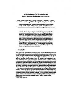
Figure 1: A screenshot of the user interface of our implementation of Dominion. Cards tinted with green are those which can be played during the current phase. During the buy phase, the cards in the supply that the player can afford are also tinted green.

The players will start by drawing seven Copper cards, the cheapest treasure card, and three Estate cards, the cheapest victory card, from the supply – these cards form the players’ starting decks. The starting decks are shuffled and each player draws five cards. A predetermined starting player2 plays a turn, after which the turn passes to the player to the left until the game has reached one of its ending conditions. When playing a turn, a player goes through three phases: Action Phase: During this phase the player has one action, which can be used to play one action card from her hand. The player may gain further actions from the action card played initially, which can in turn be spent on playing more action cards subsequently. Buy Phase: During this phase the player can play treasure cards to gain coins, which are added to any coins gained by playing action cards during the action phase. These coins can be spent on buying the cards in the supply. The player has one buy available each turn, which means that she is allowed to buy one card that she can afford. Many action cards increase the number of buys that the player can make, which allows the player to split her coins on multiple purchases. The cards bought are put into the player’s discard pile. Clean-up Phase: In the clean-up phase the player discards all cards played in the previous two phases along with any 2 Chosen randomly for the first game, and chosen as the player to the left of the last game’s winner for subsequent games

3.1 dominion

Figure 2: Examples of the card types (Curse excluded) – victory, treasure and action, respectively. The cost of a card can be seen in its lower left corner. The particular action card, Market, allows the player to draw one card and gives her one more action. Furthermore, it gives her an extra purchase in the buy phase, and one extra coin to spend.

cards left in the hand. The player then draws a new hand of five cards from the deck (should the deck run out of cards, the player shuffles her discard pile and places it as her new deck). The turn then passes to the player on her left The game ends if, at the end of any player’s turn, either or both of two requirements have been met: • The stack of Provinces (the most expensive victory card) is empty. • Three of the stacks of cards in supply are empty. Once this happens each player counts the number of victory points among her cards, and the player who has gathered the most is the winner. Should two players have the same number of victory points, the player who played the fewest turns is the winner. Should the players also draw for the number of turns, the players share the victory. Some of the action cards are attack cards as well – this means that they negatively influence opponents on top of any positive effects they might have for the player playing the card. These negative effects can be countered if the player who would be affected can reveal a reaction card (another subset of action cards) from her hand3 . For a list of the cards and their rules see Appendix C. The shuffling of the decks makes Dominion a non-deterministic game. Players have limited information (the order of the cards in 3 The only reaction card in the basic Dominion game is Moat. More reaction cards have been introduced in expansion packs.

9

10

the game

their own decks as well as the contents of the opponents’ hands, decks and parts of their discard piles are all unknown to the player). The game is also a nonzero-sum game. Dominion does not necessarily terminate – should all the players decide not to buy any cards, the game will go on for ever. As argued by Pollack and Blair (1998), some games involving a degree of randomness have an inherent reversibility, i.e. the outcome of the game continues to be uncertain until some point. As players have non-trivial chances of winning or losing up until this point, the players can potentially learn from each move, which makes the domain particularly suited for co-evolution. Other domains will punish blunders early in the game so severely that learning from each move will be unlikely, as the game is already virtually decided. Dominion is likely closest to the latter category, as the options available to a player are determined by her own choices in earlier turns, as well as the choices made by opponents (if, for instance, the opponents use a lot of attack cards or buy all the cards in a specific category). The cards acquired early will be likely to show up the most times during a game, so a bad decision made early will be haunting the performance of the player’s deck more than one made late in the game. 3.2

assumptions and premises

Often, when attempting to apply machine learning techniques to create an agent for a game, the game is simplified to some degree. Many machine learning approaches to finding solutions to games, which are actually played by human players, simplify these games almost beyond recognition. We have attempted to make as few changes to the rules of Dominion as possible (if too many rule modifications are needed one might argue that selecting a simpler or more appropriate game would have been prudent). Some changes to the rules have been made though, which are described in the following. 3.2.1

The cards

Dominion has 32 different cards with a wide range of different effects on the game. It would no doubt be easier to train an AI to play well using a subset of these 32 cards. We did, however, consider it feasible to implement all 32 and to train the AI using the full set of cards, and as we consider a general solution more interesting than a solution to a single configuration, or to a smaller subset, we decided to implement all the cards.

3.2 assumptions and premises

A number of expansions and promotional cards have been published for Dominion. We have chosen to not include these in our experiments, as we did not have access to neither the expansions nor the promotional cards, and as implementing these would require a lot of work not directly related to the application of machine learning. 3.2.2

The number of players

The basic Dominion game is played by two to four players. We elected to always use four players for training and testing purposes. This decision was made because we did not want to introduce a changing number of players as another factor agents would have to take into account when training. We chose four players, rather than two or three, as having to deal with three opponents would likely be a more interesting problem to solve, and as we personally consider the four player game the most interesting to play. 3.2.3

Winning conditions and end game

As stated in 3.1, should multiple of the highest scoring players have the same number of victory point and have gained these in the same number of turns, these players share the win. This turned out to be impractical when running batches of many games, as which player wins determines who will start the next game. In order to properly find a starting player in such a way that the advantage of starting would not be given to a particular position, we elected to randomly select a winner among the players who would otherwise be sharing the victory. As mentioned in section 3.1 Dominion is not guaranteed to terminate. When it does not terminate (or when it takes a very long time to terminate because players are reluctant to buy cards) it is a sign that the four players participating are unskilled. Observing players in early evolution we found that an unreasonable amount of time was being spent on evaluating players who were not skilled enough to actually buy cards. As we estimated that these games would not be likely to contain very important genetic material we simply elected to end the game after 50 turns and tally the score as if the game had ended by either of the two conditions having been fulfilled. The various agents will not attempt to analyze the outcome of making a move before they make it. This means that no prediction of whether emptying a certain stack of cards will terminate the game will take place, nor of whether this will make the player win

11

12

the game

or lose. This is of course limiting for the agents’ ability to play, but as it would be somewhat unrelated for the learning of Dominion strategies we decided not to introduce special handling of the end game (section 8.3 contains a brief description of how this might be implemented). 3.3

approach

The decisions needed for playing the three phases of a turn in Dominion are vastly different (see section 3.1 or Vaccarino (2008) for a more thorough description of the phases). In the action phase the player must make decision on which of the action cards in hand to play, and in which order. Some decisions here are fairly straightforward. For instance, if the player holds a Village card and a Smithy card, playing the Smithy card first would leave the player with three newly drawn cards whereas playing the Village card first would have the player holding four newly drawn cards and have one action left, which could again be used to play any action cards drawn. Other decisions are more difficult – would it be best to play the Militia card to get two coins and potentially hamper the hands of the opposing players or should one rather forgo the chance to disrupt the opponents’ hands and play a Smithy card to draw three cards, in hope that these will have more coins than the Militia card would provide? The choices a player must make during the buy phase are central to the future performance of a player’s deck. Which cards the player buys during the buy phase determine which cards she will be able to play in later action phases, how many coins she has available during the buy phase, how many victory points she will have at the end of the game and even whether she will be able to defend herself against attack cards played by opposing players during their turns. It is quite obvious that the skill of a player in Dominion is highly dependent on the strategy employed when selecting cards to gain. It would appear that, though both are required to achieve good play, the decisions made during the action phase and those made in the buy phase are widely different. For this reason we have elected to split the solution into two distinct parts, one which is tasked with handling the action phase and another one which handles the selection of which cards to gain. There are overlaps between the action and the buy phase – it is possible to gain cards during the action phase (for instance

3.3 approach

when playing a Feast or a Remodel). If such a card gain involves a choice between gaining different cards the choice will be made as if it were the buy phase. The clean-up phase is mainly a question of administrating the end of the turn: Cards which have been played during the turn and cards left in the player’s hand have to be discarded, the player must draw a new hand and so forth. Actually only one decision can be made during the clean-up phase; the order in which to discard the cards from the player’s hand. The cards which have been played during the turn go into the discard pile first and these will all have been seen by the opposing players. The cards in the hand have not, so the player has the option of hiding some of the cards in hand from the opponents by discarding another card as the very last4 . To avoid taking opponent modeling (Schadd et al., 2007) into consideration to obtain a marginal improvement at best, we have decided to merely let the choice of which card to discard last be made at random. Dominion is designed so that cards which influence whether or not the player is winning (victory cards and curse cards) are not useful during the actual playing of the game5 . Therefore a human player, when faced with the option of gaining a card to add to her deck, would make a choice between the available cards in part based on an estimate of how progressed the current game is. If she estimates that the game is currently in an early phase, she can expect that the bought card will show up in the hand a larger number of times than a card bought later in the game. As decks as a rule grow in the course of a game, a card gained during the early game will also constitute a larger percentage of the deck in the immediately following turns. Hence, buying a victory card early, while giving the player a head start in terms of victory points, will also greatly hamper the player’s deck and reduce the chance the player will get of gaining more and higher value victory cards later in the game. Likewise, choosing an action or treasure card over a victory card in the last turns of a game would only rarely have a significant positive impact on the player’s performance: the action or treasure card would not likely come into play, and even if it did so, no more than a few times; only in rare instances could it prove more beneficial towards the player’s total number of victory points than the victory card would. 4 It could for instance be advantageous to hide a Moat card so that the other players will not know how many of your moats are in the discard pile and then in turn will not be able to discern whether you might have one in hand. 5 They can neither be played during the action or buy phase and with certain cards in play (Bureaucrat) having one in hand even constitutes a risk.

13

14

the game

A problem with many of the basic strategies we have encountered6 is that they often have a notion of ‘early’ and ‘late’ game without being able to specify what these vague terms correspond to in terms of the actual game state. Is it a late game state when there is only a specific percentage of the starting provinces available, and is this to be considered more or less late game than when some of the supply stacks are nearly empty? It is easy to come up with experience-based heuristics in reply to questions like that, but the result will hardly be very general or optimal. We believe that having a way of estimating the progress of a game of Dominion is essential to playing the game. To avoid vague heuristics based on expert knowledge, we decided to use machine learning for a separate part of the player, tasked solely with estimating a game’s progress depending on the game state. We intend to use these estimates of the game’s progress for the other two parts of the solution. Some decisions are unrelated to buying or playing cards – the decisions of whether or not to reveal a Moat when faced with an attack card or put a particular card aside when playing a Library are examples of such. These decisions have to a high degree been left to heuristics – see Appendix A for a complete list.

6 See for instance Boardgamegeek (2008).

4

METHOD

In our attempt to create a powerful agent for Dominion we have used several techniques, most of which will likely be familiar to those who are experienced in machine learning. As a reference to those readers who are, and as an introduction to other readers, they are described in relative brevity in this chapter. 4.1

artificial neural networks

The human brain consists of nerve cells (neurons). Each neuron is connected to a number of other neurons and each neuron can transmit information to or receive information from the connected neurons. These complex networks are believed to be the foundation of thought (Russell and Norvig, 2003, pp 10-12). In attempting to create artificial intelligence one approach would be attempting to simulate the cells in the human brain, which was first done by McCulloch and Pitts (1943). The simulated neurons (often called nodes or units) receive a number of inputs through a number of connections (often also referred to as links). Each connection has a weight associated with it, so that the sum of the inputs to the node can be considered a weighted sum (Russell and Norvig, 2003, pp 736-748). The output, y, of a node depends on this weighted sum as well as the node’s activation function, g, and is written as

y=g



n

∑ wi · x i



(4.1)

i =1

where xi and wi represent the ith input and weight respectively and n is the number of inputs to the node. It is obvious that the activation function is important for the output. Among the most commonly used are the threshold function or step function, which outputs 1 if the weighted sum of the inputs is zero or higher and otherwise outputs zero, the linear activation function, and the logistic sigmod-shaped activation function (henceforth sigmoid function):

g( x ) =

1 1 + e−Sx

(4.2)

15

16

method

S being the slope parameter (henceforth just referred to as slope) of the sigmoid activation function. The advantage of the step function and the sigmoid function is that a relatively small change in the weighted input sum can result in a relative large change in the output in some situations (when the weighted input sum is close to the ‘step’ of the threshold function or the steepest slope of the sigmoid function) while in other situations (when the weighted input sum is not close to the ‘step’ or steep slope) the change in the output will be small. Some methods of learning requires the activation function to be differentiable (see section 4.2), which puts the sigmoid and the linear activation functions at an advantage. Many nodes have a constant input called the bias. As the bias does not change, the weight on the connection leading it into the node can be considered defining the placement of the step of the threshold function or the steepest part of the sigmoid function. The value of the bias input is often set to −1. Such nodes connected to each other is called an artificial neural network (henceforth neural network). If there are no cyclic connections in the network it is called a feed-forward network and if it has cyclic connections it is called a recurrent network. The nodes of feed-forward networks are often organized in layers, so that the (weighted) outputs from one layer is fed as inputs to the nodes of the next layer. A layer which is composed of neither input nodes nor output nodes is called a hidden layer, and the nodes in it are called hidden nodes. If we consider a network composed of a single node (often called a perceptron) using a step function, this node will define a hyperplane dividing the search space (which has a dimensionality equal to the number of mutually independent inputs) in two, a part where the output of the perceptron is one and another where it is zero. To see that this is a hyperplane, consider when the threshold function will activate: ∑in=1 wi · xi > 0 – this splits the space in two by the hyperplane ∑in=1 wi · xi = 0. For problems that are not linearly separable one would need to arrange nodes in multiple layers. For a better, smoother function approximation, one might use the ‘softer’ sigmoid activation functions. 4.2

backpropagation

Backpropagation is a technique with which the weights of a neural network can be optimized in order to make the neural network deliver certain outputs for certain inputs, or more precisely: “The

4.2 backpropagation

aim is to find a set of weights that ensure that for each input vector the output vector produced by the network is the same as (or sufficiently close to) the desired output vector” (Rumelhart et al., 1986). The technique, which was first described by those authors, is outlined in the following (index letters have been changed for readability). For backpropagation to work, one must have training data – a set of inputs and the outputs relating to them. The neural network should also be a feed forward network without recurrency. By presenting a neural network with this input data one can calculate an error:

E=

1 ∑ (a j,c − d j,c )2 2∑ c j

(4.3)

where c is the index of the elements in the training set, j is the index of output units and a j,c and d j,c are the actual and desired output for this output unit and training set. Recall that the input to a unit, q, is a linear function of the outputs, y p , of the units connected to it and the weights of those connections (w pq ). The input, xq , can then be written as

xq =

∑ y p · w pq

(4.4)

p

and that this, if using a sigmoid activation function, is routed into the activation function to produce an output for the unit (see equation 4.2), so the output is:

yq = g( xq ) =

1 1 + e−Sxq

(4.5)

To minimize E we can compute the partial derivatives of E for each weight in the neural network, then use these derivatives to modify the values of the weights. For the output units this is straightforward – one simply differentiates equation 4.3, which (for a single input/output pair) yields ∂E = yq − dq ∂yq Applying the chain rule to find ∂E ∂E ∂yq = · ∂xq ∂yq ∂xq ∂y

(4.6) ∂E ∂xq

we find (4.7)

To find ∂xqq we differentiate equation 4.5 (considering S = 1 for simplicity) which (along with equation 4.7) gives us an expression

17

18

method

for how to change the total input to the output unit in order to change the error: ∂E ∂E = · y q · (1 − y q ) ∂xq ∂yq

(4.8)

This is needed for the computation of the derivative of the error with respect to a certain weight: ∂E ∂xq ∂E ∂E = · = · yp ∂w pq ∂xq ∂w pq ∂xq

(4.9)

So now, for an output node q, given the actual and desired output and the output of a previous unit p we can compute the partial derivative of E with respect to the weight of the connection from ∂E p to q: ∂w . For a unit, p, connected to q the error from the output pq unit can be propagated back: ∂E ∂E ∂xq ∂E = · = · w pq ∂y p ∂xq ∂y p ∂xq

(4.10)

If node p is connected to multiple output units, this can be summed to ∂E = ∂y p

∂E

∑ ∂xq · w pq

(4.11)

q

These steps can be repeated, propagating the error back through ∂E the neural network. Now we have an expression for ∂w for each weight in the network. These can be used to compute changes to ∂E the weights: ∆w = −e · ∂w , e being a small constant, the learning rate. 4.3

neat

When NeuroEvolution of Augmenting Topologies (NEAT) was first introduced by Stanley and Miikkulainen (2002c), it was shown to outperform earlier techniques on the benchmark of double pole balancing (see Barto et al., 1983, for a description of the benchmark and its justification), by a large margin1 . The factors behind this significant success were threefold, as was shown by the ablation studies following the initial benchmarks. • First, instead of starting with a fixed topology and only evolve the connection weights, NEAT allowed the networks to complexify over the course of evolution. 1 NEAT beat the previous record holders, Cellular Encoding and Enforced Subpopulations, by factors of 25 and 5, respectively (Stanley and Miikkulainen, 2002c)

4.3 neat

• Second, NEAT would start from a minimal topology consisting of only the input nodes with full connections to the output node. This, it was argued, allowed the search for optimal weights to be performed in a smaller number of dimensions, allowing for better weights to be found. • Third, the concept of speciation was used to protect new innovations, to allow them to evolve their weights without becoming extinct too fast for the effectiveness of their topology to be tested properly. Earlier experiments in neuroevolution had used fixed topologies containing a varying number of hidden neurons, layers and connections. These parameters had to be decided upon, and experienced users of machine learning will most likely know and agree that this parameter selection can be time consuming and tedious, since it often ends up as a trial and error process. All the aforementioned factors were strongly dependent on the novel concept of historical markings in combination with the genetic encoding employed by NEAT. The genes of NEAT can be split into node genes and connection genes. The first contain information on the input, hidden and output nodes, while the latter hold information on each connection, its weight and the historical marking in the form of an innovation number. Two kinds of mutations can happen in NEAT. The mutation on weights is the simplest of these, in that it occurs in much the same way as in other neuroevolutionary systems; with a certain probability, the connection weight will either be perturbed by a small random amount, or it will be set to a new random value in the interval allowed for weights. The more complex mutation is that of the topology of the neural network, which may occur in two different forms: The addition of a new connection or a new node. The first will select two random neurons that thus far have been unconnected, and add a connection between them. This new connection gene will receive an innovation number which is simply the previously highest innovation number incremented by one. The latter will select a random connection to be split into two connections, with a new node between them. These new connections will each receive a new innovation number, in the same way as with the add connection mutation. As these innovation numbers are inherited, NEAT always keeps track of which connection genes stems from the same topological mutation. When genomes are to be crossed over during mating, they utilize the innovation numbers in the connection genes to line up those

19

20

method

genes that share historical origin. Crossover in the form of random selection from either parent is applied for all the genes that match up, while those that do not match up are selected from the more fit parent. The historical markings also provide the basis for speciation, which NEAT employs to ensure diversity in the population. When comparing genomes, some genes will inevitably not match up. These are either disjoint, when the innovation number is within the range of those of the other parent, or excess if they are outside that same range. The count of disjoint and excess genes are used to measure the distance between two genomes, when deciding whether they belong to the same species. The distance δ between two such genomes is

δ=

c1 E c2 D + + c3 · W, N N

(4.12)

where E and D are the numbers of excess and disjoint genes, respectively, and W is the average distance between the weights of the matching genes. Three constants, c1 , c2 and c3 are selected by the user to specify the importance of each of the distance measures. N is the size of the largest of the two genomes being compared, effectively normalizing δ by the genome sizes. When species are decided upon, each genome after the first (which automatically ends up in the first species) is compared to a random member of each species until the distance between the two is below a threshold selected by the user; the genome is assigned to the first species it is sufficiently close to, or to a new species if it is too distant from the other species. Once this has been done for all the genomes, they have their fitness for selection purposes adjusted relative to the size of their species, in that each of their individual fitnesses are divided by the count of members of their specific species. This is also known as explicit fitness sharing where, as phrased by Rosin and Belew (1995); “An individual’s fitness is divided by the sum of its similarities with each other individual in the population, rewarding unusual individuals.” Each generation, when genomes are selected for survival due to elitism, the speciated fitness will ensure that a diverse population is maintained, by eliminating the less fit members of each species first. When topological mutations occur, chances are that the newly added structure will cause a drop in the fitness of the newly created genome, compared to previous, smaller ones (Stanley, 2004, section 2.5). New genomes with an innovative topology are protected by their small species sizes, and the less fit genomes

4.4 competitive co-evolution

in larger species will be eliminated first. Therefore innovative mutations will have the time needed for their connection weights to be optimized, and the fitness of their topology to be fairly tested. 4.4

competitive co-evolution

Co-evolution in genetic algorithms was first suggested by Hillis (1990). It is a technique by which multiple genetically distinct populations with a shared fitness landscape evolve simultaneously (Rosin and Belew, 1995)2 . The term competitive signifies that the individuals in the populations being co-evolved have their fitness based on direct competition with individuals of the other population. The advantage of co-evolution is that it creates an ‘arms race’ in which one population (traditionally called the host population) will evolve in order to surpass test cases from the other population (called the parasite population). The roles are then switched so that the population that was previously the parasite becomes the host and vice versa. Competitive co-evolution has been shown to achieve better results than standard evolution, to achieve these results over fewer generations and to be less likely to get stuck at local optima (Lubberts and Miikkulainen, 2001; Rawal et al., 2010). 4.4.1

Measuring evolutionary progress

The shared fitness landscape of competitive co-evolution makes it difficult to measure evolutionary progress (Cliff and Miller, 1995). Comparing solutions across generations is no longer straightforward as the fitnesses of these solutions are relative to the test cases chosen from the other population. With an exogenous fitness, a ranking of two agents could be performed by merely comparing their fitness scores, but with relative fitnesses this is not an option. Furthermore, for complex games like Dominion, the evolution might get stuck in a ‘strategy loop’, in which a population will lose the ability to exploit a certain weakness if this particular weakness does not occur in the opposing population any longer (Cliff and Miller, 1995; Monroy et al., 2006). The opposing population might then develop the same weakness, which would force the first population to re-evolve the ability to exploit this and once again weed out the opposing players having this weakness. To an observer watching the champions getting replaced by new 2 Co-evolution is also sometimes attributed to Axelrod (1987), but while it is competitive evolution with a shared fitness landscape, it only utilizes one population, which sets it apart from what we mean by competitive co-evolution.

21

22

method

champions, this circularity might look like evolutionary progress. A method of monitoring progress that has often been used is the hall of fame as suggested by Rosin (1997). The hall of fame stores the best performing individual from each generation in order to use them to test members of populations in later generations. The members of the host population will be tested against not only members of the parasite population but also against some selection of the members of the hall of fame3 . If we wish merely to monitor the progress of the evolution, a master tournament as suggested by Floreano and Nolfi (1997) can be used. A master tournament is simply testing the best performing individual of each generation against the best performing individuals of all generations. With a large number of generations and a large amount of games needed to accurately detect differences between these ‘master’-individuals, such a tournament might take quite a while. Stanley and Miikkulainen (2002b) further argues that a master tournament does not indicate whether the aforementioned ‘arms race’ takes place – it merely shows if a champion can defeat other champions, but does not show strategies defeating other strategies and is therefore not capable of showing if the evolution has gotten stuck in a loop. Instead Stanley and Miikkulainen (2002b) suggest a dominance tournament, in which each generational champion is tested against all other previous dominant strategies. The first generational champion becomes the first dominant strategy outright. If a generational champion later manages to beat every previous dominant strategy it becomes a dominant strategy itself, and future dominant strategies must be capable of beating it. To limit the amount of games needed, the candidate plays the opponents in the order last to first – that is, hardest to easiest – and the tournament terminates if it fails to beat any opponent. As a generational champion will only be required to play against a subset of the previous champions, and as this tournament can often be terminated early, a dominance tournament is much less computationally expensive than a master tournament. It is also a handy tool for tracking evolutionary progress, as any strategy added to the collection of dominant strategies will be known to be capable of beating each previous dominant strategy.

3 Rosin (1997) suggests random sampling if re-evaluating the fitnesses of the members of the hall of fame will be time consuming, which would likely be the case for Dominion-agents.

4.4 competitive co-evolution

4.4.2

Sampling

Having every member of one population play against every member of the opposing population in order to measure fitness values is computationally expensive – as argued by Rosin (1997): “It is desirable to reduce the computational effort expended in competition by testing each individual in the host population against only a limited sample of parasites from the other population”. The questions remain which opponents to pick from the parasite population, and how to pair them up with the members of the host population. As the competitions are held to find a relative fitness hierarchy of the members of the host population, each host must compete against the same selection of opponents – if playing against different samples of the parasite population a host might get an unrealistically high fitness from playing against comparatively weak opponents. Let us address the question of how to play these games before getting into whom to play them against. Many games used as benchmarks for competitive co-evolution are two player games, and it would appear that not much research has been done on how to deal with games with higher numbers of players, so a brief discussion is in order. One could potentially match one host against one parasite in a series of games – as we are not dealing with less than four players (see section 3.2) this could be done by including two instances of the host player and two instances of the parasite player in the same game. While this would ensure an even match between the two, more similar series of games would be required to make sure that the hosts’ fitness values are based on a diverse selection of opponents. Another option would be matching two instances of the same player against two different members of the parasite population. This would have a better diversity, but it might favor strategies based on ending the game quickly, as the two identical players would be able to support each other effectively by buying the same types of cards and thereby closing the game faster. This could be avoided by playing two members of the hosts population against two members of the parasite population. It would not mean that we could evaluate the fitness of twice as many hosts per game though, as we still need the hosts to have played against the same opponents in order to create a fitness hierarchy – one of the members of the host population would need to be present in all games. Furthermore this member of the host population would also need to be tested – as it would need to play against the same players as each of the other members of the host population it would end up playing against itself, which again

23

24

method

would favor strategies based on closing the game fast. This would also change the nature of the fitness landscape of competitive co-evolution, the consequences of which are difficult to foresee. Instead we opted for matching one member of the host population against three different members of the parasite population. While we are only testing one member of the host population at any given time, this matching can be used to test against diverse opponents while not favoring any particular strategies. Now it remains to find the members of the parasite population that each member of the host population should be competing against. One option would be picking random players. This would sometimes result in the hosts being faced with relatively weak competition if only unskilled members of the parasite population are chosen, which would mean a loss of the ‘arms race’ edge of competitive co-evolution (Monroy et al., 2006). As stated by (Stanley and Miikkulainen, 2002a): “The parasites are chosen for their quality and diversity, making host/parasite evolution more efficient and more reliable than random or round robin tournament.”. In order to get the highest level of quality we could use the champions, and to get a diverse sampling we could pick members of different species. Combining these, we use the champions of the three best performing species of parasites. Should less than three species occur in the parasite population, the best performing champion is used to fill in any gaps – this situation will only rarely arise when adjusting speciation parameters on the fly in order to make sure the populations have a certain number of species (an addition to the original NEAT, see Stanley, 2010). 4.4.3

Population switches

As mentioned competitive co-evolution is created to sustain an ‘arms race’ between the two populations – the idea is that if both populations evolve, they will be fairly evenly matched and a good choice for evaluating the fitness of the opposition. The question of when to evaluate (and evolve on) one or the other population is largely unexplored though. Stanley and Miikkulainen (2002a) state that “In each generation, each population is evaluated against an intelligently chosen sample of networks from the other population” i.e., both populations are subject to evolution in each generation. Many other texts on co-evolution do not touch upon the topic of population switches (Rosin and Belew, 1995; Floreano and Nolfi, 1997; Rawal et al., 2010, just to name a few) and one must assume that they are using the ‘standard’ version of evolving: evolving on both populations in

4.5 monte-carlo-based approaches

each generation. This method of switching population seems somewhat in conflict with the ‘arms race’ purpose of competitive co-evolution. In order to force either population to improve one would assume it would be best if it is faced with a population of slightly higher skill. If assuming that one population is more skilled than the other, one must necessarily be playing against a population less skilled than itself when the standard competitive co-evolution lets both populations be evaluated by playing against the other. With proper sampling (see section 4.4.2) the individual competitions might not be played against less skilled players, but the question remains: is this evolution worth the computational effort spent on it. As approximately half the computational effort goes into training populations which are already doing better than their counterparts, one could reach twice the number of generations if only evolving on the least skilled population. This might mean that when only the worst performing population is evolved, the ‘arms race’ ability of competitive co-evolution has a larger impact as it is present in every generation. One might, however, also imagine that an unreasonable amount of time gets used on evolving on an inferior population, while the better population is not evolving, which could mean that the solutions found would be less skilled. A third option would be that the method chosen for population switches is unimportant so that the skill of the evolved individuals will not be influenced by this. The unforeseeable effects of making changes to the populations switches of NEAT, as well as the apparent lack of research done on the subject, made the question of different methods of population switches interesting to us. We intend to use Dominion as a testbed for comparing these two approaches to population switches in competitive co-evolution, which we call switch by skill (by which we mean only evolving on the population that has the lowest skill) and switch by generation (evolving on both populations every generation) – see section 6.2.3. 4.5

monte-carlo-based approaches

Since some Monte-Carlo approaches have served as inspiration during the course of our studies, we give a brief description of those in the following. Monte-Carlo Tree Search was presented in 2006 by Chaslot et al. (2008), and has shown great promise in computer Go (Lee et al., 2009). The algorithm builds a tree of possible states from the

25

26

method

current one, and ranks them according to how beneficial they are judged to be. The tree starts out with only one node, corresponding to the current state. A tree of possible subsequent states is then built by repeating the following mechanisms a number of times, as described by Chaslot et al. (2008): Selection If the game state is already in the tree, the inferred statistics about future states are used to select next action. Expansion When a state is reached that does not already have a corresponding node in the tree, a new node is added. Simulation Subsequent possible actions are then selected randomly or by heuristics until the end state is reached. Backpropagation Each tree node visited is updated (i.e. the chance of winning is re-estimated) using the value found in simulation. After the algorithm has run the desired number of simulations, the action corresponding to the node with the highest value is selected. Another variant of Monte-Carlo-based search is the one using UCB1 (Auer et al., 2002) employed by Ward and Cowling (2009). Instead of building a tree like in MCTS, it relies on random simulation of possible actions after all actions directly available from the current state. The action to be simulated is selected based on the average rewards from actions found by earlier simulations (the algorithm is initialized by simulating each action once), plus a value calculated from the number of times the actions have been simulated. That is, the action j that maximizes s xj + C

ln n nj

(4.13)

is simulated, where x j is the average reward of previous simulations of the action, C is a constant in the range [0, 1] controlling exploration/exploitation (with larger values corresponding to more uniform search), n j is the number of times the action has been simulated, and n is the total amount of simulations that has been performed. 4.6

tools

A working digital version of Dominion was implemented in Java. The interface was created using Slick, a software package for creating 2D-graphics in Java (Glass et al., 2010). Training of neural networks using backpropagation was done using a modified

4.6 tools

version of Neuroph, which is a neural network framework for Java (Sevarac et al., 2010). The training of neural networks using NEAT was done in a modified version of ANJI (Another NEAT Java Implementation by James and Tucker, 2010).

27

5

P R O G R E S S E VA L U AT I O N

As argued in section 3.3, an estimate of how long the game will last is important for many of the decisions that a player needs to make in order to play Dominion well. This section describes the choices and observations made in creating progress evaluation for Dominion. 5.1

method

What is really needed is a continuous estimate of game progress, as opposed to discrete notions of ‘early’, ‘middle’ and ‘late’ game. This can be achieved in a number of ways. One might do a simple weighted sum of parameters deemed relevant to the estimation of game progress, or the same parameters might be used as input for a neural network approximator. The decision to use a neural network for this part of the AI seems an obvious one: Neural networks have shown their worth countless times1 in providing approximations of complex functions of a number of numerical values based on properly preprocessed inputs. As the game’s turn progress can be seen as a real number within [0, 1] ( max turn ), and all the relevant input can be normalized to that same interval, plugging things into the neural network, as well as putting the output to use is an easy task. The question of how to train the neural network now remains. One approach could be evolving a neural network using NeuroEvolution of Augmenting Topologies (NEAT). NEAT is at an advantage for problems where a complex topology is needed in order to get a good solution. It can, however, be quite cumbersome, with many parameters to set and very few guidelines as to how to set them. As NEAT is a randomized approach, a significant amount of computational effort will also be spent on evaluating solutions of lower fitness than previous ones. turn As we have a desired output (the value of maxturn , which is stored when training data is produced) as well as an actual output, using backpropagation would also be an applicable way of training the neural network. Backpropagation is fast and reliable, but can be hampered by local optima.

1 Among the most well-known within the AI community is Tesauro (1995)

29

30

progress evaluation

Because we do not consider it likely that a complex topology is needed, and do not consider progress prediction in Dominion to be a problem which would likely have many local optima, we have opted for using backpropagation in our training of the neural network. For either of these techniques to work, decisions have to be made regarding which parts of the game state are relevant. The choices we have made are discussed in the following. 5.1.1

Representation

As mentioned in section 3.1 a game of Dominion can end in one of two ways, which we recall to be: • Three of the supply stacks are empty at the end of any player’s turn • The stack of provinces is empty at the end of any player’s turn This suggests that the number of provinces left is important to the estimate of the game’s progress, as well as the number of cards in the three supply stacks with the fewest cards left in them. Such an approach is not particularly fine-grained though: for instance it would make a situation with two empty and one nearly empty stack indistinguishable from a situation with two empty and two nearly empty stacks. From the player’s point of view these situations could be very different, as the latter might offer an opportunity for closing the game cheaper or with a higher victory point gain than the first one. Therefore we decided to include the number of cards in the four lowest stacks in our initial selection of the inputs to the neural network. The number of provinces left and the nearly empty stacks might not be sufficient information about the game to predict when it will end: In some games the selection of kingdom cards means that the players will get enough money to buy the more expensive cards early, while in others, scraping together enough coins to get the right cards can be difficult. Also, in some games the selection of cheap cards may be large while in other games these might be rare (this influences whether players can end the game with relatively weak economies or not). Therefore, the costs of the cards in the four smallest stacks would be meaningful to include as a part of the game state useful for predicting progress. This leaves the amount of coins the players are able to spend which, like the cost of the cards, influences how fast a game can

5.1 method

be closed. This could be represented in a number of ways – for instance the average ratio of coins per card in a player’s deck or the number of coins the player used during the previous buy phases. These approaches both suffer from an inability to recognize certain strategies though: For instance, if a player forms her deck around gaining cards costing four coins by playing Workshop cards, and then using Remodel cards to turn these into cards costing six coins and later to cards costing eight (i.e. Provinces), the potential of her strategy will not be recognized by examining the cards gained during the buy phase or the average coin value of her deck. Therefore, using information about the gains made during a turn (during the action and buy phases) will give a more accurate picture of the card gaining potential of a deck than merely looking at the treasure cards in the deck or the buys made will. As we estimated that remembering only one turn could give very unreliable results (as the opposing players might have drawn particularly weak or strong subsets of their decks) we elected to measure the average of the best gains over a number of turns. We average this over three turns – four or five would give us a smoother curve of buy averages over turns (which would also mean that the impact of players’ particularly lucky or unlucky turns would be diminished), but it would also be less sensitive to changes in the buy/gain-power of decks. Comparing agents using averages over different numbers of turns might reveal which choice is better. This, however, is beyond the scope of this thesis. So, to summarize, these are the inputs we have chosen for our neural network: Lowest stacks The amount of cards left in the supply stacks closest to being empty. This input appears four times, once for each of the four stacks with the fewest cards in them. These inputs are normalized through division by the total number of cards of the given type at the start of the game. Lowest stack costs The costs of the cards in the stacks closest to being empty. Like the lowest stacks, this input appears four times. The lowest stack costs are normalized through division by eight, as this is the cost of the most expensive card in the game. Gain average The average gains of the players, averaged over three turns. This value is normalized by eight as well. Provinces The number of provinces left in supply, divided by the total number of provinces in the game2 for normalization. 2 12 in our case, as we play only four player games.

31

32

progress evaluation

Bias (1) 5.2

experiments

Though the training of a neural network might seem a fairly automated process, there are some parameters that still need to be decided upon. The most important of these is the error function, which is described in section 5.2.1. We also had to decide upon an activation function for the output node and the nodes in the hidden layer of the neural network. As we wanted a gradual change in the estimates of progress, using a step function was out of the question. Linear and sigmoid activation functions would both be able to give us this gradual change – we eventually decided on a sigmoid activation function, as this would allow for small changes in inputs to a node to result in large changes in the output, which we believe would be advantageous in the training of progress prediction Dominion. We used a slope of S = 1, as this is also the default value used by Neuroph (see section 4.6). 5.2.1

Error function

We wanted an error function which would attribute the lower error values to networks which made estimates of progress close to the actual progress:

Egame =

∑tT=1 E(t) T

(5.1)

Here Egame is the error of an agent’s prediction of the progress over an entire game lasting T turns, with E(t) being the error for the prediction of the progress for a single turn, t. The same approach can be used to compute the average error for a collection of turns that is not a game (this could for instance be a series of games) by merely considering T the total number of turns in the collection. If instead of defining t as the turn, we define it as the current turn divided by the total number of turns, we can define our desired output as a function of t, namely D (t) = t. Given the actual output of the neural network approximator, A(t), we can define an error for the progress prediction in a single turn to be

E(t) = | D (t) − A(t)|

(5.2)

5.2 experiments

This error in the prediction for a single turn, E(t), is between 0 and 1. The higher values can only be achieved during late or early game, and halfway through the game the error function for the turn can at most be one half. As the maximum error is linear both in the [0, 12 ] and the [ 21 , 1] interval, the highest average error that progress prediction can get for an entire game is 0.75 (see figure 3).

Figure 3: The maximum error as a function of game progress.

If our output node of the neural network is unconnected (i.e. all the inputs to the output node will be zero), the output will be 0.5 for every input (see equation 4.2), the actual output, A(t), being A(t) = 21 . As we have negative as well as positive weights, this is somewhat similar to initializing the neural network with random weights between −1 and 1 3 , which will yield outputs averaging 0.5. Using this A(t), our error function is 1 E(t) = | D (t) − A(t)| = |t − | 2 The integral of this function, average error of the output, is  Z t  1 t (1 − t ) if 0 ≤ t ≤ 12 , E(t0 )dt0 = 2 1 2 1 0 4 (2t − 2t + 1) if 2 ≤ t ≤ 1. 3 Or between any number and minus the same number

33

34

progress evaluation

For the t = [0, 1] interval (an entire game) the average error is: Z 1 0

5.2.2

E(t0 )dt0 =

1 4

Producing training data

In order to train a neural network to evaluate the progress of a given game by looking at the subset of the game state described in section 5.1.1 we needed to gather such subsets for a large number of games. Rather than having four human players spend enormous amounts of time playing the game, we decided to make a finite state machine player (henceforth FSMPlayer) capable of playing the game following simple heuristics. As different kingdom card configurations might make games very different in terms of play time, we decided to create training data using random selections of kingdom cards. Using one subset of the kingdom cards to train would likely create a very good solution for that particular set of card while not yielding a good general approximation of game progress. The series of games were played using the rules for restarting the game (see Vaccarino, 2008) – this means that the winning player of one game will be playing last in the following game and thereby be at a disadvantage. This diminishes the impact of the slight advantage a starting player has – if one player is significantly stronger than the other players though, the player to the left of the strong player could have a minor advantage compared to her peers. 5.2.3

Finite state machine player (FSMPlayer)

This finite state machine (henceforth FSM) considers the game in one of three states; early, mid-game or late. The transitions between these states are simple, expert knowledge based heuristics – for instance the game is considered to no longer be in the early state once the first province has been bought by a player, if the first stack is entirely empty or when the sum of the number of cards in the three smallest stacks drops below 13. The value that the FSMPlayer attributes to gaining a card is based on three things: the card’s cost, type and the state the game is considered to be in. The card type and the state are used to determine a value modifier for the card. For instance, action cards have a modifier of 5 in early and mid-game and 1 in late game. In order to utilize the designed values of the cards (which is reflected in

5.3 results

the cost of the cards as decided upon by the game’s designer) we let a card’s value in any given phase be the product of its cost and the modifier for the card’s type in that phase. If, for instance, a player considers buying a Village card in the mid-game phase, the value of making this buy is the action card modifier for the mid-game phase times the cost of the card, i.e. 5 · 3 = 15. This value is then compared to values for other cards and the player will buy the highest scoring one. (see Appendix A.2 for a full list of the modifiers used). For the action phase, the player basically uses heuristically assigned priorities to each card. The cards which give the player the highest number of actions are generally prioritized higher, as they will allow the player to continue the action phase. In some cases information about the game state is used to change the priorities of the action cards – for instance playing a Witch has a significantly lower priority if the supply is out of curse cards. For a complete list of the action phase heuristics used, see Appendix A.1. Other decisions the FSMPlayer might need to make are also done heuristically: For instance, if the opponent plays an attack card, the player will always reveal a reaction card if possible, and if given the option of stealing opposing players’ treasure cards (when playing a Thief) the player will chose to only gain the Silver and Gold cards. These heuristics are fully detailed in Appendix A.3. Should superior strategies with a significant impact on game duration exist outside the bounds set by our heuristics, the progress estimation could prove highly inaccurate if applied to games played by players capable of using such strategies. Even if this is not the case, it is likely that games between players using a more developed strategy for the end game would be so different in duration that we would need to re-train our neural network for progress evaluation. 5.3

results

In this section we describe the results of the training of the progress evaluation network as well as an early experiment carried out to make sure the progress evaluation could potentially be used to gain an advantage when making buy decisions.

35

36

progress evaluation

5.3.1

Simple experiment using progress estimates

In order to test our progress evaluation we set up a small experiment: we created a player using the same logic as our FSMPlayer described in section 5.2.3 for playing the action phase, buying and any other decisions – the only actual change was in the heuristic card value modifier used when deciding which cards to buy. Where, for example, the previous version would have a modifier for the values of treasure cards of 6 in the early game, 5 during mid-game and 1 during late game, the new version used the progress estimate to interpolate between these values in order to find a modifier (see figure 4). The mid-game values are placed at a progress of 0.4, which is another heuristic for where the center of the ‘mid-game’ area might be.

Figure 4: The interpolation between the heuristic gain-value modifiers of treasure cards, based on the estimated progress.

Playing against three of our simple FSMPlayers, our player using the progress evaluation interpolation won 3012 out of 10, 000 games (see table 1). Assuming players of equal skill would win 25% of the games on average, the player is significantly better (p < 0.01) Because the players use identical heuristics for the card values in the different phases of the game, these results depend on our heuristic estimate of a good place to put the ‘mid-game’ heuristic.

5.3 results

Player type

Score

Wins

FSM

263414

2394

FSM

262002

2342

FSM

260990

2252

FSM using NN

273002

3012

Table 1: Scores and number of wins during 10, 000 games between one player using progress prediction to interpolate between buy value modifiers and three FSMPlayers

Therefore these results do not prove that the neural network prediction of progress is ‘better’. They do however suggest that there exists a connection between prediction of progress and the relative value of gaining cards, which would imply that good progress evaluation is needed for good play. 5.3.2

Training

The neural network was initialized as a fully connected feed forward network with one hidden layer of size five. The learning rate used was e = 0.01 and the slope of the sigmoid activation function was the aforementioned S = 1. Training data for 100, 000 turns was recorded from games played by the FSMPlayer described in 5.2.3. For each turn we recorded the inputs to the neural network (the subset of the game state discussed in the 5.1.1 section) as well as the desired output of the network (the turn number divided by the highest turn number). The average error of the neural network’s output was minimized using backpropagation. To get an accurate measure of the performance of the trained network, we performed a variation of 10-fold cross-validation, in the following way: Before the run, we partitioned the data into ten equally sized parts each containing 10, 000 input-output data pairs. In each fold, seven of these parts were used for training the network and two were used for validating that the error of the network on unseen data did not increase over an epoch (one of our termination criteria). The last part was used at the end of the fold for testing the efficiency of the solution found. In the subsequent folds the roles would then be ‘shifted’ by one, so that each part of data would be used for training, validation and test an equal number of times. When using the validation set to make sure the neural network is not overfitting, the training can sometimes go on for a very

37

38

progress evaluation

long time without achieving significant improvements. Therefore we chose to terminate the training not only if the error on the validation set had risen, but also if the drop in error was lower than 10−4 .

Figure 5: The error of the progress evaluation of one fold for the first 300, 000 iterations. The data used for training was gathered from games played between FSMPlayers and BUNNPlayers respectively.

5.3.3

Results based on FSMPlayer games

Figure 5 shows the error for the first 300, 000 iterations of the training. As it can be seen, the network starts out having an error of approximately 0.25 (as expected, see section 5.2.1). The error quickly drops to roughly 0.11, as seen in figure 6, after which only minor improvements are achieved. The number of epochs needed before training was interrupted ranged for 18 to 62 (with an average of 44.3 and a standard deviation of 16). Figure 6 shows an example of error values during training for one fold.

5.3 results

Figure 6: Examples of the error of progress evaluation training for entire folds. The data used for training was gathered from games played between FSMPlayers and BUNNPlayers respectively. Ten measurements of the error are made for each epoch to give a more illustrative graph (measured by the performance on the validation set, i.e. in the same way as we would at the end of an epoch).

The ten folds yielded error values on the test sets ranging from 0.1062 to 0.1169, with a mean of 0.1103, a median of 0.1097 and a standard deviation of 0.003377. The low standard deviation seems to support our assumption that progress prediction in Dominion is not made difficult by many local optima, at least when played by the simple FSMPlayer. 5.3.4

Results based on BUNNPlayer games

Once we had a better solution for the buying of cards (see section 6), we attempted to re-train our neural network. We did this using the same topology, learning rate, slope and so on as previously – the only difference being that the training data came from games played by agents using a better solution for buying cards (BUNNPlayers, the result of our efforts discussed in chapter

39

40

progress evaluation

6). An example of the training can be seen in figure 5. The training lasted for between 19 and 34 epochs (with a mean of 27.5 and a standard deviation of 4). The lower number of epochs needed and the lower standard deviation compared to the training using data from games between FSMPlayers could be attributed to the BUNNPlayers’ ability to close game faster, as they make more ‘skilled’ buys. Figure 6 shows an examples of error measured over epochs. As seen before, the errors for the neural networks start out around 0.25. The errors quickly fall to just below 0.07 after which improvement stagnates somewhat. Once training concluded, the errors of the trained network on the test sets ranged from 0.0679 to 0.0725. The mean value was 0.0702 and the median was 0.0704. These errors had a standard deviation of 0.001524. A comparison between the errors of the networks trained with data from the FSMPlayers and those trained with that of the BUNNPlayers can be found in table 2. The low standard deviation for the errors could once again be interpreted as supporting our assumption that solving progress evaluation for Dominion is not made more difficult by local optima. The errors are significantly lower for the neural networks trained with data produced using the more skilled players. This could be due to the inherent randomness of the buys the heuristic player makes – when multiple cards have the same approximate value the player picks one at random (see appendix A.2). The randomized buying would result in less focused buying of particular supply stacks, which would make the progress more difficult to evaluate. Trained using

Lowest

Highest

Mean

Median

Std.dev.

FSM

0.1062

0.1169

0.1103

0.1097

0.003377

BUNN

0.0679

0.0725

0.0702

0.0704

0.001524

Table 2: The errors on the progress evaluation training for the two data sets. Both are done using backpropagation and ten-fold cross-validation.

Both of the training data sets have been created using four identical players. This means that with a given selection of kingdom cards, they will follow the same strategy, buying out the most important cards for the strategy fast. It is likely that the neural network would need to be retrained in order to get the same low error values for games between players following different strategies.

5.4 conclusion

5.4

conclusion

Using the subset of the game state described in section 5.1.1 we conducted a simple experiment, linking neural network progress evaluation to the heuristics used by the FSMPlayer. Our results show the heuristic/neural network hybrid obtaining a significantly higher score than the pure heuristic players which shows that the progress approximation can be utilized to obtain improved play. The neural networks was initially trained with a training set composed of data from games played by our FSMPlayer. The training was achieved via backpropagation and the error of the neural networks decreases over training time. This shows that the selected subset of the game state can be used to approximate the actual progress of the game. From the average error of around 0.25, the neural networks improved to get a mean error of approximately 0.11. The training was repeated with data gathered from games between BUNNPlayers (see section 6). This time the error mean value for the test set (i.e. the set of data for 10, 000 turns which is not used during training) fell to 0.0702, which could be attributed to the BUNNPlayers’ higher skill at buying and thereby closing games. The errors of the 10-fold cross-validation test sets have a low standard deviation, which could suggest that solving the problem of progress evaluation in a game of Dominion is not made difficult by local optima.

41

6

BUY PHASE CARD SELECTION

As briefly argued in section 3.3, the choice of which cards to gain from those available plays a crucial part in playing Dominion efficiently. This applies to the buy phase, and also to situations where certain action cards allow cards to be gained during the action phase. Given a set of cards to choose from, as well as known information about the game state (i.e. only the information that would be available to a human player playing the game), it would be advantageous to be able to estimate the relative value of each. Neural networks and in particular NEAT seem obvious choices of technique for this purpose (see sections 4.1 and 4.3) – the details about game state representation and implementation are discussed in this section. 6.1

representation

The factors to take into account during the decision of which card to gain are many, and quite possibly, the entire known game state is relevant in one form or another. Unfortunately, inclusion of too many factors would make it very hard for the AI to learn which of these are the most important, and which can be seen as having a negligible influence on the decision at hand. Therefore, it has been up to us to decide on a fitting subset of information to provide the AI with. The decisions we have made are discussed in the following, and the names of the factors we include are stated for easier reference. In order to recognize effective combinations, information about which cards are available for this particular game (i.e. whether or not they were picked as one of the kingdom cards) will be important. If, for instance, it turns out that a combination of the Thief card and the Spy card is powerful, the player will need to know if the Spy card is actually available in order to properly assign a value to buying a Thief card). This information, which we name inGame, is of course only needed for kingdom cards, not for the seven cards available in every game. Furthermore, how many of a particular card are remaining in the supply is significant (note that this is different from inGame described above, which signifies whether some card is part of the supply for the particular game). How many Curse card remain

43

44

buy phase card selection

in the supply, for instance, is important for the value of the Witch card – if a lot of Witches have been played already the supply might be out of Curse cards, which would severely diminish the value of buying a new Witch card. We call the information about the number of cards of a type which are left in the supply remaining. Whether or not some card is already in the player’s deck is also important – using the previous example of the Spy/Thief combination, a player who recognizes this combination as strong and sees that both are available in a game might start out by buying the Spy card at the first available chance. If the player cannot perceive that she already has Spy cards in the deck this behavior is merely repeated the next time the player has a chance to choose between these cards. The player will end up buying Spy cards at every chance and will fail to get the combination up and running. Therefore, the player should also consider which cards she already has in her deck and base the gain priorities on this (we name this measure inOwnDeck). Thereby behavior which prioritizes getting the missing parts of an effective combination can hopefully be developed. It is also important to take the gain choices which have previously been made by other players into account (which is equivalent to information about the cards in the opposing player’s deck): The value of the Militia card might relate negatively to the amount of Library cards the other players have bought. Similarly, the Chapel and Remodel cards might increase in value once Witch cards have been bought by the opposing players. In a more direct manner, the value of the Moat card is expected to be higher once opponents have invested in various attack cards for their deck. This information we call inOpponentDeck. The amount of treasure cards in the decks of both the player deciding what to gain and her opponents is also relevant information. The Thief card, for instance, is most likely more valuable when you are short on treasure and your opponents are not, and the value of gaining treasure cards is also influenced by the amount already owned. We simply name this information moneyDensity for the player deciding which card to buy and oppMoneyDensity for the opposing players. This information is somewhat redundant – the same could be found by analyzing the inOwnDeck and inOpponentDeck data for treasure cards. If not using a separate input for the money density, however, we would need the neural network to get topological and weight mutations in order to carry information about the

6.2 experiments

density of money through the network to properly let the value of the Thief card depend on this. This would require the three inputs for Copper, Silver and Gold in the opposing players’ decks to be routed into a node in the hidden layer, which would also need to be linked to the signal for whether or not buying a Thief card is being considered. After this, the weights of the connections involved would have to be optimized. As the money density is likely also important for the values of other cards, this mutation would have to occur multiple times. We believe that the increase in dimensionality of the search space caused by adding an input for the money density of the opposing players’ decks would increase training time less than waiting for this particular topological mutation to occur would. While the money density provides some information on the purchasing power of the current deck, it does not show the complete picture. Since some cards, like Feast or Workshop, allows the player to gain cards of a certain value, a player might be able to gain many cards while having a relatively low money density. Other cards, like Woodcutter or Festival, provides bonuses to the amount of coins available during the buy phase. Therefore, the deck might look poor based on money density, while it actually has a good purchasing power, and investments in Treasure cards would be pointless. Because of this, a measure of the actual purchasing power is needed. We call this measure bestGainAvg as it is the value of the highest valued gains the player has made, averaged over the last turns (see section 6.2). We consider the estimated progress of the current game to be important to any buy-decisions the player makes as well. As argued in section 5, an estimate of the progress of the current game is among the important factors in selecting which card to buy. The value here is the output of our solution for progress evaluation; we simply name this progress. 6.2

experiments

As mentioned in the preceding section, we need to be able to estimate the relative value of each card available for gaining, in order to build an efficient deck. Which information is relevant to this decision has already been discussed, but a way of finding a function from this set of inputs to the desired estimated values of each available card has not. Neural networks are useful for approximating functions, among these complex functions that are linearly non-separable (see section 4.1), and NEAT (see section 4.3) provides the means to evolve them. The choice of input and output representation is crucial, however, and the decisions we

45

46

buy phase card selection

have made for this specific problem are discussed in the following. First, we had to decide on the desired format of the output. We decided that the estimated relative value of each available card should be in the form of a number in the interval [0, 1], since this follows the conventions of NEAT and neural networks in general. The most obvious way to do this would perhaps be to have an output for each choice – in our case, for every card – to be evaluated. Given the way NEAT is initialized, however, this solution would be imprudent. Recall that NEAT starts out with a minimal network topology, where every input is connected to every output. Then consider a fairly small network with ten inputs. With only one output, the total count of connections in the initial topology would be ten – but for each additional output added to the network, the amount of connections would grow by the number of inputs. In our case, since we must evaluate each card, the growth in connections per output would be a staggering 32 times the number of inputs. With the input information1 which we explain the relevance of in section 6.1, the number of initial connections would be beyond four thousand. This is hardly minimal nor is it a very feasible starting point for either optimization or complexification. Instead of having an output for each possible choice, a more prudent approach is to activate the neural network once for each card, selecting the one that yields the highest output. This is similar to TD-Gammon (Tesauro, 1995) where the board positions that are reachable within the current time step are evaluated one by one using a trained neural network, and follows the advice given by Stanley (2010) that also mentions the use of control signals2 . Instead of having an output node for each card we want to evaluate, we add one extra input node for each card. When the value of a card is estimated, the control signal corresponding to that particular card is set to 1, while those of all the other cards are set to 0. In this way, NEAT can evolve the neural network to output a specific value based on the information given about the current game state, and which control signal is activated. A ‘close up’, truncated view of the initial topology would then look much like the one seen in figure 7. First, the inputs concerning the global game state can be seen at the very top. Their relevance has been explained in section 6.1, but the relation between the named inputs and the way they are input to the network is as follows:

1 Much of which would be separate inputs for each card. 2 Actually, Stanley (2010) names these “candidate inputs”.

6.2 experiments

Figure 7: The organization of the inputs for each card.

• bestGainAvg – the value of the highest valued card gained in each of the last three rounds, averaged and normalized by the value of the Province card, which is eight coins. This is a measure of the purchasing power of the player currently considering which card to gain. The information is a historical average to minimize the impact of lucky or unlucky hands. • moneyDensity – the average coin value per card, based on treasure cards. Note that the raw value of this measure 7 is fairly close to one ( 10 ) at the beginning of the game. Therefore, we have normalized it by the coin value of the Silver treasure card (2), since the player will rarely own enough Gold cards for this value to be more than 1.0 (this would correspond to the player starting turns with of 10 coins in the hand, on average). The value is clamped to be 1.0 in the rare event that this happens. • opponentMoneyDensity – the same measure as the previous, but for the opponents of the player deciding on which card to gain instead.

47

48

buy phase card selection

• progress – the estimated progress of the game, output from the progress evaluation solution described in section 5. After these, the inputs concerning the Adventurer card can be seen – the inputs for the rest of the cards are completely analogous, and appear in alphabetical order according to the card names, with the exception of the cards that are in every game, that is, the treasure cards, the normal victory cards and the Curse card. For those, the inGame input is not needed, and the inputs for these appear after that of the others, though still in alphabetical order. Thus, the inputs of each card are arranged relative to each other as shown in figure 8, where the keen reader will also notice that the bottom cards have one less input that the top ones as per the missing inGame input.

Figure 8: The organization of the input groups relative to each other.

In our early experiments the neural network evaluating gain choices did not properly attribute importance to the progress. This is likely because of the initial topology of a network created by NEAT (when only one output node is used): the input nodes are connected directly to the output node, as mentioned in section 4.3. With such a topology, a progress input (which will be the same for all cards evaluated) will not make any difference in the evaluations of cards – for each card the weighted progress will be added to the sum being calculated in the output node. As both the linear and sigmoid functions of the output node are monotonic, adding a constant3 to each sum will not change the 3 As neither the weight on the progress connection nor the progress estimate itself will change while choosing between the cards available, the product of the two will be the same for each card we evaluate.

6.2 experiments

order in which the cards are ranked and the progress becomes superfluous. For the progress input to actually become useful, the network would have to mutate in such a way that the progress input would be routed into a node along with one or more of the beingConsidered signals, which signify that the network is to evaluate the value of a particular card. The output from this node would then need to be routed (possibly through other nodes) to the output. After such a mutation, weights would need to be evolved in such a way that the turning on and off of control signals would manifest itself in a changed ordering of the value of gaining cards (the output from the neural network). As there are somewhat effective strategies for Dominion which can be found without considering the progress4 the network tended to develop these and did not find a proper topology and weight set for a neural network using the progress within a reasonable number of generations. To help alleviate this problem we devised a new set of inputs: In addition to the beingConsidered signal, the subsets of inputs relating to each card would have a progress input as well, which would be the estimated progress multiplied by beingConsidered (that is, the input would be the estimated progress when the particular card was being considered, and 0 otherwise). In the end we had six inputs for each card kingdom card and five for the cards that are in every game, since the inGame signal is not needed for these. Together with the information about the average value of card gains over the last few rounds and information about the coin density in the decks of the current player and the opponents, the total number of inputs ended up at 189, including a bias input. An updated version of the inputs is illustrated in figure 9 – these are the final ones used in the experiments. 6.2.1

Fitness function

As argued in section 5.3.1, the number of wins is a good way to measure whether one type of player is significantly better than another. Using the number of wins gained by a player as base for a fitness function is problematic for a number of reasons. One is that when comparing players with significant differences in skill levels – if one player beats an opponent with a wide margin and another player beats the same opponent with a small margin both these games will register in the same manner, and the difference in skill between the two players will not be obvious as 4 For instance Big Money, see Geekdo (2009), or strategies involving aggressive usage of particular attack cards.

49

50

buy phase card selection

Figure 9: The final version of the inputs

both players won the game. The same applies to players faced with stronger opposition – the use of wins would not register a difference between losing by a single point and not getting any victory points during the entire game. This introduces a lot of noise which could hinder good training. As mentioned in section 5.3.1 using the total number of points is also a flawed approach, as this will favor players skilled at the game configurations that are likely to terminate due to the stack of Provinces being empty (because the score in this type of game tends to be higher). It might also reward players who buy victory cards early to go for a high average score at the expense of the number of wins. We wanted the fitness to reflect more than just whether the player won the game or not. Should the player have won a large victory, we wanted this to be evident from the fitness, just as well as as it should be evident if the player suffered a severe defeat. It would furthermore be practical if this fitness could be normalized within the [0, 1] interval. To meet these goals we decided upon

6.2 experiments

the following function for the fitness of a player after playing a single game:

Fgame =

score winner score

 + 1−

highest opponent score winner score



+ game won

3

Here, score represents the score of the player for whom fitness is being evaluated, winner score is the highest score obtained by any player, highest opponent score is the highest score gained by the other players and game won is 1 if the player won the game and 0 otherwise. While this fitness for a single game does reflect what we wanted it to, it is not entirely unproblematic. Sometimes players who are very unskilled (for instance those who have yet to figure out that buying curses is a bad idea) or players faced with opponents who are using a Witch-based strategy will end up having a negative score at the end of a game. Should this happen, the player would get a negative fitness, which could be problematic in our further utilization of the fitness. Further problems will arise if all the players get a negative score – if for instance the players get scores of −1, −2, −2, and −10, the winner would get a fitness of 13 whereas the losing player would get a fitness of 10 3 . Also, should the highest scoring player have a score of 0, the fitness would not be computed, as it would require a division by zero. To get around these problems we elected to add a correction (the absolute value of the lowest score) to all the scores, so that the lowest scoring player does not have less than zero points. Should the highest scoring player have a score of zero after this correction (which would only happen if all players get the same score of zero or less) this correction is increased by one to avoid division by zero. Now that we have an expression for the fitness of an agent playing a single game of Dominion, we need a way of translating this into the fitness of an agent playing a series of games. We elected a simple averaging, i.e. n

Fn games =

∑

i =1

Fgame i n

As mentioned in section 3.2.3 we terminate the game after 50 turns if the players have not managed to end the game on their own at this point. When this happens, scores are tallied just as they would be in a game ending in the regular way, and the scores and information about which player won is utilized to

51

52

buy phase card selection

compute fitnesses just as it would have been had the game ended due to empty supply stacks.

6.2.2

Set-up

We trained the buy network using competitive co-evolution, with a population size of 50 for each population. A weight mutation rate of 0.01 with a standard deviation of 1 was used, along with topological mutation rates of 0.3 for adding connections, 0.1 for adding neurons, and a remove connection mutation rate of 0. The selection was done by elitism with a survival rate of 0.5. Speciation was also used in order to preserve potentially important innovations – this was done using excess and disjoint coefficients of 1.0, a weight difference coefficient of 0.8 and a threshold of 0.3. The neural network was initialized as a fully connected feedforward network with no hidden neurons, the output node using a sigmoid activation function. The method of sampling used was the one discussed in section 4.4.2, i.e. each member of one population was tested against the most fit members in the three best performing species of the other population.

6.2.3

Comparison of population switches

As we mention in section 4.4.3, the question of the effect of the technique chosen for population switches is largely unanswered. We intend to investigate whether evolving on both populations every generation (switch by generation) or only evolving on the least skilled population (switch by skill) is better, or if both techniques are equally good and the choice between them is unimportant. The switch by generation is easy to test – we merely use the standard version of co-evolution, which will evolve on both populations in each generation. The switch by skill approach requires more consideration though: we intend to switch the roles of the populations, where one is being evaluated and evolved on (the host role) while the other is supplying test cases (the parasite role). We further intend to make these population switches when the population being evolved on plays stronger than the one supplying the test cases. As numerous generations might have passed since the population in the parasite role has had the members’ fitnesses evaluated, comparing the fitness scores of the hosts to those of the parasites is infeasible. If our fitness function was merely a function of the

6.2 experiments

number of wins the fitnesses might serve as a measure of whether to switch populations: If, for instance, the fitness was the number of wins divided by the total number of games, members of the population in the host role would be better once the average fitness was above 0.5. This, however, is not possible, as our fitness function also takes in the sizes of the wins (see section 6.2.1). We needed to find another way to compare the skills of the populations. As the purpose of conducting the experiment of different population switches was to investigate whether or not computation time could be saved, we wanted our method of testing to not require very many games. Therefore a testing of all the members of one population against each member of the other was out of the question. It would also have been problematic, as we protect innovations through speciation (see 4.3) and therefore the members of the population would not necessarily be the best performing ones. Instead we elected to let the champion of one population face the champion of the other population in a two vs. two game (two instances of each playing). If the challenger (i.e. the champion of the population in the host role) wins 50% or more of the games, we switch the populations so that the one that was in the host role gets switched over to the parasite role and vice versa. We chose to use the problem of card gain selection for this experiment as we felt it was better suited. The progress estimation is a problem which can be solved well using backpropagation. The buy phase and action phase pose problems which are more difficult to solve. As what we would like to compare is the difference in how fast the two different techniques find good solutions it would be preferable to investigate a problem for which solutions could be found fairly quickly – as what a player does during the buy phase has a more direct influence on who wins the game than the playing of the action phase, setting our experiment in the buy phase would ensure less noise from the fitness function which would also mean that fewer games would be required (the impact of the action phase is further debated in chapter 7). To detect any difference between these two techniques we compared runs of 1200 generations (that is, 1200 evolutionary iterations shared between the populations when testing switch by skill and 600 generations with evolutionary iterations on both population for those runs done with switch by generation). The number of generations was chosen as it had previously shown to produce strategies complex enough to challenge a human player and as it was feasible to do within reasonable time. In order to get a statistical basis for the results, ten runs were executed with

53

54

buy phase card selection

each technique for population switches.

6.3

results

Instead of undertaking a computationally heavy testing of all the members of the populations of each run we decided to merely test the final dominant strategies from each evolutionary run. In addition to being less expensive in terms of computation this would also limit the impact of unskilled population members which have survived merely because they are being protected by speciation (see 4.3). To compare the dominant strategies evolved using different methods for population switches, we had each member of one group play against each member of the opposing group. The games were played with two instances of one player against two instances of the other, ordered so that players using the same chromosome would not be ‘seated’ next to each other in the order of play. Each of the pairs of players would play 1, 000 games against each other in order to find the probabilities each player had of winning or losing. The average win ratio can be found in figure 10. The players evolved using population switch by skill got an average of 0.4935 wins per game against those developed using switch by generation. From this result one might get the impression that the two methods of population switches are equally strong as they get approximately the same number of wins against each other on average. In order to get a clearer image of any differences between the strategies evolved with different population switches we let each play 1, 000 games between three instances of a player using the Big Money strategy (BMPlayer), the results of which can be found in table 3. The mean win chances of those evolved through switch by skill is 0.5474, which is almost identical to the 0.5319 gained by those evolved with switch by generation (considering that the baseline should be 0.25 with one player in a four player game, these results are good – they do not show any significant difference between the two though). A two-proportion z-test, chosen because of our large sample of 1, 000 games, shows that the difference is not significant (p > 0.01). There are, however, differences in the placement of the quartiles of the two distributions: for the players developed using switch by skill, these are significantly closer to the middle than those of the players developed using switch by generation. The comparatively lower standard deviation of the performance of the players developed with switch by skill shows the same – the results,

6.3 results

Figure 10: Comparison of dominant strategy chromosomes evolved with different methods for population switch. Each group of bars represents a chromosome evolved using switch by skill and the bars represents that chromosome’s win ratio against one of those evolved using switch by generation over 1, 000 games.

while equally good on average, is more condensed around the middle. It would also appear that the best agent evolved using switch by skill is better than the best one evolved using switch by generation. A two-proportion z-test shows that the difference is significant (p < 0.01). This only shows a difference in the players’ ability to beat the BMPlayer – as Dominion has strategic circularities (see 6.3.3) this result can not be interpreted as a general advantage of doing population switches based on skill. To further compare the two methods for population switch, we elected to let the best performing players play 1, 000 games against each other (two instances of each). The player developed through population switch by skill won 565 of the games

55

56

buy phase card selection

Switch by

Min

1st qu.

Mean

3rd qu.

Max

Std.dev.

Skill

0.1190

0.4480

0.5478

0.6282

0.8060

0.1988

Gen.

0.0550

0.3610

0.5388

0.7198

0.7900

0.2499

Table 3: The scores of players evolved with different methods for population switches’ performance against three Big Money players over 1000 games.

while the one developed through population switch by generation won 435, which is significantly better (p < 0.01). To further compare the performance of the two, we matched each against three instances of the best player our experiments had produced so far (from a run of around 1500 generations which was not part of this experiment). Of the 10, 000 games played, the player developed with switch by skill won 2513 while the other won 1908. A a two-proportion z-test shows that this is significant (p < 0.01). While too much importance should not be attributed to the fact that switch by skill created the best individual, performance comparison between the ten runs of each kind did show interesting results: The higher spread of the performance of the agents evolved using switch by generation shows up in the higher standard deviation as well as the placement of the quartiles. This could be attributed to the less focused way in which the evolutionary iterations are given to the populations with switch by generation: both populations are given one iteration, whether they are the best or not, whereas for population switches by skill, the evolutionary effort will be focused on the worst performing population. The switch by skill will ensure steady but slow progress, while the switch by generation will yield faster but less steady advancement. Which method is the most appropriate to use for co-evolution depends on the purpose of this co-evolution. Should one be interested in running a large number of evolutionary runs, picking the best found solution and discarding the rest, one should probably chose the traditional switch by generation approach. If, however, the purpose is a proof of concept with limited computational power at ones disposal, switching population by skill might be preferred. 6.3.1

Performance versus heuristics

Using the knowledge gained from the experiment discussed in section 6.2.3, we evolved the network for making gain decisions accordingly. Metrics for the actual skill of evolved dominant strategies are difficult to come up with, since their strength is

6.3 results

relative to that the opponents of the dominance tournament. We might, however, still compare them quantitatively to some of the strategies we have manually implemented. At the end of a run, 1, 000 games were played for each dominant strategy. The BUNNPlayer using the evolved dominant strategies played against three players using different hand-crafted strategies in each game; the gain heuristics of the FSMPlayer using neural network progress evaluation (see Appendix A.2 and 5.3.1), the Big Money strategy and a random, greedy baseline. The result of this comparison is shown in figure 11. Note that only the choice of which cards to gain are different among these players – that is, other decisions such as those made during the action phase, are entirely the same.

Figure 11: Fraction of games won by a player using the evolved dominant strategies of a single run, each game playing against three players using different strategies (our gain heuristics, Big Money and random greedy gains). 1000 games were played by each dominant strategy, after the run was completed.

Here we see that the particular run (a representative run, but not the best of them) quickly reaches a level of strategy that beats the opposition in more than the expected 25% of games played against players of equal skill, around generation 250. Interestingly,

57

58

buy phase card selection

we also see some drops in skill versus this selection of opponents, namely around generations 700 and 1500. This indicates that as a strategy is evolved to be better in the general case (versus the parasites chosen from the opposing population), it might also become less proficient against specific strategies – and vice versa. Analogous plots of the ten runs using switch by skill and switch by generation are shown in figures 12 and 13, respectively.

Figure 12: The performance of the dominant strategies of all ten runs using switch by skill.

In general the evolved strategies become capable of beating the heuristics we have at hand. In 1, 000 games the 20 dominant strategies from our population switch experiment got an average of 0.8819 wins per game against three instances of our handcrafted heuristic (again we would expect an agent of equal skill to get a win probability of 0.25) and 0.5433 wins per game against three instances of the much stronger but less diverse Big Money strategy. 6.3.2

Evolved gain strategies

A more qualitative look on the strategies evolved can be seen in figure 14, where a clear progression shows in the types of

6.3 results

Figure 13: The performance of the dominant strategies of all ten runs using switch by generation.

cards the player decides to gain. The very first dominant strategy

Figure 14: Percentage of specific card types gained

is merely chosen for being the strongest of its population (see section 4.4.1), which it is because of its ability to gain victory cards – we notice that victory cards constitute a fair share of the cards acquired. In fact, it might look like it should win versus many of the later dominant strategies, based on this percentage. That is not the case, however, which can be realized by looking at figure 15, where a tally of the victory cards gained by the evolved player can be seen: the many victory cards bought by the player

59

60

buy phase card selection

are all Estate cards – it never ever buys a Duchy or a Province which is likely why it is not competitive beyond the first few generations of evolution.

Figure 15: Count of individual victory cards gained in over 1000 games

It is clear that though the percentage of victory cards bought is fairly high in the first dominant strategy, the part constituted by the more valuable ones goes steadily up. The dominant strategy of generation 1 is also able to beat the first, even though it buys a lower percentage of victory cards. Looking at figure 15 again though, we see that the amount of more valuable victory cards climbs. Furthermore, the very early strategies, while being better than the others of their populations, still have an unfortunate taste for buying Curse cards. Since Curse is a fully legal – and even free – card to gain, this makes perfect sense when considering the randomly initialized weights of the neural networks. For reasons we described in section 3.3, estimating how the a game has progressed is crucial when deciding which cards to gain. With the inputs discussed in section 6.2, we would expect NEAT to come up with solutions where the progress evaluation from chapter 5 has some sort of influence. That this is the case is shown by figure 16. Note that the data has been cut off after turn number 28, since less than 3% of the games last longer than that, and the data for those turns is therefore quite unstable. It is clearly the case that the composition of types gained changes quite a lot during the course of a game – and timing indeed is important in Dominion. We might also look at the action cards bought by individual dominant strategies. These constitute a varying amount of the total cards bought – we saw in figure 14, for example, that action cards seem to be gained less and less, until the percentage more or less stabilizes around generation 500. Though this percentage is common across strategies, the composition is changing quite

6.3 results

Figure 16: Percentage of card types gained in each turn, averaged over 10, 000 games.

frequently, as illustrated by figure 17.

Figure 17: Composition of action card types bought by each dominant strategy of one run.

Overall we see that the same strategy is generally tuned over a couple of dominant strategies, for example those between generations 107 to 169 which seem to favor a combination of Chancellor, Mine, Moat and Spy cards, as well as some other cards. This scheme is defeated after some evolution by one relying heavily on the use of the Witch card (which may explain the increasing percentage of Moat cards in the other strategy) in generation 214. The new strategy continues to increase the percentage of Witch cards gained, until they almost account for every gain. This strategy is then beaten in generation 529 by one using Remodel, Moat, and Chapel cards – all strong defenses against the Witch card. If we once again look at figure 15 it is also clear that, while the strategy is very defensive, it is also able to gain many victory cards, enough to account for the victory point penalties suffered through gaining Curses because of the Witch. Another interesting family of strategies is seen between generations 1039 and 1089, where the cards granting extra buys account

61

62

buy phase card selection

for a large part. This in itself might not seem like an obviously good strategy, but if we once again take the victory cards bought into account, we see that the strategies favor the Gardens card more than the previous ones. Coupled with the ability to buy many cards (recall, the Copper card costs 0 coins), this is a clever way to gain a lot of victory points at a small price compared just gaining the standard victory cards. All of these qualitative analyses might seem a bit circumstantial. For example, many of the strategies will simply buy treasure and victory cards if none of the kingdom cards they favor turn up. We would like to point out that while that is the case, it happens very infrequently – in fact, the probability of none of the action cards mainly favored by the last dominant strategy (that is, Cellar, Library, Smithy and Witch) turning up in a game is about 1.3%. Over 1, 000 games this happens quite rarely, and the random fluctuations due to the set up of available kingdom cards is small enough that we may qualitatively tell different strategies apart with confidence. It is important to point out that the run discussed above is quite representative of the runs in general. That is, while that particular run turned out to be more successful in the end, ‘arms race’ happened in the other runs as well (though sometimes with inferior ‘arms’). For an example of this we might look at the dominant strategies of a run which fared much worse against the various heuristics we have created. The action cards gained by the dominant strategies of one such run are shown in figure 18

Figure 18: Composition of action card types bought by each strategy of a less successful run.

Clearly, some evolution is happening with respect to the composition of action cards bought. Where this run has failed is in discovering the value of the Province card, as shown by figure 19 – they are rarely bought, at least until generation 679. And even then, very few of them are bought, as we can see from figure 20.

6.3 results

The value of action cards is also found rather late, in generation 1090, where a new, more efficient distribution of action cards preferred is evolved.

Figure 19: Composition of victory card types bought by each strategy of a less successful run.

Figure 20: Composition of card types bought by each strategy of a less successful run.

6.3.3

Strategic circularities

To find out whether Dominion has strategic circularities (which we briefly touch upon in section 2), the easiest approach would be finding an example of this. The most direct version would be finding three strategies, A, B and C, where A beats B, B beats C and C beats A. A less strict example would also do though, for instance one of the examples of strategic circularities given by Stanley and Miikkulainen (2002b): “. . . it is possible that although two strategies can defeat an equal proportion of generation champions, one may still easily defeat the other.”. Such a circularity was found using two evolved buy strategies from two different runs as well as the Big Money heuristic. One of these evolved strategies is numbered 1040788. Over 10, 000

63

64

buy phase card selection

games against the Big Money player, strategy 1040788 gets a mere 1416 wins, while the remaining 8584 games are won by the Big Money player (which his significantly more, p < 0.01). When letting these two strategies play against a superior player, one would expect the Big Money player to take a smaller loss than 1040788. When letting both of these play 10, 000 games against another evolved player, 46057, Big Money gets merely 588 wins (with the remaining 9412 games being won by player 46057) while player 1040788 gets 1416 wins against player 46057, who wins the remaining 8584 games. Using a two-proportion z-test, this difference can be shown to be significant (p < 0.01). This shows that card gain in Dominion is a problem for which strategic circularities exist. The continual appearance of dominant strategies (as implied by figure 11) shows that the competitive co-evolution functions in spite of this. This might not be the case for evolutionary runs longer than those we have carried out. 6.4

conclusion

Using NEAT we have co-evolved solutions to the problem of card gain selection in Dominion based on a game state subset selected by the authors. As evolution progressed, the neural networks demonstrated gradual improvements in the card selection, which was evident from scores in games against different hand-crafted gain heuristics. The results have been further analyzed and show that while the final dominant strategies of the runs are vastly different in timing as well as composition of gained cards, an ‘arms race’ is clearly successfully sustained. Our evolved strategies proved capable of beating our hand crafted heuristic as well as the Big Money strategy with a wide margin. We also showed by exemplification that card gain selection in Dominion is a problem for which strategic circularities exist. The continual appearance of dominant strategies, however, show that the competitive co-evolution is not significantly hampered by their existence. We have further compared the traditional switch-by-generation approach to population switches in co-evolution to one where only the weakest population is evolved on, and showed that the results produced by the latter have a more stable performance, while the traditional approach created strategies in a wider spectrum of ability.

7

ACTION PHASE

There seems to be a general consensus among Dominion players that buying is the most important part of the game. For instance, of the thirteen mistakes1 listed in the first “How to lose at Dominion”-post (Geekdo, 2010), all thirteen are linked to buying cards while only three are also linked to playing action cards. This does not mean that what the player does during the action phase is of no importance. With multiple action cards, the player can easily achieve suboptimal play by not considering the order in which the cards are played. For instance, if the player has a Village card and a Smithy card in the hand, the player has two options for which card to play first. If the player starts by playing the Smithy card, she will draw a total of three cards for this action phase. Should she decide to play the Village card first and the Smithy card afterwards she will have drawn four cards during the action phase, and on top of that have one action left, which could be used to play any actions among the cards drawn. It is obvious that one order of playing this hand is clearly better than the other. The lack of importance attributed to playing the action phase might have arisen because it is often much easier for the human player to decide which order to play cards in than it is deciding which card to buy. A decent heuristic can be constructed for playing the action phase (see A.1) but some situations can be very difficult to lay down general rules for. For instance, some card effects cannot be easily compared: would it be better for a player to turn a Copper card into three coins using a Money Lender card (thereby also reducing the size of her deck) or should she rather play a Militia card to gain two coins, potentially weakening the opponents’ hands for the next turn but forgo the reduction in her own deck size? And how would the presence of Moat cards in the other players’ decks influence this decision? How to use the Throne Room is not obvious either: Using the ‘normal’ priorities for picking which card to play using a Throne Room (i.e. playing cards which give more actions first) would likely make the player end up with more actions than action cards. These are examples of the questions which we would like to avoid trying to answer ourselves. We therefore opted for a machine learning approach 1 Discounting the fourteenth, which must be considered a joke – it suggests that mocking the Chancellor card will make your opponent draw better hands.

65

66

action phase

to the selection of the order in which to play the action cards in the player’s hand. What we are interested in achieving is a comparison between different orders in which cards in the hand can be played. After one given order, we would know how many cards, buys, coins and so on the player would be able to get from this particular order of play. Dominion, however, is non-deterministic and does not have perfect information: as soon as the player is required to draw a card from the deck it becomes difficult to predict what will happen. Furthermore, the many different deck configurations that will arise also makes the ranking of cards problematic – e.g. playing a Chancellor (to get two more coins) might yield more or less coins than playing a Smithy to draw three cards would on average, depending on the treasure cards in the player’s deck. 7.1

method

Our solution to this problem is somewhat inspired by MonteCarlo Tree Search (MCTS) (Chaslot et al., 2008; Szita et al., 2009). However, applying the algorithm in its original form (see section 4.5) to the problem at hand is in our opinion not feasible, due the large branching factor of Dominion, which is similar to the problem faced by Ward and Cowling (2009) in their work on an AI for Magic: The Gathering (M:TG). The example given there is that drawing a card from the deck increases the branching by the number of cards in the deck. This only happens once each turn in M:TG, where it might happen multiple times during the action phase in a turn of Dominion (just playing a Smithy card would make it happen thrice), thereby increasing the branching factor even more. We therefore employ a solution that in some ways is similar to that proposed by Ward and Cowling (2009). Because of the marginal influence the playing of action cards has, simulating a full game to the end would significantly reduce the precision with which the value of a given sequence of action cards can be estimated. We have therefore, contrary to Ward and Cowling (2009), elected to merely simulate until the end of the turn, and estimate the values of those states instead. Thus, for each potential action card that the player could play as the first, a number of random simulations of the orders in which the remaining action cards could be played are carried out, until the player runs out of actions or action cards. The simulated hands of the opponents and the order of the players’ decks are all randomized for each simulation. During these simulations, actions and new cards are added as appropriate (the cards drawn randomly from the set of cards the player knows are in the deck). Other effects

7.1 method

from the action cards, such as buys or gains, are registered – the same goes for the less standardized effects: the number of Mine effects, Remodel effects, Chapel effects and so on. Furthermore the attack effects are counted, but only after simulating whether or not each opponent has a reaction card in hand2 . This yields a number of states for each possible action card, corresponding to the number of simulations carried out for each card. For each potential card, the estimated value of playing it first is then the sum of the estimated values of the states generated by its corresponding simulations. The player then plays the action card with the highest estimated value. With the general idea for action Action cards Simulations card selection in place, some in hand per card decisions have to be made with regards to its practical details. 0 or 1 0 One of these is on the amount 2 4 of simulations to run in order 3 8 to get stable results. Obviously, 4 16 picking a card to play as the first from a hand with five ac5 or more 32 tion cards will require more simulations than picking one from Table 4: The number of simulations done depending on a hand with two action cards. the number of action Therefore we implemented a cards in hand heuristics for how many simulations would be carried out for each card depending on the total number of action cards in hand (see table 4). 7.1.1

State evaluation

This leaves us with states for each random simulation. It is not easy to compare these though – would five coins and a buy be better than two coins and exposing two opponents to the effect of a Militia card? Rather than try to answer such questions through heuristics, we opted for letting these be evaluated by a neural network, co-evolved with NEAT. For the evolution of this neural network we utilized the same fitness function as the one used for training card gain selection (see section 6.2.1). In order to get a general solution we wanted training with all cards, not just the subset preferred by the buy network (which was trained after the action phase heuristics – see A.1) this net2 Recall that players will know a subset of the cards in the opposing player’s discard and the total of the opposing player’s cards. The hands used in simulating whether or not a player has a reaction card is drawn from the total set of cards owned by that player, with the known subset of the discard pile subtracted.

67

68

action phase

work was replaced by random card selection (not including Curse cards – we elected to disallow buying Curses as this would reduce the usefulness of playing the Witch). The output of the neural network is interpreted as a measure of how beneficial the simulation turned out for the player. The inputs the used by the neural network for estimating the value of states are: • Number of extra buys • Number of extra coins (including coins from both treasure and action cards) • Number of Militia effects • Number of Witch effects • Number of Bureaucrat effects • Total coin value of treasure cards stolen • Number of Spy effects • Number of Remodel plays • Number of Chapel plays • Number of Chancellor plays • Number of Council Room plays • Number of Mine plays • Number of Money Lender plays • Total number of coins in gains • The estimate of the game’s current progress. • Bias (1) These are all normalized to the [0, 1] interval. As these inputs in their non-normalized form are different numerically (for instance having ten coins available for buys is quite common whereas playing ten Chapels would be extremely rare), they are divided by different numbers and clamped to the [0, 1] interval for extreme cases. The number of plays of Remodel, Chapel, Chancellor, Council Room, Mine and Money Lender are all divided by three (with a total of ten cards of each type in the game and four players, it is rather rare that a player manages to play more than three of these cards in a single turn). The number of opponents affected by the attack cards is divided by six, as we estimated that influencing all three opponents twice in a turn could be considered

7.1 method

highly successful. There are two exceptions however: the number of opponents affected by the play of a Militia card is divided by three – the reason for this is that Militia forces the opponent to discard down to three cards in hand. After a player has been affected by a Militia card and has discarded down to three cards, further Militia effects will not influence this player. Furthermore, players that already have three or less cards in their hands are not considered as affected by Militia either. The second exception is the Thief – merely counting the number of Thief effects would give an inaccurate image of the value of the Thief, as stealing from a rich player (one with many Gold cards in the deck) is likely to pay off better than stealing from a poor player (who might only have Copper cards). In order to get a measurement of the value of playing Thieves during the simulated turns, instead of counting the number of opponents affected by the Thief cards, we measure the total value of treasure cards stolen in the simulations and divide this number by ten for normalization. Other inputs linked to coins are also divided by ten: The total sum of coins available for the buy phase after each simulation and the total value of gains made during the turn. The number of additional buys gained during the action phase is divided by four (in our experience it is rare that a player makes more than two buys in a turn). The numbers used for normalization are heuristically picked. They represent what we as players would consider ‘a very good turn’ for that particular effect – for instance forcing all three opponents to discard down to three cards using a Militia or having ten coins available for the buy phase. The disadvantage of this is obviously that there will be no difference in the way a turn after which the player can spend ten coins and a turn where the player can spend eleven coins is perceived (as the stimulus will be one in both cases). We attempted to chose our heuristic values to enable our network to distinguish between everything from the worst to the best turns, but situations may occur where small advantages in simulations of very strong hands or decks will not register. Once the simulations and evaluations have all been carried out, the evaluations of the simulations are summed up3 . The card that gets the highest sum of evaluations is played and if the player has more action cards and actions left, the whole process is repeated in order to find out which of the remaining cards should be played first (with a different number of simulations for each card if the number of action cards in the player’s hand has changed).

3 As the number of simulations does not differ from card to card in one hand there is no reason to find the average by dividing by the number of simulations.

69

70

action phase

7.2

experiments

The neural network is evolved with NEAT in competitive coevolution with a population size of 50 for both populations. We used a 50% elitism selection, a mutation rate for adding connections of 0.1, one of 0.05 for adding neurons and a weight mutation rate of 0.1 with a standard deviation of 1. The speciation parameters used were excess and disjoint coefficients of 1.0, a weight difference coefficient of 0.8 and a threshold of 0.3. The neural network was initialized as a fully connected feed forward network with no hidden neurons and the activation function of the output node was a sigmoid function. We did not allow for recurrent connections, as information carrying over from simulation to simulation will only make sense if the simulations are similar (for instance starting with the same order of cards), which can not be guaranteed. The evolution was monitored using a dominance tournament (see section 4.4.1). 7.2.1

Early observations and changes

We initially started the training with 500 games for evaluation of chromosomes and 500 games for each comparison done in the dominance tournament. It quickly became apparent that this was insufficient to detect smaller differences between the members of the populations – the dominant strategies were mediocre and the later dominant strategies were not significantly better than the first. These unsatisfactory results were likely due to a higher level of noise in the fitness function, which is based on the number of points and the number of wins a player gets. The points, and hence the wins, depend on the buys that the player makes, which are only secondarily influenced by the way the action phase is played. As the buys were randomized, it turned out that a few lucky buys had much more of more influence than the ability to play action cards in an efficient order. In order to overcome this problem we greatly increased the number of games played for evaluation (from 500 to 1, 000) and for the dominance tournament (from 500 to 5, 000). The randomized buy was replaced with greedy, randomized buy as well (i.e. one that randomizes between the most expensive cards the player can afford) to further reduce randomness in the evaluation of an agent’s performance. Two new inputs for the neural network were added as well – the number of action cards played and the number of cards drawn during the action phase. The first of these is somewhat redundant as the beneficial effects of the cards should already have been

7.3 results

registered; we included it to accelerate evolution as we believe that the choice of strong cards which did not yield extra actions was often prioritized too high compared to those of cards adding actions as these cards – the reason for this likely being that evolving a strategy based on always playing the strong cards first would be easier to register as an advantage in early evolution. The second new input – the number of cards drawn – was added as it dawned on the writers that drawing even useless cards is an advantage, as these cards will not show up in the players next hand, something that could not be represented with the old set of inputs. The results were still unsatisfying though – the dominant strategies were not improvements compared to the earlier ones, the evolved play strategies were not significantly better than a random strategy, and their performance was greatly below that of our heuristic (see A.1). It quickly became evident that the 1, 000 games used for evaluation was insufficient to properly detect differences in the play of action cards. We once again raised the number of games, this time to 5, 000 games for evaluation and 10, 000 games to see if a strategy would enter the dominance tournament. With this change the results improved significantly – the random strategy was now severely beaten and the performance of the dominant strategies were nearly on par with that of the heuristic. 7.3

results

The performances of the dominant strategies (from the run using 5, 000 games for evaluation and 10, 000 games when testing for dominance) were tested by facing two instances of each against two instances of the heuristic action player (using greedy, randomized buy like the trained player). Each match consisted of 10, 000 games. Figure 21 shows their win-ratio. As it can be seen, the performance of the action heuristic is still superior to that of our approach – while the dominant strategies seem to be improving, improvement is rather slow and the skill level of the evolved dominant strategies never reach that of the heuristic player. The figure also shows slight drops in skill from time to time, i.e. a later dominant strategy gets a lower number of wins than one preceding it. This could be explained in two ways. First, the problem of playing action cards in Dominion could be a problem for which strategic circularities exist. A late dominant strategy, while capable of beating all the previous, might have a lower win probability against a particular strategy4 than the previous 4 In this case our heuristic.

71

72

action phase

Figure 21: The performance of the evolved dominant strategies against a player using heuristic selection of action cards. The dotted line indicates 50% wins which implies equal skill.

dominant strategies do. Another explanation could be, that even with 10, 000 games, the strategy applied to playing the action phase does not have a significant enough impact on the result of the game for small differences to be noticeable. We consider the last of these two theories the most likely, as we find it difficult to imagine circular strategies in the playing of the action phase of Dominion, and as we had already seen a need for a surprising number of games to sustain evolution. Unfortunately, the large increase in the number of games played in each generation had made each generation take about ten times as long as those in our initial experiment, which of course in turn reduced the amount of generations we could run within reasonable time. Running multithreaded evaluations on a dual core, 2.53GHz Intel Xeon W3505, one generation takes about an hour and a half. This of course severely limits the number of generations in the experiments. We believe that with a higher number of generations (and possibly also with an even higher amount of games in the evaluations) one could evolve the neural network to a skill level where it would be capable of beating our heuristic solution. Another possible reason for our network’s lacking ability to beat the heuristic could be the ease with which a heuristic for playing

7.4 conclusion

Figure 22: The performance of the evolved dominant strategies against a player using random selection of action cards. The dotted line indicates 50% wins which implies equal skill.

action cards in Dominion can be constructed – the heuristic, while not optimal, might be close to an optimal solution in performance. It is not, however, possible to make any conclusions on either the action card selection in Dominion or on our evolution of a neural network for it as we, due to the large number of games required for evolutionary runs, do not have enough data to make observations with statistic significance. 7.4

conclusion

As the heuristic was created in an afternoon by a moderately skilled player, the amount of work and computational effort required to make a machine learning alternative work is in sharp contrast. It is likely that the problem of playing action cards in Dominion is not particularly suited for machine learning techniques. On the other hand, the solution seems to have reached a level of play that is barely within reach of that of the heuristic. It is very possible that some rather small modifications could make the difference – these are discussed in 8.3.

73

8

CONCLUSION

In this work we have described the creation of a machine learningbased agent for Dominion. Our approach was founded in a division of the tasks which we deemed necessary to achieve successful play. 8.1

findings

We successfully applied backpropagation to train a neural network to reliably estimate the progress of a game of Dominion (see chapter 5). Our results showed that the skill of the players playing the games significantly influenced the precision with which such estimates could be made. Furthermore, early experiments using a combination of heuristics and the estimated progress indicated that utilization of progress estimates could improve play. This early result was confirmed by our experiments with the later evolved gain-strategies. Our results suggest that estimating game progress for Dominion is not a problem which is made difficult by the existence of local optima. Strategies for gain-evaluation were evolved using NEAT and competitive co-evolution, monitored using a dominance tournament (as described in chapter 6). The continual appearance of dominant strategies of increasing skill shows that these techniques in combination are applicable to the problem of card gain selection in Dominion. This continual evolution of dominant strategies has not been observed to stop within the span of our evolutionary runs, and consequently an upper skill limit has yet to be found. The evolved buy strategies further showed that card gain in Dominion is a domain for which strategic circularities exist. They also illustrated that the recurring claim from inexperienced members of the game’s community, that the game is flawed due to an alleged superiority of the Big Money strategy, can be falsified: Even fairly early in the evolutionary runs, the better evolved strategies easily beat any heuristic implemented by the authors. We utilized the problem of card gain selection in Dominion to investigate effects of different methods for population switches in competitive co-evolution. Our results show that while the traditional approach of switching population each generation (i.e. evolving on both) yields larger spread in the quality of the evolved solutions, population switch by skill (i.e. limiting evo-

75

76

conclusion

lution to the least skilled population) leads to a more reliable performance of the end population. Our approach to the playing of action cards turned out to be less successful than we would have liked. Though it almost reached the skill of our heuristic, this is not very impressive given the amount of work and computation it has taken to get it there. Before the solution can be completely discounted, it needs more thorough testing in the form of more evolutionary runs. Performing these within the timespan of this work has unfortunately not been possible. The approach of dividing the problem of playing Dominion into a number of sub-problems also turned out to be successful. The reduction of the complexity of the problem which was achieved by splitting it into smaller tasks was likely central to the creation of a skilled agent. Our model is, however, not likely expandable to solve the problem of playing Dominion with the expansions available for the game, as the complexity (especially that of the all-important card gain selection) would rise beyond what can be solved with present-day hardware. 8.2

contributions

The evolution produced a number of strong and vastly different agents for Dominion – something that is frequently requested by players of the game. We have furthermore demonstrated that NEAT and competitive co-evolution can be applied to create solutions to modern board games which, to the best of our knowledge, has not been shown previously. To solve the problem of action card selection for Dominion we employed an approach inspired by Monte-Carlo based search to randomly simulate sequences of actions after the current. Each end-state obtained through such simulations was evaluated by a neural network evolved using NEAT (chapter 7). While the approach did not end as the success we anticipated, it might still serve as a basis for future works that share characteristics with the problem we employed it for. It is our belief that the combination of methods we have employed to create a solution for Dominion can be applied to analyze the game design of other modern board games for dominant strategies, local optima, and strategic circularities before such games

8.3 future work

are published. We further believe that our investigation into the differences between the two methods presented for doing population switches provides insight in their respective advantages, which might be useful in other applications of competitive co-evolution.

8.3

future work

Should one wish to create the best possible Dominion player that one can create with the techniques we used, some improvements would need to be implemented. One such improvement is having the player attempt to predict if buying a particular card would cause the game to end, and further find out who would be the winner in that case. It would really be quite simple to do – when considering whether or not to gain a card one could check if the purchase of that card would cause the game to end. If so, we could tally the score and depending on whether the player would win or lose, we could set a willWin or a willLose input to the neural network evaluating potential gains. With wins being properly rewarded by the fitness function, evolution would likely pick up on this quickly and steer clear of the card buys that would cause it to lose and prefer those that would make it win. This might cause the fitness to become a bit more noisy though: If a good player (who is behind on victory points) abstains from buying the last Province card in order to not close and lose the game, a less skilled player in the same situation may afterwards buy the Province and terminate the game with both the players losing. The skilled player would not have its skill reflected by the fitness, as that player just passed up the chance to buy a Province (see the fitness function in section 6.2.1). The unskilled player will get a higher fitness than what the skill would dictate, as that player just gained a Province that would otherwise have gone to another player. Better play might also be achieved by implementing stronger memory for the players. As of yet, some information is not utilized – when the player for instance is affected by a Bureaucrat played by another player, and the affected player cannot (or will not) reveal a Moat card and does not have a Victory card in hand, that player is forced to reveal her hand to the other players1 . This information could be used to create better simulations for the choices in the action phase. As described, the Bureaucrat card only forces players to reveal their hands in some instances and the 1 Likely a rule implemented to not test players’ honesty too much

77

78

conclusion

Spy (the only other card in the basic game that will force players to reveal cards) will only reveal a single card from each player’s deck (and often these cards will be discarded immediately) – therefore the benefit that could be gained from implementing stronger memory for opposing players’ cards would likely not be particularly large. Less specific to Dominion we would still like to further develop the Monte-Carlo based approached we used for the playing of action cards. The first thing we would like to attempt is a recursive application of the method, so that simulations are not carried out in a completely random fashion. Based on our strictly qualitative evaluation of the sequence action cards are played in, it seems that it is too greedy a selection – strong cards that yield safe results are often selected over those which gives the chance drawing more cards or playing more actions. This could be alleviated by less random simulations.

BIBLIOGRAPHY

Auer, P., Cesa-Bianchi, N., and Fischer, P. (2002). Finite-time analysis of the multiarmed bandit problem. Machine learning, 47(2):235–256. Axelrod, R. (1987). The evolution of strategies in the iterated prisoner’s dilemma. Genetic algorithms and simulated annealing, pages 32–41. Barto, A. G., Sutton, R. S., and Anderson, C. W. (1983). Neuronlike adaptive elements that can solve difficult learning control problems. IEEE Transactions on systems, man, and cybernetics, 13(5):834–846. Billings, D., Davidson, A., Schaeffer, J., and Szafron, D. (2002). The challenge of poker. Artificial Intelligence, 134(1-2):201–240. Billings, D., Papp, D., Schaeffer, J., and Szafron, D. (1998). Poker as a Testbed for AI Research. Advances in Artificial Intelligence, pages 228–238. Boardgamegeek (2008). A question of timing? September 30, 2010 from

Retrieved

http://www.boardgamegeek.com/thread/351248/ a-question-of-timing

.

Chaslot, G., Bakkes, S., Szita, I., and Spronck, P. (2008). Montecarlo tree search: A new framework for game AI. In Fourth Artificial Intelligence and Interactive Digital Entertainment Conference. Cliff, D. and Miller, G. (1995). Tracking the red queen: Measurements of adaptive progress in co-evolutionary simulations. Advances In Artificial Life, pages 200–218. Ficici, S. and Pollack, J. (2003). A game-theoretic memory mechanism for coevolution. In Genetic and Evolutionary Computation – GECCO 2003, pages 286–297. Springer. Floreano, D. and Nolfi, S. (1997). God save the red queen! competition in co-evolutionary robotics. In Genetic Programming 1997: Proceedings of the Second Annual Conference, pages 398–406. Morgan Kaufmann. Geekdo (2009). Summary of the big money strategy of Dominion. Retrieved April 12, 2010 from http://www.geekdo.com/thread/514868/ summary-of-the-big-money-strategy-of-dominion.

79

80

bibliography

Geekdo (2010). How to lose at Dominion. Retrieved August 31st, 2010 from http://www.geekdo.com/thread/395749/ how-to-lose-at-dominion/page/1.

Glass, K., Haaks, T., Bernard, M., Roberts, A., Mann, M., and Jimmy (2010). Slick. Retrieved May 10, 2010 from http://slick.cokeandcode.com/. Hillis, W. D. (1990). Co-evolving parasites improve simulated evolution as an optimization procedure. Physica D: Nonlinear Phenomena, 42(1-3):228–234. James, D. and Tucker, P. (2010). Anji. Retrieved May 15, 2010 from http://anji.sourceforge.net/. Lee, C. S., Wang, M. H., Chaslot, G., Hoock, J., Rimmel, A., Teytaud, O., Tsai, S. R., Hsu, S. C., and Hong, T. P. (2009). The computational intelligence of MoGo revealed in Taiwan’s computer Go tournaments. Computational Intelligence and AI in Games, IEEE Transactions on, 1(1):73–89. Lubberts, A. and Miikkulainen, R. (2001). Co-evolving a Goplaying neural network. In Proceedings of the GECCO-01 Workshop on Coevolution: Turning Adaptive Algorithms upon Themselves, pages 14–19. McCulloch, W. S. and Pitts, W. (1943). A logical calculus of the ideas immanent in nervous activity. Bulletin of mathematical biology, 5(4):115–133. Monroy, G. A., Stanley, K. O., and Miikkulainen, R. (2006). Coevolution of neural networks using a layered pareto archive. In Proceedings of the 8th annual conference on Genetic and evolutionary computation, pages 329–336. ACM. Pollack, J. B. and Blair, A. D. (1998). Co-evolution in the successful learning of Backgammon strategy. In Machine Learning 32, pages 225–240. Rawal, A., Rajagopalan, P., and Miikkulainen, R. (2010). Constructing competitive and cooperative agent behavior using coevolution. In IEEE Conference on Computational Intelligence and Games (CIG 2010), Copenhagen, Denmark. Rosin, C. D. (1997). Coevolutionary search among adversaries. PhD thesis. Rosin, C. D. and Belew, R. K. (1995). Methods for competitive co-evolution: Finding opponents worth beating. In Proceedings

bibliography

of the Sixth International Conference on Genetic Algorithms, pages 373–380. Rumelhart, D. E., Hinton, G. E., and Williams, R. J. (1986). Learning representations by back-propagating errors. Nature, 323:533– 536. Russell, S. J. and Norvig, P. (2003). Artificial intelligence: a modern approach. Prentice hall, second edition. Schadd, F., Bakkes, S., and Spronck, P. (2007). Opponent modeling in real-time strategy games. In 8th International Conference on Intelligent Games and Simulation (GAME-ON 2007), pages 61–68. Schaeffer, J., Burch, N., Bjornsson, Y., Kishimoto, A., Muller, M., Lake, R., Lu, P., and Sutphen, S. (2007). Checkers is solved. Science, 317(5844):1518. Schaeffer, J. and Van den Herik, H. J. (2002). Games, computers, and artificial intelligence. Artificial Intelligence, 134(1-2):1–8. Sevarac, Z., Goloskokovic, I., Tait, J., Morgan, A., and CarterGreaves, L. (2010). Neuroph. Retrieved June 5, 2010 from http://neuroph.sourceforge.net/. Spiel des Jahres (2009). Spiel des Jahres 2009. Retrieved June 4, 2010 from http://www.spiel-des-jahres.com/cms/front_content.php? idcatart=464&id=557.

Spotlight on Games (2009). Spiel des Jahres winners. Retrieved June 4, 2010 from http://spotlightongames.com/list/sdj.html. Stanley, K. O. (2004). Efficient Evolution of Neural Networks through Complexification. PhD thesis, Artificial Intelligence Laboratory. The University of Texas at Austin, Austin, USA. Stanley, K. O. (2010). The neuroevolution of augmenting topologies (NEAT) users page. Retrieved September 10th, 2010 from http://www.cs.ucf.edu/~kstanley/neat.html. Stanley, K. O., Cornelius, R., Miikkulainen, R., D’Silva, T., and Gold, A. (2005). Real-time learning in the NERO video game. In Proceedings of the artificial intelligence and interactive digital entertainment conference (AIIDE 2005) demo papers. Stanley, K. O. and Miikkulainen, R. (2002a). Continual coevolution through complexification. In Proceedings of the Genetic and Evolutionary Computation Conference (GECCO-2002, pages 113–120. Kaufmann.

81

82

bibliography

Stanley, K. O. and Miikkulainen, R. (2002b). The dominance tournament method of monitoring progress in coevolution. In GECCO, pages 242–248. Stanley, K. O. and Miikkulainen, R. (2002c). Evolving neural networks through augmenting topologies. Technical Report AI2001-290, Department of Computer Sciences, The University of Texas at Austin. Stanley, K. O. and Miikkulainen, R. (2004). Evolving a roving eye for Go. In Genetic and Evolutionary Computation–GECCO 2004, pages 1226–1238. Springer. Szita, I., Chaslot, G., and Spronck, P. (2009). Monte carlo tree search in Settlers of Catan. In Proceedings of 12th Advances in Computer Games Conference (ACG12). Tesauro, G. (1995). Temporal difference learning and TDGammon. Communications of the ACM, 38(3):58–68. Tesauro, G. and Sejnowski, T. J. (1989). A parallel network that learns to play backgammon. Artificial Intelligence, 39(3):357–390. Vaccarino, D. X. (2008). Game rules for Dominion.

http://www. _ _ riograndegames.com/uploads/Game/Game 278 gameRules.pdf.

Van den Herik, H. J., Uiterwijk, J. W. H. M., and Van Rijswijck, J. (2002). Games solved: Now and in the future. Artificial Intelligence, 134(1-2):277–311. Ward, C. D. and Cowling, P. I. (2009). Monte carlo search applied to card selection in Magic: The Gathering. In IEEE Symposium on Computational Intelligence and Games, 2009. CIG 2009, pages 9–16.

A

HEURISTICS

This section will provide an overview of the heuristics used for the decisions the player will have to make, which are not covered by any machine learning approach. All these heuristics are based on information that a human player would also have (though for most humans it would probably be difficult to remember this information as accurately). These have not been made with the purpose of creating optimal play but merely to have some decision making for these situations that would make sense – i.e. we did not want to hamper the machine learning by making bad or random decisions in the wake of a decision made by the parts of the AI not based on heuristics. a.1

action phase

To carry out the initial training in chapters 5 and 6, we needed players to play their action cards in a somewhat reasonable manner. To achieve this we created a heuristic as described in the following. It is basically a prioritized list, where cards at the top will generally be played before the cards at the bottom. Some cards appear multiple times on the list where some entries are dependent on particular aspects of the game state. The heuristics are based partly on the buy cost of the cards (which relates to the game designers’ estimate of how powerful a card is) and partly on the writers’ evaluation of what are good moves in Dominion. • Throne Room • Market • Village • Laboratory • Festival • Spy • If the player has two or more actions left: – Library (if the player has three or fewer cards) – Council Room – Smithy – Witch – Moat – Library (if player has less than seven cards in hand) • Cellar • Chapel (if the player has curses in hand)

83

84

A.2 Buy phase

• Adventurer • Library • Mine • Witch (if there are Curse cards left in supply) • Feast • Remodel • Thief • Militia • Bureaucrat • Council Room • Smithy • Workshop • Woodcutter • Chancellor • Money Lender (if player has any Copper cards in hand) • Witch • Moat • Chapel a.2

buy phase

Initial training of the progress prediction network required training data, i.e. records of the subsets of data utilized by the progress prediction for each turn, which turn this data was observed as well as how many turns the game in question did last. In order to produce this training data, we created a simple heuristic for buying cards. We did not expect this heuristic to be accurate or general, but merely wanted it to advance the game towards the end game by buying cards in a more consistent manner than an agents buying cards at random would. We wanted some expression of the progress taken into account as well as the card type (so that victory cards would be more desirable near the end of the game). We did not want to include our personal evaluations of the comparative values of the cards but instead opted to include the cost of the cards (thereby drawing on the game designers’ estimate of how valuable the cards are). Our heuristic criteria for estimating the game phases are as follows: • The game is considered to be in the late state if – There are less than ten provinces left in supply – If one supply stack is empty – If there are less than nine cards in total in the three supply stacks with the fewest cards • The game is considered to be in the mid state if

A heuristics

– There are less than twelve provinces left in supply – If there are less than sixteen cards in total in the three supply stacks with the fewest cards • The game is considered to be in the early state if it is neither in the late or mid state. Depending on the card type and the estimated state, the value modifier of a card is given in table 5:

Treasure

Action

Victory

Early

6

5

1

Mid

5

5

4

Late

1

1

6

Table 5: The card value modifiers, depending on card type and estimated progress

The value of a card is then computed to Vcard = modi f ier · (cost + 1). One is added as cards of cost zero would otherwise always be considered equally valuable. Should two cards be evaluated to having the same value, the choice between them will be made at random. a.3

card related decisions

Many cards require the player to make one or more decisions – for instance a player might have to decide which cards to trash when playing a Chapel or whether or not to reveal a reaction card when an opponent plays an attack card. These are the heuristics used for such cases. Bureaucrat When other players play a Bureaucrat card it forces the player to reveal a Victory card. We elected to simply return the first victory card in the player’s hand. Cellar Playing a Cellar gives the player the opportunity to discard cards and draw new ones in stead. We pick only Victory cards and Curse cards when playing a cellar. Chancellor The Chancellor provides the player with the option of putting her deck into the discard pile. This gives a player the opportunity to skip the remains of her deck should she be convinced that the cards in the discard pile are more lucrative. The player simply computes the percentage of Victory cards and Curse cards in the deck as well as in the discard. If there is a higher percentage of these impractical cards in the deck, the deck is put into the discard. Chapel The choice of cards to trash when playing a chapel is a heuristic based on our evolved neural network for evaluating which cards to buy. We merely use chapels to trash cards that the player would not have bought (even if the player could not buy any other cards).

85

86

A.3 Card related decisions

Library For the Library the player has the option to set aside action cards as they are drawn in order to get to draw more cards. We elect to set aside an action card if the player has no actions left or if the player has as many or more action cards than as she has actions. Mine When picking a treasure card to trash when playing a Mine card it makes very little sense to trash a Gold card, as there are no better, more expensive cards that it can be substituted for. Therefore we trash the first Copper card or Silver card in hand. The selection of which card to gain instead is left to the normal logic for buying cards. Moat The Moat can be revealed when an opponent plays an attack card. Sometimes it can be an advantage not to reveal a reaction card, but as it is best to simply reveal these in the vast majority of situations our player simply reveals an action card when affected by an opposing player’s attack card. Remodel As Chapel, the Remodel heuristic is based on the trained neural networked used to evaluate potential buys. When played, the player evaluates which combination of a card trashed and one gained (the latter with a cost of up to two more than the first) will give the greatest increase in the value, as estimated by the trained neural network. Spy When playing a Spy card a player gets to check the top card from her own stack as well as those of the opposing player’s stacks and gets to decide if each of these cards should be put back on top of the stack or should be discarded. We chose to discard Curse cards and Victory cards from the player’s own stack while discarding Treasure or Action cards from the opposing player’s stacks. Thief Playing a Thief card involves two heuristics. First, when drawing two cards from each opponent’s stack, if both are treasure the player must pick one. Here we simply select the one with the highest coin value. Afterwards the player must choose to gain some of these cards – here we elect to only gain Silver cards and Gold cards.

B

G L O S S A RY O F T E R M S

In this section we will try to briefly explain some of the terms frequently used in Dominion. Action Every time a player plays an action card, that player must expend one action. Players get an action for each of their action phases, and many action cards give them more action, allowing the players to play more action cards beyond the first. Buy When a player purchases a card during the buy phase, that player must expend one buy. Players can get additional buys from playing action cards. Card When stated as ‘+x Card(s)’ it means that the player draws that number of cards from her deck and puts them into her hand. Coin The ‘money’ used by a player to purchase cards during the buy phase. Coins can come from treasure as well as action cards. Draw To take a card from the top of the deck and put it into one’s hand. Should the deck be empty, the discard pile is reshuffled to create a new deck. Gain To get a card from the supply stacks. This card is placed in the discard pile unless otherwise stated. Kingdom card The cards which are not available in every game (that is, the ones that are selected at the start of the game). For the basic Dominion game, this is every card except Copper, Silver, Gold, Estate Duchy, Province and Curse. Supply The stacks of cards available in a given game. There are 17 stacks of cards, seven of which are available in every game and ten which are selected at random at the start of the game. Trash To remove a card from the game. The card is placed face-up in the trash pile (which is also sometimes merely referred to as the ‘trash’). Victory point What Dominion is about gathering. The player with the most victory points at the end of the game is the winner.

87

C

CARDS

The Dominion rule book (Vaccarino, 2008) does not give a full description of the cards in the game. To help readers unfamiliar with the game we will state the rules for each card in this section. c.1

treasure cards

Treasure cards Copper

Cost: 0

Value: 1

Silver

Cost: 3

Value: 3

Gold

Cost: 6

Value: 6

c.2

victory cards

These are the victory cards and the Curse (Curse is not technically a victory card but has its own category, but it is included here for easier overview). Gardens is a kingdom card, while the others are included in every game.

Victory and Curse cards Estate

Cost: 2

Victory points: 1

Duchy

Cost: 5

Victory points: 3

Province

Cost: 8

Victory points: 6

Gardens

Cost: 4

Worth one victory point for every ten cards in your deck (rounded down)

Curse

Cost: 0

Victory points: −1

c.3

action cards

Here are the rules for the action cards of Dominion. All these cards are kingdom cards (that is, they are not available in every game). Cards marked with a (A) after their name are attack cards.

Action cards Adventurer

Cost: 6

Reveal cards from your deck until you reveal 2 Treasure cards. Put those treasure cards into your hand and discard the other revealed cards.

89

90

C.3 Action cards

Action cards continued Bureaucrat (A)

Cost: 4

Gain a Silver card; put it on top of your deck. Each other player reveals a Victory card from his hand and puts it on his deck (or reveals a hand with no Victory cards).

Cellar

Cost: 2

+1 Action. Discard any number of cards. +1 Card per card discarded

Chancellor

Cost: 3

+2 Coins. You may immediately put your deck into your discard pile

Chapel

Cost: 2

Trash up to 4 cards from your hand

Council Room

Cost: 5

+4 Cards. +1 Buy. Each other player draws a card.

Feast

Cost: 4

Trash this card. Gain a card costing up to 5

Festival

Cost: 5

+2 Actions. +1 Buy. +2 Coins.

Laboratory

Cost: 5

+2 Cards. +1 Action.

Library

Cost: 5

Draw until you have 7 cards in hand. You may set aside any Action cards drawn this way, as you draw them; discard the set aside cards after you finish drawing.

Market

Cost: 5

+1 Card. +1 Action. +1 Buy. +1 Coin.

Militia (A)

Cost: 4

+2 Coins. Each other player discards down to 3 cards in hand.

Mine

Cost: 5

Trash a Treasure card from your hand. Gain a Treasure card costing up to 3 more; put it into your hand.

Moat

Cost: 2

+2 Cards. When another player plays an Attack card, you may reveal this from your hand. If you do, you are unaffected by that Attack.

Moneylender Cost: 4

Trash a Copper card from your hand. If you do, +3 Coins.

Remodel

Trash a card from your hand. Gain a card costing up to 2 more than the trashed card

Cost: 4

C cards

Action cards continued Smithy

Cost: 4

+3 Cards.

Spy (A)

Cost: 4

+1 Card. +1 Action. Each player (including you) reveals the top card of his deck and either discards it or puts it back, your choice.

Thief (A)

Cost: 4

Each other player reveals the top 2 cards of his deck. If they revealed any Treasure cards, they trash one of them than you choose. You may gain any or all of these trashed cards. They discard the other revealed cards.

Throne Room

Cost: 4

Choose an action card in your hand. Play it twice.

Village

Cost: 3

+1 Card. +2 Actions

Witch (A)

Cost: 5

+2 Cards. Each other player draws a Curse card.

Woodcutter

Cost: 3

+1 Buy. +2 Coins.

Workshop

Cost: 3

Gain a card costing up to 4.

91