Developing and Testing Structural Light Vision Software by Co-Evolutionary Genetic Algorithm Timo Mantere
Jarmo T. Alander
University of Vaasa Department of Engineering P.O. Box 700, FIN-65101 Vaasa +358 6 324 8679
University of Vaasa Department of Engineering P.O. Box 700, FIN-65101 Vaasa +358 6 324 8444
[email protected]
[email protected]
D measurement system for small objects. To confirm that the proposed system meets the accuracy demands we decided to simulate the system first.
Abstract In this paper we propose an approach to automatically develop and test software by co-evolutionary optimization using genetic algorithms. The idea is to generate both rule based methods for combining scan image data and corresponding simulated test surfaces for a structured light volume measurement system. The goal is to minimize the worst case behavior of error bounds of the volume measurement. One genetic algorithm is used to generate rules to combine scan data that give minimum relative error on the test surface population, which is generated by another genetic algorithm trying to create surfaces giving high measurement error. Thus the surface population defines the fitness of the method population and vice versa. Based on observations of evolution in nature it is believed that it is this kind of co-evolution that leads in the long run to excellent solutions, that would be difficult to find by more traditional genetic algorithm approaches. Indeed, the preliminary results got seem to indicate that co-evolution is beneficial in software development and testing.
Genetic algorithms (GA) [12] are optimization methods that are known to find quite good solutions to many difficult optimization problems; therefore, we decided to use the GA to generate 3-D test surfaces. The imaging process was simulated by evaluating how light planes would lie on the simulated surfaces (ray tracing) [11] and further generating simulated images from these height curves. Though the simulated surface/image does not exactly correspond to the real vision system, it was felt that it is at least a good starting point for testing. Software testing is an important part of software development. It is time consuming, and even a partial automation can produce considerable savings [21]. The benefits of automatic test tools also include that that they are much more objective than human testers.
Keywords
2. Genetic Algorithms and Co-evolution
Co-evolution, genetic algorithms, image processing, 3-D imaging, machine vision, simulation, software engineering, software testing, structured light vision.
Genetic algorithms are optimization methods that mimic models of evolution in nature [7]. They are simplified computational models of evolutionary biology. The GA forms a kind of electronic population, the members of which fight for survival, adapting as well as possible to the environment, which is actually an optimization problem. The GAs use genetic operations, such as selection, crossover, and mutation in order to generate solutions that meet the given optimization constraints ever better and better. Survival and crossbreeding probabilities depend on how well individuals fulfill the target function. The set of the best solutions is usually kept in an array called population. The GAs does not require the optimized function to be continuous or derivable, or even be expressed as a mathematical formula, and that is why they gain more and more popularity in practical technical optimization. Today the GA methods form a broad spectrum of heuristic optimization methods.
1. Introduction A co-evolutionary optimization based approach for software development and testing is proposed in this work. An example of the approach applied to the development and testing of structured light vision system is given. The goal was to find test surfaces that are most difficult for the object software to measure, in other words to find out the error bounds of the volume measurement. Simultaneously the measurement routine was developed by optimizing its parameters to give the minimum error when applied on the test surfaces. The problem was to measure the volume of small objects fixed on a planar surface. Knowing the profiles of the objects we can interpolate their volume within certain error bounds. There are several methods that are developed for imaging based surface metrology, like stereo photography, structured light vision, and shading, reflection, and focus based methods. In this paper, we concentrate on structured light vision [9, 25]. This work was done in one of our research projects, developing a high-speed 3-
Co-evolutionary computation [6, 14-15] (CEC) generally means that an evolutionary algorithm is composed of several species with different types of individuals, while standard evolutionary algorithm has only single population of individuals. In CEC the genetic operations, crossover and mutations are applied to only
31
size; the plane is within one pixel and the location cannot be evaluated more accurately within one frame.
on single species, while selection can be performed among individuals of one or more species. When we deal with an optimization problem, the environmental conditions of which are stochastic or immeasurable, we can try to develop the environmental conditions concurrently with the problem. Trial solutions implied by one species are evaluated in the environment implied by another species. The goal is to accomplish an upward spiral, an arms race, where both species would achieve ever better results.
4. Related Work Genetic algorithm has previously been adapted to the surface simulation problem in ref. [18]. There are also several studies of shape optimization [2, 19, 23-24] using genetic algorithms. For shape representation using Bezier curves [5] and GAs, see refs. [2, 16-17], and references therein. The use of GAs for shape modeling from images is represented in ref. [13], and examples of GAs in optical system design [10, 22]. In addition, the GAs has been largely applied to image processing; see bibliography [3]. GAs has previously been applied to automatic data generation for software testing in several studies, see refs. [3-4], and references therein.
3. Structured Light Vision Structured light vision is a method where the object, the surface height of which is measured, is lighted in such a way that sharp lines of light and shadow on the surface can be imaged. In practice, tilted laser illumination is used. The intersection of the light plane and the object forms partial height curves that are recorded by camera and further used to reconstruct the 3-D geometry of the object. In order to measure the whole surface we must use multiple light planes or/and move either the light plane or the object using small steps and recording a new image after each step. The height information from these images must be evaluated for estimation of volume. For this we need to know several parameters including the height curves, the zero level, camera distance from the zero level, scan directions αs, laser illumination angle αL, and the focal length, and the actual size that the pixel corresponds to the surface (fig. 1). Usually the measurement system consists on a CCD camera, scanning mechanics and computer.
Laser
5. The Proposed Method The proposed method consists of a co-evolutionary GA that consists of two species: one representing control point vectors, and the other representing measurement rules. The latter includes αL for each scan direction and the rules how to combine directional height information, when reconstructing the measured surface. The first species are used by a surface generator procedure SurfCreate to create 3-D surfaces, from which they are further transformed into surface height curves by procedure EvalCurve, by using the αL from the second species. The simulated surface height images are then sent to the structured light vision software SLV that evaluates the height information and reconstructs the 3-D model of the surface, by using the information how to combine directional height information from the second species.
Camera
Light plane transition from zero level
Camera height hc
Surface parameter vector
Co-evolutionary GA Fitness
Measured surface
αL
SurfCreate
Rule base vector
Generated surface
EvalCurve
Surface volume S
hd Surface volume estimate R
Zero level
SLV
Simulated images
Step size s
αs
Figure 2. The structure of the proposed test system.
Figure 1. The structure of the structured light vision measurement system, αL, = illumination angle, αs = scan direction, hd directional height of the surface point.
The rules are given in form
∑ (w h H= ∑w i
di
i
The problem with this kind of measurement is that the camera distorts the image towards borders, causing the surface profile and pixel sizes vary spatially. Another problem is that the light plane is not ideally thin, and it may cover several pixels with different tones, so that the exact borderline of the light curve is difficult or even impossible to define. If the light plane is less than one pixel thick, the maximum error is equal to the pixel
) (1)
i
i
where H is the computed height of some surface point, hd:s are directional heights scanned from each direction, and weights wi for the heights. Weights are used so that the heights scanned from different directions are first sorted, and then the first
32
version of the traditional Bezier surfaces and resorted, because we wanted to restrict the number of parameters that GA optimizes, to less than one hundred. In our free form surface model four control points form one curve segment, 11 segments are further attached together to form a composite Bezier curve, in such way that the last control point of each curve segment was also the first control point of the next curve segment. The first and last control points of the composite curve were equal to zero, so that the surface would start and end at the zero level. Therefore, we needed altogether 32 vertical and 32 horizontal control points. The surface information was implemented as a chromosome consisting of 64 floating-point numbers in the range [0.0, 50.0]. We used DeCastaljau [8] algorithm to define xi = C1(i) and yj = C2(j) values of the current point (i, j), i.e. xi was calculated from the first composite curve, and yj from the second, and the value of surface height .
weight of the array is always multiplied with highest hdi, and the other ones correspondingly in the decreasing order. Index i represents the running number of items in the weight array, and hdi:s sorted to the decreasing order. This way we can define rules like [1.0, 0, 0, 0] or [0, 1.0, 1.0, 0] that respective mean “the height is the highest directional height” and “the height is the mean of the middle values of directional heights”. The rules are floating point numbers, so that we can get any mixture of directional values. The rule base also includes some special rules that cannot directly be expressed as floating point vectors, like “the height is the lowest directional height that is greater than zero”, “the height is the value closest to the average”, or “the height is the most frequent value”. These special rules are forced when extra parameter value is within some predefined interval. The rule base may also contain αL = [45o … 85o] for each scan direction.
The tests represented hereon were done in such a way that the volume was normalized to be a constant. Therefore, the absolute and relative errors were proportional.
The fitness function is evaluated by a subprogram called Fitness. It gets as its input the original and reconstructed surfaces S and R, from which it evaluates the differences fij = Rij - Sij, where i is the index for surfaces, and j is the index for the rules. The fitness of an item belonging to the surface species is
f S (i ) = max( f ij ,0) − min ( f ij ,0) j
j
When the object is imaged from one direction, the rear hillside is hidden in the shadows, and not measured properly, the same happens to the small peaks behind a high peak. These blind areas can be seen by scanning the object from several directions. However, scanning from different directions produce different height matrices, where in some areas the height values might differ substantially due to the fact that the corresponding area is in the blind zone when viewed from some other direction. We have to apply some rules for defining the height, if scans from different directions lead to different values. The rule could be using the highest, median, mean, etc. value or some combination of them.
(2)
and the fitness of an individual item of the method species is
f P ( j ) = max f ij i
(3)
Fitness functions define that the fitness value for fS is the error interval, and for the fP the fitness value is the absolute value of maximum error. These fitness function definitions were selected, because they seemed to be the most stable and best working of the half a dozen different fitness definitions experimented with. The co-evolutionary method tries to maximize fS and minimize fP.
This rule base could also be optimized e.g. by genetic algorithm. However, if we optimize the rule base with some static test object set, we cannot be sure that the same rule base produces the best accuracy with other objects to be measured. This is where co-evolution comes in to the picture. We optimize the rule base with GA and at the same time as we are testing the system by trying to find the most difficult object to be measured by GA. The aim is that GA optimizes the worst shape for current rule base and at the same time the best rule base for the current test shapes. If this kind of co-development is achieved, we could assume that the eventual rule base is satisfactory with any object shapes of the same type.
GA parameters used in co-evolutionary rule tuning were: population size 30 in both species, elitism 50%, crossover rate 50%, both one point and uniform crossovers between chromosomes with 50/50 ratio, in addition, arithmetic crossover between genes was applied at the rate of 10%, and mutation probability was 2%. Test runs consisted of 60 generations. GA parameters used in the verification tests were: population size 100, elitism 50%, crossover rate 50%, and mutation probability 2%. New individuals were generated by applying both one point and uniform crossovers between chromosomes with 50/50 ratio; in addition, arithmetic crossover between genes was applied at the rate of 10%. We decided [20] to run tests, where the error bounds were maximized. The highest and lowest fitness quartiles of GA population survived for the next generation and new individuals replaced the middle quartiles. This way the population also stays more diverse. We did some comparison runs by only minimizing or maximizing the upper or lower error bounds, and it seems that the concurrent optimization finds the bounds approximately as effectively. Test runs reported here consisted of 100 generations.
6. Experimental Results This work is a continuation to that given in ref [20]. The results in that study showed that the structured light vision software had some problems when combining data from several scan directions. Figure 3 shows an example of fitness development during the co-evolutionary test run. The fitness values shown are the values of best individual, i.e. for fS the maximal value and for fP the minimal value. At the beginning the method population rapidly evolves towards small error bounds. This causes the surface population to evolve slowly towards more difficult test cases, which further causes the fitness of the method population follow quite closely the fitness of the surface population. Obviously the speed of evolution is determined by the speed of the test surface
3-D freeform surfaces were generated as products of third degree Bezier curves. The implementation is a simplified
33
population. In this case it seems to be much more difficult to create challenging test cases than robust software. The obvious reason is that the surface has much more parameters than the method under development. 18
Error / %
16
Surface Parameters
14 12 10 8 6
Figure 5. An example of a GA generated 3-D test surface.
4 2
Generations
0 0
10
20
30
40
50
Figure 3. The co-evolutionary development of surface and parameter population fitness functions with four directional scans (4a4+p, see fig. 8).
10
Error / %
8 Max
6
Min
Figure 6. Measured and reconstructed surface of fig. 3.
4 2 0 -2
0
20
40
60
80
100
Generations
-4 -6
Figure 4. error bounds in the validation test run with same case as in fig. 3 (4a4+p). Table 1. The relative measurement error. A) and B) are upper and lower error tolerances from the ref. [20], and C) and D) are corresponding error tolerances after coevolutionary software tuning in this study. # scan directions 1 2, αs = 180o 2, αs = 90
o
A [%]
B [%]
C [%]
Figure 7. Profile of the measurement error between surfaces shown in figs. 4 and 5.
D [%]
-16.88
34.30
-5.65
22.66
-18.58
21.83
-4.66
24.67
-14.35
2.65
-4.47
11.39
3
-6.31
26.08
-4.66
12.51
4
-5.78
29.85
-5.27
9.51
Table 1 shows the results of the tests in ref. [20]. In the case of negative error (A) the accuracy got better when more scan directions were used. In the case of positive error (B), however, three and four scan directions seem to cause increasing error. This was a point for further software development. The co-evolutionary method was applied in this study to see if the GA could improve measurement accuracy by optimizing, concurrently with the test surfaces, the rule base of how to combine height data from several directions.
Figure 4 shows how the upper and lower accuracy error bounds develop in the validation test run, where the GA only tries to find the largest accuracy error by generating test surfaces. The rule base parameters are locked to those found by the coevolutionary test run.
Table 1 shows also the results after tuning the system with the co-evolutionary GA. The accuracy in all cases got better with the negative error (C). In the case of positive error (D), the accuracy get better in all other cases, except in the case of two
34
scans with 90o angle between the scan directions. In that case the negative error bound has gotten better, but the positive error bound worse, unfortunately, the error bounds interval has widen, but the error bounds were now more centered around the zero level (see fig. 6).
each scan direction together with the rule base. The original error bounds taken from ref. [20] are marked with black. Figure 8 illustrates how the system gets nearly always when the number of system parameters to be tuned is increasing. The only exceptions are the case of two directional scans, with αS = 90o, the first test is worse than the original but increases gradually, and with αS = 180o the best accuracy was found with the same αL for each scan direction.
The results imply that now the precision increases with increasing scan directions. This implies that the measurement software has evolved to combine scan data better than the earlier version of our software [20].
With scans from two directions the co-evolutionary tuning did not gain much more accuracy, while with αS = 180o the accuracy improved by 27.4%, while with αS = 90o the improvement was 6.7%. With three and four scan directions the accuracy improved 47% and 58.5% respectively. Not surprisingly after the tuning process the case when scanning from four directions is the most accurate.
In all cases, the error bounds are skewed towards positive error, implying some sort of systematic error. If we could eliminate the error, the system might get even more accurate.
Error interval
Figures 5-7 shows an example of GA generated surface after coevolutionary tuning, the corresponding reconstructed surfaces, and the profile of measurement error.
The optimal parameter set found case of scanning from four directions were approx. w = [0.44, 0.13, 0.54, 0.69] and αL = {76.0, 79.5, 72.9, 68.9} degrees.
0.4
7. Fitness landscape
0.3
In order to evaluate if our co-evolutionary approach was beneficial in this case, we decided to analyze the fitness landscape as follows. Starting from the optimized test surface population random mutations were applied to random items of the population while recording the corresponding fitness of the volume measurement method.
0.2 0.1 0 -0.1
4 3
Error / %
2
4 4 4a p 4a +p 4+ p
3 3 3a p 3a +p 3+ p
2( 2 90 2a 2a+p(9 ) 2+ p 0) p( (90 90 ) )k x
2 2 (1 2a p(180) 2 a +p 8 0 2+ (18 ) p( 0) 18 0)
1 1a
-0.2
1
Test case
0 -1 0
Figure 8. The developments of measurement error tolerance bounds with co-evolutionary tuning for each number of scan directions (1, …, 4) . Markings of the x-axis in the order: the number of scan directions; what is optimized: p = parameters how to compile directional height information, a=camera angle, a+p = both of the previous with using the same camera angle for each scan directions, an+p as a+p but using different camera angle for each scan direction; the angle between scan directions shown by (α).
100
200
300
400
Steps
500
-2 -3 -4 -5 -6
Figure 9. Two random walks in the fitness landscape before co-evolution. 4 3
Figure 8 shows how the error tolerance bounds of different number of scan directions have developed with co-evolutionary tuning. For one scan direction, for which only the illumination angle could be optimized, the development of bounds were surprisingly high (44.7%), the optimal αL seems to be about 71.6o.
Error / %
2 1 0 -1 0 -2
When we are using more scan directions, we did three tuning tests. In the first test (marked dark gray in fig. 8) we tune only the rule base used to combine the directional information, the overall system (camera angles) were not changed. In the second test (light gray in fig. 8), we tune the camera angle together with the rule base; the same angle was used for each direction. In the third test series (white in fig. 8), we tune the camera angle for
100
200
300
400
500 Steps
-3 -4 -5 -6
Figure 10. Two random walks in the fitness landscape after co-evolution.
35
Random walks created by this method are shown in figures 9 and 10. In both figures, the random walk was started from the negative optimum. There are two runs in both figures, just to illustrate that the major patterns of the walks are similar. At first the fitness value roughly exponentially approaches the zero error level starting then randomly vary around it. Before co-evolution the random surfaces cause higher relative error than after coevolution. Hence co-evolution has made the system more stable. When we run longer random walks the original system causes about twice as high total error, sum of absolute value of relative error, than the co-evolutionarily optimized system.
10. References [1] Alander, J.T. An Indexed Bibliography of Genetic Algorithms in Optics and Image Processing. Department of Information Technology and Production Economics, University of Vaasa, Report Series No. 94-1-OPTICS, 2000. Available via ftp:< ftp://ftp.uwasa.fi/cs/report94-1/ gaOPTICSbib.ps.Z >
[2] Alander, J.T., and Lampinen, J. Cam shape optimization by genetic algorithm. In D. Quagliarella, J. Périaux, C. Poloni, and G Winter, G. (eds.). Genetic Algorithms and Evolution Strategies in Engineering and Computer Science, pp. 153– 174, John Wiley & Sons, Chichester, England, 1997.
Figures 9 and 10 also show that the number of random steps needed to escape the difficult test case is higher for the original than for the co-evolutionarily optimized method. This can be explained so that the most difficult test surface is quite exceptional. A short random walk hardly reveals a similar case. However, in the original system it needs more steps to reach optimum from random landscape. The optimized system is so well tuned that normal random surfaces causes less error, and the optimal area is closer to the random landscape.
[3] Alander, J.T., Mantere, T., Moghadampour G., and Matila, J. Searching protection relay response time extremes using genetic algorithm – software quality by optimization. In Electric Power Systems Research 46, pp. 229-233, 1998.
[4] Alander, J.T.,and Mantere, T. Automatic software testing by genetic algorithm optimization, a case study. In C. Ryan and J. Buckley (eds.). SCASE'99 - Soft Computing Applied to Software Engineering, April 11-14, 1999, Limerick, Ireland, pp. 1-9, 1999.
8. Conclusions and Discussion In this paper we have developed and tested a structural light vision software applying a co-evolutionary method in order to simultaneously develop the measurement system parameters and the corresponding test data.
[5] Bezier, P. Numerical Control: Mathematics and Applications. Wiley, 1972.
[6] Brodie III, E., and Brodie Jr., E. Predator-prey arms races. In BioScience 49, pp. 557-568, July 1999.
The results got in this study confirm that the co-evolutionary application of GA seems to be capable of generating test surfaces for testing structured light 3-D vision software, and concurrently finding system rules that lead to better measurement accuracy. This leads to the conclusion that problematic surfaces have some features in common that the GA is able to adapt, and respectively that GA learns how to arrange measurement geometry and process the corresponding scan data.
[7] Darwin, C. The Origin of Species: By Means of Natural Selection or The Preservation of Favoured Races in the Struggle for Life. Oxford University Press, London, A reprint of the 6th edition, 1968.
[8] DeCastaljau, P. Shape Mathematics and CAD. Kogan Page, London, 1986.
[9] DePiero, F., and Trivedi, M. 3D computer vision using
A preliminary analysis seems to confirm that the tuned system is more capable of handling random surfaces, and there are less space for extreme cases.
structured light: design, calibration and implementation issues. In Advances in Computers 43, pp. 243-278, 1996.
[10] Evans, N., and Shealy, D. Design and optimization of an irradiance profile-shaping system with a genetic algorithm method. In Applied Optics 37, pp. 5216-5221, Aug 1998.
The surface model was not necessarily the best, and future implementation may use real Bezier surfaces, although it requires more control points and leads to slower processing.
[11] Goldstein, R., and Nagel, R. 3-D visual simulation. In Simulation 16, pp. 25-31, Jan. 1971.
In general, this kind of co-evolutionary approach could be used in the design and testing of demanding software and measurement systems.
[12] Holland, J. Adaptation in Natural and Artificial Systems. University of Michigan Press, Ann Arbor, MI, Reissued by The MIT Press, 1992.
In the future, we intend to do more extensive fitness landscape analysis how the co-evolutionary method effects fitness landscape. We should evaluate if the improvements really are due the using of co-evolution. However, computationally the coevolutionary tuning is exactly as costly as optimizing the system against some static test surface set. So, it is hard to see what disadvantage it could cause, since static set can not cover all possible cases, and co-evolutionary GA can find the pathological case for bad system parameters during the tuning, which static test set would not be able to do.
[13] Kirihara, S., and Saito, H. Shape modeling from multiple view images using GAs. In ACCV'98, Lecture Notes in Computer Science 1352, pp. 448 – 454, Jan 1998.
[14] Kojima, F., and Kubota, N. Electromagnetic inverse analysis using coevolutionary algorithm and its application to crack profiles identification. In R. Matousek and P. Osmera (eds.). MENDEL2001 7th International Conference on Soft Computing, June 6-8, 2001, Brno, Check Republic, Brno University of Technology, Kuncik, Brno, pp. 75-80, 2001.
9. Acknowledgments
[15] Koza, J. Genetic evolution and co-evolution of computer
Our thanks to Prof. Jukka Tiusanen for his comments conserning English writing.
programs. In Langton et al. (eds.). Artificial life II,
36
2001, SPIE, Bellingham, Washington, USA, pp. 466-475, 2001.
Proceedings of the Workshop on Artificial Life, Feb 1990, Santa Fe, NM, Vol. X, Santa Fe Institute Studies in the Sciences of Complexity. Addison-Wesley Reading, MA, pp. 603-629, 1992.
[21] Norman, S. Software Testing Tools. Ovum Ltd. London, 1993.
[16] Lampinen, J. Cam Shape Optimization by Genetic
[22] Ono, I., Tatsuzawa, Y., Kobayashi, S., and Yoshida, S.
Algorithms. Acta Wasaensia, Vaasa, Finland, 1999.
Designing lens systems taking account glass selection by real-coded genetic algorithms. In Systems, Man, Cybernetics, 1999, IEEE SMC’99 Conference Proceedings, Vol. 3, IEEE, pp. 592-597, 1999.
[17] Lampinen, J. Choosing a shape representation method for optimization of 2D shapes by genetic algorithm. In J. T. Alander (ed.). Proceedings of the Third Nordic Workshop on Genetic Algorithms and their Applications (3NWGA), Helsinki, Finland, 18.-22.Aug. 1997, Finnish Artificial Intelligence Society (FAIS), Helsinki, Finland, pp. 305– 319, 1997.
[23] Oyama, A., Obayash, S., Nakahashi, K., and Hirose, N. Aerodynamic wing optimization via evolutionary algorithms based on structured coding. In CFD Journal 8, pp. 570-577, Jan. 2000.
[18] Li, X., Kodama, T., and Uchikawa, Y. A reconstruction
[24] Peysakhov, M., Galinskaya, V., and Regli, W. Using graph-
method of surface morphology with genetic algorithms in the scanning electron microscope. In Journal of Electron Microscopy 49, pp. 599-606, 2000.
grammars and genetic algorithms to represent and evolve lego assemblies. In Genetic Algorithms and Evolutionary Computing Conference (GECCO 2000), Las Vegas, NV, Late breaking papers, pp. 269-275, Morgan Kaufmann Publishers, San Francisco, CA, 2000.
[19] Mäkinen, R., Periaux, J., and Toivanen, J. Multidisciplinary shape optimization in aerodynamics and electromagnetics using genetic algorithms. In International Journal for Numerical Methods in Fluids 30, pp. 149-159, 1999.
[25] Valkenburg, R., and McIvor, A. Accurate 3D measurements using a structured light system. In Image and Vision Computing 16, pp 99-110, Feb. 1998.
[20] Mantere, T., and Alander, J.T. Testing Structural Light Vision Software by Genetic Algorithms - Estimating the Worst Case Behaviour of Volume Measurement. In D. Casasent, and E. Hall (eds.). Intelligent Robots and Computer Vision XX: Algorithms, Techniques, and Active Vision, volume SPIE-4572, Newton, MA, October 29-31,
37