Developing Bayesian Surrogates for Use in

Proceedings ProceedingsofofDETC’01: DETC'01 ASMEASME 2001 Design Engineering Technical Conferences and 2001 Design Engineering Technical Conference and Computers Computers and and Information Information in in Engineering Engineering Conference Conference Pittsburgh,Pittsburgh, Pennsylvania, PA, September September 9-12, 9-12, 2001 2001

DETC2001/DTM-21701 DETC2001/DTM-2032 DEVELOPING BAYESIAN SURROGATES FOR USE IN PRELIMINARY DESIGN Jorge E. Pacheco Mechanical Engineering and Institute for Complex Engineered Systems Carnegie Mellon University Pittsburgh, PA 15213 USA [email protected]

Cristina H. Amon Mechanical Engineering and Institute for Complex Engineered Systems Carnegie Mellon University Pittsburgh, PA 15213 USA [email protected]

ABSTRACT During the preliminary design stages, designers often have incomplete knowledge about the interactions among design parameters. We are developing a methodology that will enable designers to create models with levels of detail and accuracy that correspond to the current state of the design knowledge. The methodology uses Bayesian surrogate models that are updated sequentially in stages. Thus, designers can create a rough surrogate model when only a few data points are available and then refine the model as the design progresses and more information becomes available. These surrogates represent the system response when limited information is available and when few realizations of experiments or numerical simulations are possible. This paper presents a covariance-based approach for building surrogates in the preliminary design stages when bounds are not available a priori. We test the methodology using an analytical onedimensional function and a heat transfer problem with an analytical solution, in order to obtain error measurements. We then illustrate the use of the methodology in a thermal design problem for wearable computers. In this problem, the underlying heat transfer phenomena make the system response non-intuitive. The surrogate model enables the designer to understand the relationships among the design parameters in order to specify a system with the desired behavior.

1. INTRODUCTION During preliminary design, the design space in which a designer must work is often not well understood. A designer may know that a small change in a parameter may make large changes in the overall behavior of the system, yet be at a stage in the design where it is not yet possible to specify those parameters. For example, we have studied the problem of

Susan Finger Civil & Environmental Engineering and Institute for Complex Engineered Systems Carnegie Mellon University Pittsburgh, PA 15213 USA [email protected]

cooling electronic components in wearable computers. We are experimenting with a cooling strategy that involves pumping dielectric fluids to decrease the temperature of electronic components by direct contact. In some applications, the pipes must run through internal structural supports within the wearable computers. Because the pipes that transport the dielectric fluid are small, the designer must consider the counter-intuitive phenomenon in which surrounding material may enhance rather than inhibit heat transfer. While it is possible to perform detailed numerical simulations for particular choices of design parameters or to run experiments to determine critical values, these tend to be expensive and timeconsuming. In addition, during the preliminary stages, the designer often only needs to know which factors dominate in the region of interest and how these factors interact. We are developing analytical methods that will enable designers to create models with different levels of detail and accuracy depending on the current state of the design. During preliminary design, many parameters are not known with great precision. Additionally, the design requirements are often vague and constantly changing, so single point solutions are not the best approach [1]. Instead, we propose to create a model that allows for the incorporation of new information as the design progresses [2]. A major advantage of these models is that they can be continuously refined. Thus, an approximate model developed for preliminary design can evolve throughout the design process. By the time the optimization stage is reached, the model can be highly accurate in the reduced region of the design space close to the optima. We believe that having a methodology that allows designers to create models at any desired level of accuracy will improve the selection of initial ideas at the conceptual design stage, decrease design cycle time, and reduce costs in optimization.

1

Copyright © 2001 by ASME

Our methodology creates surrogate models using a Bayesian framework. The surrogate is an analytical model of the expected response for a set of design parameters. This methodology does not require the assumption of any specific form of the response; instead, models are defined in terms of the correlation between sampling sites, assuming the response is a realization of a stochastic process [2].

1.1.Bayesian Framework In the Bayesian framework, the initial knowledge of the response is represented by an a priori distribution. In the context of this paper, a priori information refers to information obtained before data collection begins. A priori information can come from first principles, application of physical laws to simplified systems, or empirical correlations obtained from experiments. The prior distribution is updated as data is collected at sampling points. This new data can come from numerical simulations, physical experiments, or other sources. The updated prior mean, called the posterior mean, forms the surrogate model. Bayesian analysis offers a mathematically rigorous framework in which information is updated based on the outcomes from previous stages [3]. Our approach for dividing the data collection in stages was developed by Osio and Amon [2]. This approach has several advantages because it allows for the integration of new information as the model is refined, reduces the optimization burden, and allows changes in the design region as well as changes in the parameters as the model is updated. For the first stage, we use either a maximin latin hypercube (MmLH) or a maximin orthogonal array (MmOA) to determine the sampling points. After the first stage, some knowledge of the system has been acquired so a maximum entropy sampling scheme can be used (MES) [4]. MES allows for sampling where the entropy, which is a measure of the uncertainty, is greater. In this multistage approach, the posterior mean is used as the prior mean for the next stage. When no bounds from a priori information are available, the methodology requires an initial assumption about the prior mean and the covariance structure. In these cases, we use a linear regression model as the prior mean for the first stage and assume stationarity for the covariance structure. This approach is called the constant variance framework. Leoni [5] showed that, in situations in which bounds from a priori information are available, a covariance-based framework can be used. This framework was employed to create Bayesian surrogates for integrating numerical, analytical and experimental data in an inverse heat transfer application in wearable computers [6]. In this framework, the posterior variance of the previous stage is used as the prior variance for the current stage. In order to use the covariance-based framework, a set of upper and lower bounds for the response must be available. The bounds are constructed from a priori information. Sometimes, however, particularly in preliminary design, a priori information about the response being modeled

may not be available or may be too costly to obtain. For example, in some instances, physical experiments may be restricted due to time and cost constraints, while in others, such as some biomedical applications, no analytical models may exist. For these cases, we propose to create implicit bounds for the covariance-based framework. These bounds are implicit because they are obtained from a previous stage surrogate. First, a surrogate must be built using the constant variance framework. From this framework, a posterior mean and a constant variance are obtained. Based on the assumptions that the posterior mean, or surrogate, is an approximate model of the response and that the constant variance is a measure of the uncertainty, the implicit bounds are constructed. Once the bound structure is created, the covariance-based framework can be used, in this case with the implicit bounds. 1.2. Previous Work Sacks et al. [7] identified requirements for models of computer experiments. They proposed a statistical approach to create a response that interpolates the observations at the sampling points. These models are based on an approximation scheme called kriging [8]. This scheme is based on the existence of a covariance structure that models a response as the addition of a prior expected value plus a deviation term that updates this prior expectation. Yesilyurt et al., [9] and Otto et al. [10] developed Bayesian validated computer simulation surrogates, which use a first stage of sampling points to generate the surrogate and a second stage to generate uncertainty measures for the surrogate prediction. Osio and Amon [2] started the development of the multistage Bayesian surrogate methodology (MBSM). They proposed to partition the data collection process in several stages and developed a highly efficient technique to determine the sampling points, called Maximin Orthogonal Arrays [11]. Leoni [5] developed the covariance-based framework to incorporate a priori information into the surrogates. This method of using physical bounds showed improvements on the accuracy of the models created with a given number of sampling points and stages. Our work will allow the use of a covariance-based framework in cases where no bounds from a priori information are available. Other approaches, such as neural networks and response surface methodologies, can also be used to build surrogate models. However, neural networks generally require a large number of experiments to calibrate the response [12]. In contrast, our methodology is designed for use in preliminary design, when the number of experiments must be small. Response surface methodologies require a priori assumption on the form of the response [13]. Bayesian surrogates are based only on the correlation between sampling points; it requires no assumptions about the form of the response. This paper is divided into the following sections. Section 2 presents the mathematical structure of the surrogates along with an explanation of the different frameworks. Section 3 demonstrates the surrogate methodology with the implicit

2

Copyright © 2001 by ASME

bounds using one-dimensional and two-dimensional analytical functions and a heat transfer problem with closed form solution. Section 4 presents a design problem for the heat transfer of a fluid inside a portable computer. The last section gives concluding remarks about the covariance-based framework using implicit bounds. 2. SURROGATE FRAMEWORK First, a brief mathematical description of the methodology is included; a detailed formulation is presented in Osio and Amon [2] and Leoni [5]. Next, the covariance-based formulation using implicit bounds is presented. The response (performance variable) is a scalar output r y (t ) , which is a function of a k-dimensional input vector (design r parameters) t = (t1, t 2 ,..., t k ) on a domain T (design space). The r surrogate ~y (t ) is the realization of a Gaussian stochastic r process, denoted Y (t ) . The stochastic process has a mean or expected value and a positive definite covariance function.

r r  t ) = E[Y( t )] rr r r K( t ,s ) = Cov[Y( t ),Y(s )]

(1)

We collect data about Y in stages and we denote the pth stage with the subscript p. At each stage p, we observe Y at discrete m p sites that corresponding to the sampling, or r experimental points, D p = {t ∈ Ω p ; i = 1,..., m p } and organize r r this collected data in a m p vector y p ( D p ) = ( y (t1 ),..., y (tm ))T .. p

The posterior Gaussian process, conditional on the collection of data from the sampling points, has a mean and a covariance given by: r r r r µ p (t ) = µ p −1 (t ) + k (t ) ⋅ ∑ −p1−1 ⋅( y p ( D p ) − µ p −1 ( D p )) r r r r r r r r K p (t , s ) = K p −1 (t , s ) − k p −1 (t ) ⋅ ∑ −p1−1 ⋅k p −1 ( s )

presents the correlation functions and their degree of differentiability. k k r r r ρ (t , s , θ ) = ∏ ρ ( ti − si , θ i ) = ∏ ρ ( di , θ i ) i =1

Table 1. Correlation functions and differentiability. Differentiability Correlation r(d,q) function Š Gaussian exp(-q|d|2) Matern v=3/2 (1+ q|d|).exp(-q |d|) 1 Matern v=5/2 (1+ q|d|+1/3 q2 d2).exp(-q |d|) 2

We use the Maximum Likelihood Estimation (MLE) to find the statistical parameters that define the stochastic process and to select the correlation function. The MLE approach determines a set of unknown parameters that defines a given probability distribution, based on data assumed to come from that distribution [14]. For our methodology, we assume a normal distribution, so maximization of the logarithm of the likelihood function is equivalent to maximizing the probability of the observed data under the multivariate normal assumption. Using the logarithm increases the sensitivity of the function to changes in the parameters and allows sharper recognition of the maxima. At each stage, the values of the correlation parameters are updated to adapt the surrogate to the collected data. The log-likelihood of a multivariate normal process is: 1 [ m p Log ( 2π ) + Log ( ∑ p −1 ) + ( y p ( D p ) − 2 µ p −1 ( D p )) ⋅ ∑ −p1−1 ⋅( y p ( D p ) − µ p −1 ( D p ))] L ( ⋅) = −

(2)

Following the collection of data at rthe pth stage, we use the posterior mean as a surrogate model ~y (t ) for the true response. Note that, because of the way we construct the surrogate, it always exactly matches the response at the points where data was collected. By definition, the covariance matrix can be expressed as follows: ∑ p = V p1 / 2 ⋅ ρ p ⋅V p1 / 2 , where V1/2 is a diagonal matrix whose entries are the standard deviations at the corresponding sites of the sampling points for that stage. The correlation matrix r contains the information about the spatial correlation of the individual distributions. We use correlation functions that depend only on the distance between sites, as proposed in previous work for computational experiments [7]. The correlation is a monotonically decreasing function r of the distance between sites and a vector of parameters θ , which needs to be determined. We use three different correlation functions that generate different degrees of smoothness in the response. Since the correlations are one dimensional, our surrogate framework employs the product rule, given by Equation 3, to extend them to multidimensional spaces. Table 1

(3)

i =1

(4)

The formulation requires the prior mean and the prior covariance structure in order to predict the posterior mean and covariance of the response. The next section presents two existing approaches to constructing the surrogate as well as our proposed approach that combines these two. 2.1. Constant Variance Framework In the constant variance approach, developed by Osio and Amon [2], we assume stationarity of the stochastic process. This assumption implies a uniform standard deviation for the process throughout the design space at every stage. Under the stationarity condition, the covariance matrix becomes ∑ p −1 = σ p2 −1 ⋅ ρ and the standard deviation at each stage is another parameter that must be selected based on the data using the MLE. For the prior mean in the first stage, a constant value (b) is used. For successive stages (pth), the prior mean is defined by the posterior mean of the preceding stage (p-1)th. The constant b for the first stage is found using the MLE. Under this assumption, the mean of the posterior and posterior covariance become:

3

Copyright © 2001 by ASME

r r r r µ p (t ) = µ p −1 (t ) + ρ (t ) ⋅ ρ −1 ⋅ ( y p − µ p −1 ( Dp )) r r r r r r K p (t , s ) = σ p2 −1[1 − ρ T (t ) ⋅ ρ −1 ⋅ ρ ( s )]

(5)

This approach is used in cases when no bounds from a priori information are available. The surrogate interpolates the observed response at the sites where information is gathered in that stage, but not on the points where data was previously collected (Figure 1.a). However, the surrogate keeps information from the previous stage since it is using the posterior mean of the previous stage as the prior mean for the current stage. D1 f(t) 3

2.2. Covariance-based Framework Using the covariance-based approach requires a priori information, which can come from simplified analytical models, empirical correlations or simplified numerical simulations. When this a priori information includes bounds for the response, the prior mean and prior covariance structure can be obtained from the information contained in the bounds [5]. The uncertainty in the process is reflected in the difference between the upper and lower bounds. The uncertainty is modeled assuming a normal probability distribution of the response, with 99% of the distribution contained in six times the standard deviation. The prior mean for the first stage is determined from the bounds as: r r r YUB (t ) + YLB (t ) E[Y (t )] = µ 0 = 2

2

D1

(6)

1

D1

0.2

0.4

0.6

0.8

D2

-1

1

t

D2

1.a. Constant variance framework.

For successive stages, the prior for the pth stage is the posterior from the (p-1)th stage, just as in the constant variance framework described in the previous section. In the covariance matrix structure ∑ p = V p1 / 2 ⋅ ρ ⋅ V p1 / 2 , the correlation matrix r is determined from the data collected r ( θ parameters) at each stage. The prior standard deviation for the first stage is obtained from the bounds as: r r r Y (t ) − YLB (t ) σ 0 (t ) = UB 6

D1 f(t) 3

2

D1

D2

1

D1

0.2 -1

0.4

0.6

0.8

1

For the following stages, the prior variance is derived from the posterior variance of the previous stage. Using the posterior variance of the previous stage (Equation 8) as the prior of the current stage ensures that the current surrogate will match exactly the response at points where data was collected in the current stage as well as at points where data was collected in previous stages (Figure 1.b). r r r r σ p2 (t ) = σ p2 −1 (t ) − k Tp −1 (t ) ⋅ ∑ −p1−1 ⋅k p −1 (t )

t

D2

(7)

(8)

1.b. Covariance-based framework. Analytical Test Function 2nd Stage Surrogate 1st Stage Surrogate

D1 …1st Stage sampling points D2 …2nd Stage sampling points st

nd

Figure 1. Plot of 1 and 2 stage surrogates for analytical test function f(t)=Cos[8(t-0.3)]+3(t0.2)+Sin[1/(t+0.2)+2], built from a) constant variance framework and b) covariance-based framework .

2.3. Covariance-based Framework using Implicit Bounds To extend the existing frameworks for use in cases, such as in preliminary design, in which no bounds from a priori information are available, we propose a covariance-based framework that uses implicit bounds. This framework assumes that bounds can be generated from the results of building a firststage surrogate using the constant variance framework. From a (p-1)th stage, constructed using the constant variance framework, a posterior mean and a prior variance can be obtained. Under the assumption that the posterior mean of the

4

Copyright © 2001 by ASME

(p-1)th stage is a good model of the response and that the prior variance is a good measure of the uncertainty, implicit bounds can be constructed. Therefore, for the pth stage, the covariancebased framework is used with implicit bounds (Figure 2). The prior mean and the prior variance for the pth stage are defined as: r r r Y (t ) + Y LB (t ) µ Cp−.V1 . (t ) = UB 2 r 2 r r r C . B. C .V . σ p (t ) = (σ p −1 (t )) 2 − (k Tp −1 (t ) ⋅ ∑ −p1−1 ⋅k p −1 (t )) C .V .

(9)

3.1. Analytical Test Functions For the one-dimensional test case, we have purposefully selected an analytical function that is difficult to resolve using a Bayesian surrogate. The test function has local minima and maxima, global minimum inside the boundaries, and global maximum at the boundary for the [0,1] domain. It also approaches the global maximum in a way that challenges the smooth Gaussian correlation. (See Equation 11 and Figure 3). This function will illustrate the effectiveness of using the covariance-based framework in improving the accuracy of the surrogate.

where the superscript C.B. stands for covariance-based, and C.V. stands for constant variance. Consequently, the implicit lower and upper bounds are: r r 2 ⋅ µ Cp−.V1 . (t ) − 6 ⋅ σ Cp . B. (t ) v Y (t ) = 2 r r r YUBI (t ) = 2 ⋅ µ Cp−.V1 . (t ) − YLBI (t ) I LB

  (11) 1 f ( t ) = Cos [8 ⋅ ( t − 0 . 3)] + 3 ⋅ ( t − 0 . 2 ) + Sin    (t + 0 .2 ) + 2 

(10) 3

One Dimensional Test Case f(t)

f(t) 2

1

Analytical Test Function 1st Stage Surrogate Implicit Bounds

3

2

0.2

f(t)

-1

1

0.4

0.6

0.8

0.6

0.8

1

t

Figure 3. One dimensional analytical test function in the t:[0,1] domain.

t 0.2

0.4

1

-1

Figure 2. Surrogate and implicit bounds for the analytical test function f(t)=Cos[8(t-0.3)]+3(t-0.2)+Sin[1/(t+ 0.2)+2] using covariance-based framework with implicit bounds.

3. TEST CASES This section presents two test cases that illustrate the proposed approach for constructing bounds from implicit information. The first test case illustrates our methodology using one-dimensional and two-dimensional analytical functions. The second test case is a two-parameter heat transfer problem with a closed-form solution. Next section uses the surrogate methodology in a thermal design problem which employs direct numerical simulations to collect input data for constructing the surrogates.

This example is divided into three cases. Case 1 uses the constant variance framework; Case 2 uses the covariance-based framework with implicit bounds; and, Case 3 uses the covariance-based framework with previously defined bounds of YUB = 5.0 and YLB = -2.0. Case 2 is divided into two sub cases, which illustrate the effect of generating the implicit bounds at different stages. For subcase 2-1, the constant variance framework is used for the first stage and, once the bounds are created, the covariance-based framework is used for the following stages (2 and 3). Subcase 2-2 uses the constant variance framework through the second stage, after which the covariance-based framework is used. (See Table 3.) These examples illustrate the effects of the two parameters used to determine the implicit bounds, the constant variance, and the posterior mean or surrogate. In every case, data is collected using the same set of ten predetermined sampling points, which were selected using a Latin Hypercube approach. The sampling points are shown in Table 2. In addition, for all three cases the Gaussian correlation is used to determine the correlation structure.

5

Copyright © 2001 by ASME

Table 2. Sampling points for one dimensional analytical test function.

Design1 0 0.103448 0.206897 0.310345 0.413793 0.517241 0.62069 0.724138 0.827586 0.931034

Design2 0.068966 0.172414 0.275862 0.37931 0.482759 0.586207 0.689655 0.793103 0.896552 1

Design3 0.034483 0.137931 0.241379 0.344828 0.448276 0.551724 0.655172 0.758621 0.862069 0.965517

Table 3 presents measurements of error between the response and the surrogate for all the cases presented, using the percent error ep given in Equation 12. To keep points close to zero from giving high errors, we add a value a of 2.5. The error is averaged over a set of 100 points. In addition, we include the results from the root mean square error eRMSE and the cross validation root mean square error (CVRMSE) eCVRMSE. The CVRMSE is a measurement of error used in cases where the response is not known. In this method observations are left out, one at a time, in order to compute the difference between the prediction from the surrogate minus the observation at that site, and calculating the mean square error [15]. Table 3. Measurements of error between the response and the surrogates using constant variance (C.V.) and covariance-based (C.B.) frameworks.

CASE 1 1st stage (using 2nd stage (using 3rd stage (using

ep (%) 0.3031 0.1463 0.1419

eRMSE 0.027538 0.008773 0.007012

eCVRMSE 0.246181 0.057817 0.012574

CASE 2-1 1st stage (using 2nd stage (using 3rd stage (using

ep (%) 0.3031 0.1252 0.0549

eRMSE 0.027538 0.007143 0.003137

eCVRMSE 0.246181 0.057931 0.011982

CASE 2-2 1st stage (using 2nd stage (using 3rd stage (using

ep (%) 0.3031 0.1463 0.0720

eRMSE 0.027538 0.008773 0.005223

eCVRMSE 0.246181 0.057817 0.012398

CASE 3 1st stage (using 2nd stage (using 3rd stage (using

ep (%) 0.3763 0.1439 0.0626

eRMSE 0.032354 0.010403 0.003186

eCVRMSE 0.193072 0.067473 0.018518

ep = e RMSE e CRMSE

100

∑

n =1

= =

µ (t n ) − f (t n ) f (t n ) + α 1 100 1 mp

100

∑

n =1 m

p

∑

n =1

(12)

µ (t n ) − f (t n ) µ (t n ) − f (t n )

2

2

The implicit bounds conserve the information from the first stage. At data collection points for the first stage (constant variance), the variance is zero (Figure 2), and the upper and lower bounds coincide. The surrogate matches the response exactly at the points where data is collected, as well as at points where data was collected previously (Figure 1.b). This approach improves the accuracy of the surrogate, since no information is lost when a new set of sampling points is evaluated. The previous statement does not mean that the error cannot increase; the error will depend largely on where the data is collected. In these examples, we use arrays of pre-selected sampling points. Other sampling schemes, such as Maximum Entropy sampling [4], select sampling points based on where more information is required. Because we assume that sampling is expensive, we have kept the number of sampling points to a minimum. The results in Table 3 indicate that the covariance-based framework, used in cases 2 and 3, generates surrogates with higher accuracy for the same number of sampling points. In cases 2-1 and 2-2, in which we have no a priori information, creating implicit bounds and using them with the covariancebased framework improves the precision of the surrogate. For case 3, using a priori information about the shape of bounds also increases the accuracy from case 1. A comparison between cases 2 and 3 is not possible since the results of case 3 are dependent on the previously defined bounds. We note that the information for building the bounds is not exact; however, even though it has an associated error, because the posterior variance is used as the prior for the next stage, the surrogate always includes information from all the sampling points. The implicit bounds are used in situations when no a priori information is available. Since the surrogate matches the response at all sampling points, it is more robust to large changes, which often occur in preliminary design. The CVRMSE errors do not have the same proportional decrease as the percent and RMSE errors, but the tendency is comparable. So, for cases in which the exact form of the function is not known, which often occur when modeling physical systems, the use of CVRMSE yields a satisfactory error measurement. In situations where the sampling point is out of the bound limits, the surrogate matches exactly the response at that point; therefore, the assumption that the bounds can be constructed from the variance and prior surrogate seems appropriate. This is important since it shows that the assumption about the accuracy

6

Copyright © 2001 by ASME

of the variance and previous surrogate is not a strong one. That is, even when the bounds are not very accurate, the covariancebased framework keeps the information exact at all sampling points. From the surrogates constructed in the cases studied, the effect of the two parameters can be distinguished. The effect of the prior stage surrogate is to determine the shape of the bounds while the effect of the variance is to determine the distance between the bounds. To illustrate the methodology further, we include a brief example using two, two-dimensional, analytical functions f1 and f2 (Equation 13). The selection criteria, data collection, and error analysis are the same as those used for the onedimensional test case. Table 4 shows the percent errors for the three cases analyzed for each function. The cases using the covariance-based through implicit bounds framework result in smaller percent errors. For the analytical function f2, note that the percent error increases for case 1 in which a constant variance framework is used. This result is attributed to the sampling scheme. Using a set of predetermined points does not allow a change in sampling strategy to obtain information where is needed most. While this can also occur using implicit bounds, it is less likely since the surrogate does not lose any accuracy on the previous sampling points.

f 1 ( t 1 , t 2 ) = Cos [8 ⋅ ( t 1 − 0 .3 )] + 3 ⋅ ( t 1 − 0 .2 ) +   1 Sin   + 1 .5 ⋅ t 2 ( t + 0 . 2 ) + 2  1  1 f 2 (t 1 , t 2 ) = (1 + (t 12 + t 22 )) ⋅ ( Sin [ 2π (t 1 − 0 .25 )] ⋅ 2 Sin [ 2π (t 2 − 0 .25 )] + 1)

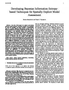
errors. We will expand the example in the following section to illustrate the development of the surrogate for a system without an analytical solution. For circular pipes with insulation and subject to external convective flow, the heat transfer involves two competing effects with relation to the thickness of the insulation material (Figure 4). With the addition of insulation, the conduction resistance increases, but the external convection resistance decreases due to the increase in external surface area. For small radius pipes (less than a critical radius=k/h, where k is the thermal conductivity of the insulation material and h is the external convective heat transfer coefficient), the heat transfer increases as the insulation thickness increases until it reaches a maximum when the outer radius (ro) of the insulation is equal to the critical radius. After the critical radius is reached, the heat transfer decreases as the insulation thickness increases (Figure 5). The heat transfer is linearly dependent on the convective heat transfer coefficient (h). To maximize the heat transfer of fluids through small diameter circular pipes, contrary to common sense, material is placed around the pipe. For this example, the design requirement is to select the insulation thickness for different convective conditions to maximize the heat transfer. This problem has an analytical solution shown in Equation 14, where Ti is the internal temperature of the fluid, T∞ is the external flow temperature, ri is the internal radius of the pipe, ro is the external radius of the insulation material and q is the heat transfer per length of pipe [16].

(13) k Ti

ro ri

Table 4. Measurements of percent error for twodimensional analytical functions.

CASE 1 CASE 2-1 CASE 2-2

st

1 stage 4th stage 1st stage 4th stage 1st stage 4th stage

f1 16.89 15.92 16.89 11.16 16.89 13.80

h, T∞

f2 15.98 22.27 15.98 5.90 15.98 8.63

Figure 4. Circular pipe with outside insulation in the presence of a convective flow.

q =

Ti − T∞ Ln ( r o / r i ) 1 + 2π k 2 π ro h

(14)

3.2. Surrogate model for a heat transfer system with an analytical solution The following example illustrates the development of a surrogate model using implicit bounds. The example uses a system with an analytical solution in order to compare the surrogate frameworks using accurate measurements of the

7

Copyright © 2001 by ASME

Design1

Design2

Design3

1 0.8 60

0.6 h

q

0.4

50 14 40

0.2

13

0

12 h

0.005 0.01

0

11

0.015 ro 0.02

The goal of surrogate modeling is to construct as accurate a model as possible with a small number of sampling points. The final surrogate model will describe the relationship between the heat transfer (q) and the following design parameters: radius of the insulation (ro) and convective heat transfer coefficient (h) over the range of values of interest to the designer. Twenty-five sampling points are distributed over the design space, using a maximin orthogonal array. In the first and second stages, ten points are sampled and five are sampled in the third stage (Figure 6). The following initial conditions are given: the internal temperature Ti is 423.15 K, the external flow temperature T∞ is 303.15 K, the thermal conductivity k is 0.15 W/mK, and the internal radius ri is 0.005 m. The ranges of interest for the two design parameters are ro [0.005 – 0.025 m] and h [10 – 14 W/m2K]. To illustrate the methodology, we construct two surrogate models: one using the constant variance framework and one using the covariance-based framework with implicit bounds. For the covariance-based framework, the implicit bounds are generated after the first stage. Table 5 compares the percent errors for the two approaches, showing that the model constructed using the covariance-based framework with implicit bounds yields smaller errors. The similarity between the surrogate model and the physical function for the heat transfer is illustrated in Figure 7.

Table 5. Percent error ep for surrogate and analytical solution. Covariance-based Constant Variance surrogate with implicit surrogate bounds 0.5670

0.5952

0.6

0.8

1

Figure 6. Sampling points for heat transfer system with an analytical solution.

Figure 5. Heat transfer (q) versus the external radius (ro) and the convective heat transfer coefficient (h).

0.5751

0.4

radius (ro) 0.025 10

1st stage 2nd stage 3rd stage

0.2

0.5751 0.5450 0.5431

q(t1,t2) 58

56

Analytical Function 3rd Stage Surrogate 54

0.2

0.4

0.6

0.8

1

t1=(ro-0.005)/0.025 t2=(h-10)/14=0.5

Figure 7. Heat transfer (q) and third stage surrogate model using implicit bounds.

4. DESIGN PROBLEM In the design of a wearable computer, a pipe, which contains a dielectric fluid, passes through a plastic structure that is used to increase the rigidity and provide mechanical support of the computer assembly. The design requirement is to maximize the heat transferred from the pipe, since the dielectric fluid is circulating in a closed-loop for cooling other components. The design variables include the length and height of the plastic support structure, depicted on Figure 8. The radius of circular pipe (ri) has been set at 0.005 m and the pipe must be in the center of the support structure. Both the height and the width are in the range of 0.015 to 0.05 m. Two of the walls are modeled as thermally insulated due to contact with the computer structure, which has a much lower thermal conductivity. The remaining two walls are subject to a convective airflow, at temperature T∞ = 303.15 K and with a convective heat transfer coefficient h = 10 W/m2K. The average temperature of the fluid entering the pipe is Ti = 423.15

8

Copyright © 2001 by ASME

K. This problem can be solved through numerical simulations of the governing energy equations using commercially available codes [17]. To construct the surrogate model, five simulations using a spectral element code are run for the first stage and five more are added in a second stage. Table 6 presents the values of both parameters in each simulation. The first and second stage surrogates are shown in Figures 9 and 10 as a function of non-dimensional length and height. While it would be possible

for the designer to perform multiple numerical simulations to determine the optimum, during the preliminary design stage, when the design is in flux, this effort is not warranted. Moreover, even though the surrogate requires effort to construct, once it has been constructed, it can continue to evolve with the design.

h,T∞ Insulated Wall

Insulated Wall

ri

50

Height

40 q 30

h,T∞

1 0.8 0.6 0.4Height 0.2

Length

20 Figure 8. Thermal design problem for a support structure that maximizes heat transfer. Table 6. Design parameters for each numerical simulation. st Length (m) Height (m) 1 stage 1 0.048 0.030 2 0.02 0.022 3 0.03 0.015 4 0.015 0.04 5 0.04 0.05 nd 2 stage Length (m) Height (m) 1 0.032 0.02 2 0.024 0.015 3 0.015 0.03 4 0.04 0.04 5 0.05 0.05

50 40 q 30 1 0.8 0.6 0.4Height 0.2

20 0 0.2

0.4 0.6 Length 0.8

10

Figure 9. Heat transfer (q) versus nondimensional length and height of the plastic support for first stage surrogate.

0 0.2

0.4 0.6 Length 0.8

10

Figure 10. Heat transfer (q) versus nondimensional length and height of plastic support for second stage surrogate.

5. CONCLUSIONS Using the covariance-based framework with implicit bounds to develop surrogate models enables designers to develop models of the interactions among design parameters even when they have little a priori knowledge about the response of the system. This multi-stage Bayesian approach results in surrogates that accurately model the system response. The ability to refine models and increase their accuracy in stages is valuable in the design process since it allows the models to evolve with the design. Thus, in the early design stages, approximate models that cover a large design space can be developed. As the design is refined, and new points in the design space are sampled, the scope of the model can be reduced and its accuracy increased without discarding the earlier information. Furthermore, the covariance-based framework using implicit bounds does not lose accuracy at points where data has been collected at previous stages. For the one-dimensional analytical function example in which the implicit bounds are used after the second stage, we obtain a 62% decrease in percent error. For the two-dimensional functions, an average decrease of 52% was found. The two parameters that describe the implicit bounds have the following effects: first, the previous stage surrogate influences the shape of the bounds that are created; second, the constant variance from the preceding stage influences the distance between the bounds. For the two-parameter heat transfer example with an

9

Copyright © 2001 by ASME

analytical solution, we obtain an error decrease of 9% after three stages of data collection. We are currently implementing the framework with an interface that will make it easy for designers to step through constructing and using a surrogate. ACKNOWLEDGMENTS This work has been supported by the National Science Foundation under grant DMI-9800565 and by DARPA through the program EDIFICE project HERECTIC N00014-99-0481. REFERENCES [1] Bukkapatnam, S., C-Y Lu, S., Ge, P., and Wang, N., 1999, “Backward Mapping Methodology for Design Synthesis,” Proceedings ASME Design Engineering Technical Conference DETC99/DTM-8766, Las Vegas, Nevada. [2] Osio, I. G., and Amon, C. H., 1996, “An Engineering Design Methodology with Multistage Bayesian Surrogates and optimal Sampling,” Research in Engineering Design, 68-2, pp. 189-206. [3] Krishnamurty, S., and Doraiswamy, S., 2000, “Bayesian Analysis in Engineering Model Assessment,” Proceedings ASME Design Engineering Technical Conferences and Computers and Information in Engineering Conference DETC2000/DTM-14546, Baltimore, MD [4] Shewry, M.C., and Wynn, H.P., 1987, “Maximum Entropy Sampling,” Journal of Applied Statistics, 14, pp. 165-170. [5] Leoni, N. J., 1999, “Integrating Information Sources into Global Models: A Surrogate Methodology for Product and Process Development,” Ph.D. Thesis, Carnegie Mellon University, Pittsburgh, PA. [6] Leoni, N., and Amon, C.H., 2000, “Bayesian Surrogates for Integrating Numerical, Analytical and Experimental Data” Application to Inverse Heat Transfer in Wearable Computers,” IEEE Transactions on Components and Packaging Technologies, 23, No. 1, pp. 23-32. [7] Sacks, J., Welch, W. J., Mitchell, T. J., and Wynn, H. P., 1989, “Design and Analysis of Computer Experiments,” Statistical Science, 4, No. 4, pp. 409-435. [8] Cressie, N., 1991, Statistics for Spatial Data, John Wiley and Sons. [9] Yesilyurt, S., Ghaddar, C., Cruz, M., and Patera, A. T., 1996, “Bayesian-Validated Surrogate for Noisy Computer Simulations; Application to Random Media,” SIAM Journal on Scientific Computing, 17, No. 4, pp. 973-992. [10] Otto, J. C., Paraschivoiu, M., Yesilyurt, S., and Patera, A. T., 1995, “Bayesian-Validated Computer Simulation Surrogates for Optimization and Design,” Proceedings ICASE Workshop on Multidisciplinary Design Optimization, Hampton, VA. [11] Osio, I. G., and Amon, C. H., in press, “Maximin Orthogonal Arrays for Large-Scale Computational Experiments,” Journal of Statistical Planning and Inference. [12] Hertz, J., Krogh, A., and Palmer, R., 1991, Introduction to the Theory of Neural Computation, Addison Wesley. [13] Box, G., and Draper, N. R., 1987, Empirical ModelBuilding and Response Surfaces, John Wiley & Sons.

[14] DeGroot, M. H., 1975, Probability and Statistics, AddisonWesley. [15] Mitchell, Y.J., and Morris, M.D., 1992, “Bayesian Design and Analysis of Computer Experiments: Two Examples,” Statistica Sinica, 2, pp. 359-379. [16] Incropera, F.P., and DeWitt, D.P., 1996, Fundamentals of Heat and Mass Transfer, John Wiley & Sons. [17] Jaluria, Y., 1987, Design and Optimization of Thermal Systems, McGraw-Hill. NOMENCLATURE Design matrix containing the sampling design D points v v v Covariance between the responses Y( t ) and K (t , s ) v Y( s ) v r v Vector of covariances between ( t ) and the k (t ) sampling points k Number of dimensions in the design space L (.)

Likelihood function

m

Number of sampling points

v t

V

k-vector of scalar design parameters

1/2

Standard deviations matrix

v

Y (t ) v

y (t ) r y p (D p )

v

(D p )

p −1

v θ v v ρ (t )

Scalar random variable Response to be modeled Vector of responses at sampling points of stage p Constant for a prior linear model Vector of predictions of prior at sampling points of stage p k-vector of correlation parameters

v

v σ( t )

Vector of correlations between ( t ) and the sampling points v Correlation between the responses Y( t ) and v Y( s ) v Standard deviation of Y( t )

Ω

Design space

Σ

Covariance matrix

v v ρ (t , s )

subscript

p

Stage of data collection

LB

Lower Bound

UB

Upper Bound

superscript

C.V.

Constant Variance

C.B.

Covariance-based

10

Copyright © 2001 by ASME