EARTHQUAKE ENGINEERING AND STRUCTURAL DYNAMICS Earthquake Engng Struct. Dyn. 2005; 00:1–22 Prepared using eqeauth.cls [Version: 2002/11/11 v1.00]
Developing efficient scalar and vector intensity measures for IDA capacity estimation by incorporating elastic spectral shape information‡ Dimitrios Vamvatsikos1,∗,† and C. Allin Cornell2 2
1 Department of Civil Engineering, National Technical University of Athens, Greece Department of Civil and Environmental Engineering, Stanford University, CA 94305-4020, U.S.A.
SUMMARY Scalar and vector Intensity Measures are developed for the efficient estimation of limit-state capacities through Incremental Dynamic Analysis (IDA) by exploiting the elastic spectral shape of individual records. IDA is a powerful analysis method that involves subjecting a structural model to several ground motion records, each scaled to multiple levels of intensity (measured by the Intensity Measure or IM ), thus producing curves of structural response parameterized by the IM on top of which limit-states can be defined and corresponding capacities can be calculated. When traditional IM s are used, such as the peak ground acceleration or the first-mode spectral acceleration, the IM -values of the capacities can display large record-to-record variability, forcing the use of many records to achieve reliable results. By using single optimal spectral values as well as vectors and scalar combinations of them on three multistory buildings significant dispersion reductions are realized. Furthermore, IDA is extended to vector IM s, resulting in intricate fractile IDA surfaces. The results reveal the most influential spectral regions/periods for each limit-state and building, illustrating the evolution of such periods as the seismic intensity and the structural response increase towards global collapse. The ordinates of the elastic spectrum and the spectral shape of each individual record are found to significantly influence the seismic performance and they c 2005 John Wiley & Sons, Ltd. are shown to provide promising candidates for highly efficient IM s. Copyright ° KEY WORDS : performance-based earthquake engineering; incremental dynamic analysis; capacity; intensity measure; limit-state; nonlinear
1. INTRODUCTION An important aspect of Performance-Based Earthquake Engineering (PBEE) is calculating, for a given building, capacities for the limit-states of interest and their corresponding mean annual frequencies of exceedance. A promising method that has been developed to meet these needs is Incremental Dynamic Analysis (IDA). It involves performing nonlinear dynamic analyses of the structural model under a
∗ Correspondence
to: Dimitrios Vamvatsikos, Theagenous 11, Athens 11634, Greece.
[email protected] ‡ Based on a short paper presented at the 13th World Conference on Earthquake Engineering, Vancouver, 2004 † E-mail:
Contract/grant sponsor: Sponsors of the Reliability of Marine Structures Affiliates Program of Stanford University
c 2005 John Wiley & Sons, Ltd. Copyright °
Received ? May 2004 Revised 9 March 2005 Accepted 11 March 2005
2
D. VAMVATSIKOS AND C. A. CORNELL
suite of ground motion records, each scaled to several intensity levels designed to force the structure all the way from elasticity to final global dynamic instability (Vamvatsikos and Cornell [1]). Thus, we can generate IDA curves of the structural response, as measured by an Engineering Demand Parameter (EDP , e.g., the maximum peak interstory drift ratio θmax ), versus the ground motion intensity level, measured by an Intensity Measure (IM , e.g., peak ground acceleration, PGA, or the 5%-damped first-mode spectral acceleration Sa (T1 , 5%)). Subsequently, limit-states (e.g., Immediate Occupancy or Collapse Prevention in FEMA [2]) can be defined on each IDA curve and the corresponding capacities can be calculated. The resulting capacities are then summarized, for example into appropriate fractiles, combined with probabilistic seismic hazard analysis results and integrated within a suitable PBEE framework to allow the calculation of the mean annual frequencies of exceeding each limit-state (Vamvatsikos and Cornell [3]). It is an unavoidable fact that the IDA curves and, correspondingly, the limit-state capacities display large record-to-record variability even for the simplest of structures, e.g., oscillators (Vamvatsikos and Cornell [4]). This observed dispersion is closely connected to the IM used; some IM s are more efficient than others, better capturing and explaining the differences from record to record, thus bringing the results from all records closer together. Compare, for example, Figures 1(a) and 1(b) where thirty IDA curves for a 9-story steel moment-resisting frame are plotted using PGA and Sa (T1 , 5%), respectively, as the IM . In both cases the variability from record to record is indeed remarkable, especially considering that the thirty records were chosen to represent a scenario earthquake and belong to a narrow magnitude and distance bin (Table I). However, PGA (Figure 1(a)) is proven to be deficient relative to Sa (T1 , 5%) (Figure 1(b)) in expressing the limit-state capacities of the 9-story; it increases the variability between the curves and, correspondingly, the dispersion of capacities everywhere on the IDAs. On the other hand, even the improvement achieved by Sa (T1 , 5%) still leaves something to be desired, as dispersions remain in the order of 40% – 50%. 3
6 5 4 3 2 1 0 0
0.05
0.1
maximum interstory drift ratio, θ max
(a) Thirty IDA curves versus PGA
0.15
"first−mode" spectral acceleration Sa(T1,5%) (g)
peak ground acceleration PGA (g)
7
2.5
2
1.5
1
0.5
0 0
0.05
0.1
0.15
maximum interstory drift ratio, θ max
(b) Thirty IDA curves versus Sa (T1 , 5%)
Figure 1. IDA curves for a T1 = 2.4 sec, 9-story steel moment-resisting frame with fracturing connections plotted against (a) PGA and (b) Sa (T1 , 5%).
Why should we search for such a better IM ? There is a clear computational advantage if we can select it a priori, before the IDA is performed. By reducing the variability in the IDA curves we need fewer records to achieve a given level of confidence in estimating the fractile IM -values of limit-state c 2005 John Wiley & Sons, Ltd. Copyright °
Earthquake Engng Struct. Dyn. 2005; 00:1–22
INTENSITY MEASURES WITH ELASTIC SPECTRAL SHAPE INFORMATION
3
capacities and the mean annual frequencies of limit-state exceedance. Typically, a reduction of the IM capacity dispersion by a factor of two means that we need four times fewer records to gain the same confidence in the fractile IM -capacity results (e.g., Vamvatsikos and Cornell [3]): We could get same quality results by using about eight instead of thirty records. Obviously, the computational savings would be enormous.
ln [Sa(τ,5%) / Sa(2.4s,5%)]
3
2
1
0
−1
−2 1
2
3
4
5
6
period, τ (s)
Figure 2. The 5%-damped elastic acceleration spectra for thirty scenario records, normalized to the first-mode period of the 9-story building.
Additionally, it is speculated that increasing the efficiency of the IM may also lead to improved sufficiency as well. A sufficient IM produces the same distribution of demands and capacities independently of the record selection, e.g., there is no bias in the fractile IM -capacities if we select records with low rather than high magnitudes or if the records do or do not contain directivity pulses (Luco [5]). The goals of efficiency and sufficiency are not necessarily tied together as the former aims at reducing the variability in the IDA results while the latter at reducing (or eliminating) their dependance on record characteristics other than the IM . Still, using a more efficient IM will bring the results from all records closer, and similarly bring close the IDA curves of records coming from different magnitudes or containing different directivity pulses, thus reducing the importance of any magnitude or directivity dependance. While Sa (T1 , 5%) is found to be both efficient and sufficient for first-mode-dominated, moderate period structures when directivity is not present (Shome and Cornell [6]), it is not necessarily so for other cases (Luco [5]). Therefore, it is important to try and improve our IM s beyond the capabilities of Sa (T1 , 5%). Figure 2 may provide some clues; therein we have plotted the 5%-damped acceleration spectra of the thirty records chosen to represent a scenario earthquake and appearing in Table I. The spectra have been normalized by Sa (2.4s, 5%), i.e., the value of Sa (T1 , 5%) at the first-mode period T1 = 2.4s of the 9-story building that we are using as an example. There is obviously much variability in the individual spectra that cannot be captured by just Sa (T1 , 5%). A structure is not always dominated by a single frequency and even then, when the structure sustains damage its properties change. Thus, spectral regions away from the elastic first-mode period, T1 , may become more influential. By taking the differences in the individual spectral shapes into account, we may be able to reduce the variability in the IDA curves and come up with an overall better IM . Such information may be incorporated into the IM by using appropriate inelastic spectral values c 2005 John Wiley & Sons, Ltd. Copyright °
Earthquake Engng Struct. Dyn. 2005; 00:1–22
4
D. VAMVATSIKOS AND C. A. CORNELL
Table I. The suite of thirty ground motion records used. No
Event
Station
φ◦
∗
Soil†
M‡
R§ (km)
PGA (g)
1 2 3 4 5 6 7 8 9 10 11 12 13 14 15 16 17 18 19 20 21 22 23 24 25 26 27 28 29 30
Loma Prieta, 1989 Northridge, 1994 Imperial Valley, 1979 Imperial Valley, 1979 Loma Prieta, 1989 San Fernando, 1971 Loma Prieta, 1989 Loma Prieta, 1989 Imperial Valley, 1979 Imperial Valley, 1979 Northridge, 1994 Loma Prieta, 1989 Loma Prieta, 1989 Imperial Valley, 1979 Imperial Valley, 1979 Imperial Valley, 1979 Loma Prieta, 1989 Loma Prieta, 1989 Superstition Hills, 1987 Imperial Valley, 1979 Imperial Valley, 1979 Imperial Valley, 1979 Loma Prieta, 1989 Loma Prieta, 1989 Superstition Hills, 1987 Imperial Valley, 1979 Imperial Valley, 1979 Loma Prieta, 1989 San Fernando, 1971 Loma Prieta, 1989
Agnews State Hospital LA, Baldwin Hills Compuertas Plaster City Hollister Diff. Array LA, Hollywood Stor. Lot Anderson Dam Downstrm Coyote Lake Dam Downstrm El Centro Array #12 Cucapah LA, Hollywood Storage FF Sunnyvale Colton Ave Anderson Dam Downstrm Chihuahua El Centro Array #13 Westmoreland Fire Station Hollister South & Pine Sunnyvale Colton Ave Wildlife Liquefaction Array Chihuahua El Centro Array #13 Westmoreland Fire Station Halls Valley WAHO Wildlife Liquefaction Array Compuertas Plaster City Hollister Diff. Array LA, Hollywood Stor. Lot WAHO
090 090 285 135 255 180 270 285 140 085 360 270 360 012 140 090 000 360 090 282 230 180 090 000 360 015 045 165 090 090
C,D B,B C,D C,D –,D C,D B,D B,D C,D C,D C,D C,D B,D C,D C,D C,D –,D C,D C,D C,D C,D C,D C,C -,D C,D C,D C,D –,D C,D –,D
6.9 6.7 6.5 6.5 6.9 6.6 6.9 6.9 6.5 6.5 6.7 6.9 6.9 6.5 6.5 6.5 6.9 6.9 6.7 6.5 6.5 6.5 6.9 6.9 6.7 6.5 6.5 6.9 6.6 6.9
28.2 31.3 32.6 31.7 25.8 21.2 21.4 22.3 18.2 23.6 25.5 28.8 21.4 28.7 21.9 15.1 28.8 28.8 24.4 28.7 21.9 15.1 31.6 16.9 24.4 32.6 31.7 25.8 21.2 16.9
0.159 0.239 0.147 0.057 0.279 0.174 0.244 0.179 0.143 0.309 0.358 0.207 0.24 0.27 0.117 0.074 0.371 0.209 0.18 0.254 0.139 0.11 0.103 0.37 0.2 0.186 0.042 0.269 0.21 0.638
∗
Component
†
USGS, Geomatrix soil class
‡
moment magnitude
§ closest
distance to fault rupture
(Luco [5]). This seems to be a promising method, as it directly incorporates the influence of the record on an oscillator that can yield and experience damage in a way similar to the structure. Still, in the context of PBEE, the use of inelastic spectral values requires new, custom-made attenuation relationships. On the other hand, using the elastic spectral values allows the use of the attenuation laws available in the literature. Therefore, there is still much to be gained from the use of IM s based on elastic spectra. Actually, studies by Shome and Cornell [6], Carballo and Cornell [7], Mehanny and Deierlein [8] and Cordova et al. [9] have shown that the elastic spectral shape can be a useful tool in determining an improved IM . Shome and Cornell [6] found that the inclusion of spectral values at the secondmode period (T2 ) and at the third-mode (T3 ), namely Sa (T2 , 5%) and Sa (T3 , 5%), significantly improved the efficiency of Sa (T1 , 5%) for tall buildings. Carballo and Cornell [7] observed greatly reduced variability in the EDP demands when spectral shape information was included by compatibilizing a suite of records to their median elastic spectrum. In addition, Mehanny and Deierlein [8] and Cordova et al. [9] observed an improvement in the efficiency of Sa (T1 , 5%) when an extra period, longer than c 2005 John Wiley & Sons, Ltd. Copyright °
Earthquake Engng Struct. Dyn. 2005; 00:1–22
INTENSITY MEASURES WITH ELASTIC SPECTRAL SHAPE INFORMATION
5
the first-mode was included by employing an IM of the form Sa (T1 , 5%)1−β Sa (c · T1 , 5%)β (with suggested values β = 0.5, c = 2). They also presented some evidence suggesting that sufficiency may be improved as well, since the new IM made the IDA curves of several near-fault records practically indistinguishable, regardless of the directivity-pulse period. Motivated by such encouraging results we are going to use the methodology and tools developed by Vamvatsikos and Cornell [1, 3] to better investigate the potential of incorporating elastic spectral shape information in IM s to reduce the dispersion in IDA results.
2. METHODOLOGY We will employ three different structures for our investigation into the potential use of the elastic acceleration spectrum. These will be a T1 = 1.8s 5-story steel chevron-braced frame and two steel moment-resisting frames designed for Los Angeles: a T1 = 2.4s 9-story with fracturing connections and a T1 = 4s 20-story with ductile connections. In all cases we used two-dimensional centerline models. The 5-story model includes ductile members and connections but realistically buckling braces (Bazzurro and Cornell [10]). The 9-story model incorporates ductile members, shear panels and realistically fracturing reduced beam section connections, while it includes the influence of interior gravity frames (Lee and Foutch [11]). The 20-story model (Luco and Cornell [12]) has ductile members and connections and it also accounts for the influence of the interior gravity frames. Finally, all models include a first-order treatment of global geometric nonlinearities (P-∆ effects). To perform IDA we used the suite of thirty records representing a scenario earthquake that was introduced earlier in Table I. These belong to a bin of relatively large magnitudes of 6.5 – 6.9 and moderate distances, all recorded on firm soil and bearing no marks of directivity. Each of these records was appropriately scaled to cover the entire range of structural response for each building, from elasticity, to yielding, and finally global dynamic instability. At each scaling level a nonlinear dynamic analysis was performed and a single scalar was used to describe the structural response, the Engineering Demand Parameter EDP according to current Pacific Earthquake Engineering Research (PEER) Center terminology (previously known as the Damage Measure DM , e.g., Vamvatsikos and Cornell [1]) . This will be θmax in our case. The scaling level and the associated ground motion intensity can be expressed by the selected IM , which will initially be Sa (T1 , 5%) for our investigation. By interpolating such pairs of Sa (T1 , 5%) and θmax values for each individual record we get thirty continuous IDA curves for each of the three buildings, shown as an example in Figure 1(b) for the 9-story. While usually only a handful of distinct limit-states of practical value would be defined on the IDA curves (e.g., Immediate Occupancy or Collapse Prevention in FEMA [2]), we will proceed to define a continuum of limit-states that completely cover the structural response: Each will be defined at a given θmax value to represent the capacity of the structure at a specific damaged state and level of response. Finally, the appropriate Sac (T1 , 5%)-values will be calculated, i.e., the values of Sa (T1 , 5%)-capacity for each record and each limit-state or value of θmax (Vamvatsikos and Cornell [1]). Our ultimate goal is to minimize the dispersion in the IM -values of capacities for each limit-state individually by selecting appropriate spectral values or vectors and functions of spectral values to be the IM . As a measure of the dispersion we will use the standard deviation of the logarithm of the IM -capacities, which is a natural choice for values that are approximately lognormally distributed (e.g., Shome and Cornell [6]). Fortunately, no further dynamic analyses are needed to change from Sa (T1 , 5%) to other IM s and perform this dispersion-minimization; all we need to do is to transform each limit-state’s Sac (T1 , 5%)values in the coordinates of the trial IM s and calculate their new dispersion. For example, if we want c 2005 John Wiley & Sons, Ltd. Copyright °
Earthquake Engng Struct. Dyn. 2005; 00:1–22
6
D. VAMVATSIKOS AND C. A. CORNELL
the dispersion of the capacities in PGA terms, then for each unscaled record (or at a scale factor of one) we know both the PGA and Sa (T1 , 5%)-values and the former can be appropriately scaled by the same factor that the value of Sac (T1 , 5%) implies; e.g., for the 9-story building, the unscaled record #5 (Table I) has Sa (T1 , 5%) = 0.114g and PGA = 0.279g, while global instability occurs at Sac (T1 , 5%) = 0.49g, representing a scale factor of 0.49/0.114 ≈ 4.3. Hence, the IM -capacity at the global instability limit-state in PGA terms is PGAc = 4.3 · 0.279 = 1.20g. Similarly we can accomplish such transformations for any IM based on elastic spectral values. Thus, we are taking full advantage of the observations in Vamvatsikos and Cornell [3], by appropriately postprocessing the existing dynamic runs instead of performing new ones. The adopted approach in evaluating the candidate IM s is very different from the one used by Shome and Cornell [6], Mehanny and Deierlein [8], Cordova et al. [9] and Luco [5]. There, the focus is on demands, i.e., EDP -values, all four studies looking for a single “broad-range” IM that will improve efficiency for all damage levels of a given structure. On the other hand, our search will be more focused, zeroing on each limit-state separately to develop a “narrow-range” IM that will better explain the given limit-state rather than all of them. Thus, we are able to follow the evolution of such IM s as damage increases in the structure, hopefully gaining valuable intuition in the process. Still, since we use only θmax to define the structural limit-states, our observations may or may not be applicable when limitstates are defined on other structural response measures (e.g., peak floor accelerations). The initial focus of our investigation will be on the efficiency gained by incorporating elastic spectrum information in the IM . We will start by investigating single spectral coordinates. This does not constitute an investigation of spectral shape per se as it focuses on the use of just one value at one period. Still, it will provide a useful basis as we expand our trial IM s to include vectors and scalar combinations of several spectral values. Another important issue will be the robustness offered by each IM , i.e., how much efficiency it retains when the user selects spectral values other than those chosen by the dispersion-minimization process. This is a key question when trying to identify a priori an appropriate IM in order to take advantage of its efficiency and use fewer records in the analysis. We are not aiming to provide the final answer for the best a priori IM , but rather to investigate the efficiency and the potential for practical implementation offered by several promising candidates.
3. USING A SINGLE SPECTRAL VALUE The use of a single spectral value, usually at the first-mode of the structure, i.e., Sa (T1 , 5%), has seen widespread use for IDAs, having being incorporated into the FEMA [2] guidelines and used throughout most of the current research. Obviously, it is an accurate measure for SDOF systems or first-mode-dominated structures in the elastic range. However, when higher modes are important or the structure deforms into the nonlinear range, it may not be optimal. There seems to be a consensus that when structures are damaged and move into the nonlinear region, period lengthening will occur (e.g., Cordova et al. [9]). In that sense, there may be some merit in looking for elastic spectral values at longer or, in general, different periods than the first-mode. Therefore we will conduct a search across all periods in the spectrum to determine the one that most reduces the variability in the IM -values of limit-state capacities. Some representative results are shown in Figure 3 for the 5-story building, for limit-states at four levels of θmax (Figure 4), namely 0.01% (elastic), 0.7% (early inelastic), 1% (highly nonlinear) and +∞ (global instability). The structure has obviously insignificant higher modes, since Sa (T1 , 5%) produces practically zero dispersion for the capacities in the elastic region (Figure 3, (a)-line). As the c 2005 John Wiley & Sons, Ltd. Copyright °
Earthquake Engng Struct. Dyn. 2005; 00:1–22
7
INTENSITY MEASURES WITH ELASTIC SPECTRAL SHAPE INFORMATION
"first−mode" spectral acceleration Sa(T1,5%) (g)
0.8
dispersion of IM capacities
0.7 0.6 0.5 0.4 0.3 (a) θmax = 0.0001
0.2
(b) θmax = 0.007 (c) θmax = 0.01
0.1
(d) θmax = inf
T1
0
1
2
3
4
5
6
5 (d)
4.5 4 3.5
16% IDA
3 2.5 (c)
2
50% IDA
(b) 1.5 1
(a)
84% IDA
0.5 0 0
0.01
period, τ (s)
Figure 3. Dispersion of the Sac (τ , 5%)-values versus period τ for four limit-states for the 5-story building.
0.03
0.04
5
0.7
dispersion of IM capacities
0.8
3
2 T1
0.5 0.4 0.3 0.2 PGA Sa(T1,5%) optimal Sa(τ,5%)
0.1
0.01
0.02
0.03
0.04
0.06
0.6
1
0 0
0.05
Figure 4. The fractile IDA curves and capacities for four limit-states (Figure 3) of the 5-story building.
6
4
period, τ (s)
0.02
maximum interstory drift ratio, θ max
0.05
0.06
maximum interstory drift ratio, θmax
Figure 5. The optimal period τ as it evolves with θmax for the 5-story building.
0 0
0.01
0.02
0.03
0.04
0.05
0.06
maximum interstory drift ratio, θ max
Figure 6. The dispersion for the optimal Sa (τ , 5%) compared to Sa (T1 , 5%) and PGA, versus the limitstate definition, θmax , for the 5-story building.
structure becomes progressively more damaged the optimal period τ moves away from T1 , lengthening to higher values as expected. Initially, only a narrow band of periods around the optimal τ display low dispersions. When close to global collapse (Figure 3, (d)-line), this band around the optimal period increases so that any period from 2s to 4s will achieve low dispersion, at worst 30% compared to about 40% when using Sa (T1 , 5%). A summary of the results is shown in Figure 5, where the optimal period is shown versus the θmax -value of all the limit-states considered, while the best achieved dispersion is presented in Figure 6, compared against the dispersion when using PGA and Sa (T1 , 5%). As observed earlier, the optimal period increases after yielding, from τ = T1 to τ = 2.4s. Similarly, the dispersion increases for all three IM s in Figure 6, but with the use of the optimal period the efficiency is improved at least by 40% compared to Sa (T1 , 5%). Similar results for the 9-story building are presented in Figure 7, for the limit-states appearing in Figure 8 at θmax equal to 0.5% (elastic), 5% (inelastic), 10% (close to global collapse) and +∞ (global c 2005 John Wiley & Sons, Ltd. Copyright °
Earthquake Engng Struct. Dyn. 2005; 00:1–22
8
"first−mode" spectral acceleration Sa(T1,5%) (g)
D. VAMVATSIKOS AND C. A. CORNELL
0.8
dispersion of IM capacities
0.7 0.6 0.5 0.4 0.3 (a) θmax = 0.005
0.2
(b) θmax = 0.05 (c) θmax = 0.1
0.1 T3
0
T2
(d) θmax = inf
T1
1
2
3
4
5
6
1.6 (d) 1.4
16%IDA
1 0.8
50%IDA
0.6
84%IDA
0.4 0.2 0 0
0.05
0.1
0.15
0.2
0.25
maximum interstory drift ratio, θ max
Figure 7. Dispersion of the Sac (τ , 5%) values versus period τ for four limit-states for the 9-story building.
Figure 8. The fractile IDA curves and capacities for four limit-states (Figure 7) of the 9-story building.
6
0.8 0.7
dispersion of IM capacities
5
4
period, τ (s)
(b)
1.2 (a)
period, τ (s)
3
2
(c)
T1
0.6 0.5 0.4 0.3 0.2 PGA Sa(T1,5%) optimal Sa(τ,5%)
1 0.1
T2 T3 0 0
0.05
0.1
0.15
0.2
maximum interstory drift ratio, θ max
Figure 9. The optimal period τ as it evolves with θmax for the 9-story building.
0 0
0.05
0.1
0.15
0.2
maximum interstory drift ratio, θ max
Figure 10. Dispersion for the optimal Sa (τ , 5%) compared to Sa (T1 , 5%) and PGA, versus the limitstate definition, θmax , for the 9-story building.
instability). The building has significant higher modes, as evident in Figure 7 [(a)-line], since the first mode is not optimal even in the elastic region. While all three modes, T1 , T2 and T3 , seem to locally produce some dispersion reduction, the overall best single period lies somewhere between the T1 and T2 , at τ ≈ 1.2s. As damage increases the optimal period lengthens to higher values, finally settling close to T1 when global instability occurs (Figure 7, (d)-line). In Figure 9, the results are summarized for all limit-states, showing the gradual lengthening of the optimal period. Similarly, in Figure 10 the optimal dispersion thus achieved is compared versus the performance of PGA and Sa (T1 , 5%). Remarkably, only in the elastic and near-elastic region does this single optimal spectral value provide some improvement over Sa (T1 , 5%), in the order of 10%; close to global collapse no gains are realized. For the 20-story structure the results for four limit-states are shown in Figure 11, for θmax equal to 0.5% (elastic), 2% (near-elastic), 10% (close to global collapse) and +∞ (global instability); each limitstate is shown versus the fractile IDAs in Figure 12. This is a building where higher modes are even c 2005 John Wiley & Sons, Ltd. Copyright °
Earthquake Engng Struct. Dyn. 2005; 00:1–22
9
0.8 T1
dispersion of IM capacities
0.7 0.6 0.5 0.4 0.3 (a) θmax = 0.005
0.2
(b) θmax = 0.02 (c) θmax = 0.1
0.1 T3
0
(d) θmax = inf
T2
1
2
3
4
5
6
"first−mode" spectral acceleration Sa(T1,5%) (g)
INTENSITY MEASURES WITH ELASTIC SPECTRAL SHAPE INFORMATION
0.7
(b) 0.4 50% IDA 0.3
84% IDA
0.2 0.1 0 0
0.05
0.1
0.15
0.2
Figure 12. The fractile IDA curves and capacities for four limit-states (Figure 11) of the 20-story building.
6
0.8 0.7
dispersion of IM capacities
5
period, τ (s)
(a)
maximum interstory drift ratio, θ max
Figure 11. Dispersion of the Sac (τ , 5%)-values versus period τ for four limit-states of the 20-story building.
T1
3
2
1
16% IDA
0.5
period, τ (s)
4
(d)
(c)
0.6
0.6 0.5 0.4 0.3 0.2
T2
0 0
PGA Sa(T1,5%) optimal Sa(τ,5%)
0.1
T3 0.05
0.1
0.15
0.2
maximum interstory drift ratio, θ max
Figure 13. The optimal period τ as it evolves with θmax for the 20-story building.
0 0
0.05
0.1
0.15
0.2
maximum interstory drift ratio, θ max
Figure 14. Dispersion for the optimal Sa (τ , 5%) compared to Sa (T1 , 5%) and PGA, versus the limitstate definition, θmax , for the 20-story building.
more important, and by looking at Figure 11 [(a)-line] it seems that, at least initially, the second-mode period T2 manages to explain more than T1 in the dispersion of the IM capacity values. The limit-states are defined on θmax , the maximum of the story drifts, which often appears in the upper stories at low ductilities and is thus quite sensitive to the higher frequencies. As damage increases the optimal period moves away from T2 and at global collapse reaches a value somewhere in the middle of T1 and T2 , at τ ≈ 2.5s. In Figure 13 the summarized results confirm the above observations for all limit-states. Similarly to the 9-story only small reductions in dispersion are realized with the use of one spectral coordinate (Figure 14). At least, in this case, using a single optimal period seems to achieve somewhat better performance than Sa (T1 , 5%) close to global collapse. Summarizing our observations, the use of a single optimal spectral value seems to offer some benefits, but mostly to structures with insignificant higher modes. For such structures it seems relatively easy to identify the optimal period, as it is invariably an appropriately lengthened value of the firstc 2005 John Wiley & Sons, Ltd. Copyright °
Earthquake Engng Struct. Dyn. 2005; 00:1–22
10
D. VAMVATSIKOS AND C. A. CORNELL
mode period T1 . One could almost say that practically any (reasonably) lengthened first-mode period will work well. On the other hand, when higher modes are present, one spectral value is probably not enough. There do exist specific periods that one can use to reduce the variability, but they appear in a very narrow range and are difficult to pinpoint as damage increases. It would be difficult to pick a priori a single period for such structures as a slight miss will probably penalize the dispersion considerably. Most probably, the reason behind this apparent difficulty is that even in the nonlinear range such structures are sensitive to more than one frequency. Thus, our attempt to capture this effect with just one period results in the selection of some arbitrary spectral coordinate that happens to provide the right “mix” of spectral values at the significant frequencies. Looking at all the previous figures it becomes obvious that missing by a little bit will again, in most cases, pump up the dispersion significantly. Obviously, this one period is not a viable solution for any but the structures dominated by the firstmode. On the other hand, the introduction of another spectral value, to form a vector or an appropriate scalar combination of two periods, might prove better.
4. USING A VECTOR OF TWO SPECTRAL VALUES The use of more than one discrete spectral value necessitates the development of a framework for the use of vector IM s. While the definitions set forth in Vamvatsikos and Cornell [1] do provide for a vector IM , up to now no formal framework has been developed on how to postprocess and summarize such IDAs. So, before we proceed with our spectral shape investigation, we will propose a methodology to deal with vector IM s. 4.1. Postprocessing IDAs with vector IMs The most important thing that we must keep in mind is that the IDA per se remains unchanged and no need exists to rerun the results that we have acquired; this is all about postprocessing, as explained in Vamvatsikos and Cornell [3]. On the other hand, there are some conceptual differences between a scalar and a vector of IM s. Since the IM must in both cases represent the scaling of the ground motion record, the scalar IM has to be scalable, i.e., be a function of the scale factor of the record (Vamvatsikos and Cornell [1]). However, for a vector of IM s it would be redundant and often confusing if more than one of the elements were scalable. Hence, we will focus on vectors where only one of the elements can be scaled, while the others are scaling-independent. That is not to say, for example, that when we have Sa (T1 , 5%) in a vector, other spectral values are not acceptable. Rather, we will replace such extra spectral values by their ratio over Sa (T1 , 5%) (and similarly normalize any other scalable IM ); thus, we convey only the additional information that the new elements in the vector bring in with respect to our primary scalable (scalar) IM . In this case it is quite precise to speak of this additional information (one or more additional spectral ratios) as reflecting the influence of spectral shape (rather than the amplitude of the record). Following a similar procedure as for a single scalable IM , we will use splines to interpolate the discrete IDA runs for each record versus the scalable IM from the vector (Vamvatsikos and Cornell [1]). Then, we can plot the IDA curves for all records versus the elements of the vector, as in Figure 15 for the 5-story braced frame and a vector of Sa (T1 , 5%) (scalable) and the spectral ratio Rsa (1.5, T1 ) = Sa (1.5T1 , 5%)/Sa (T1 , 5%) (non-scalable). Contrary to the usual practice of plotting the IM on the vertical axis, we will now plot both IM s on the two horizontal axes and put the EDP on the vertical one, to visually separate the “input” from the “output”. As a consequence the flatlines are now c 2005 John Wiley & Sons, Ltd. Copyright °
Earthquake Engng Struct. Dyn. 2005; 00:1–22
11
0.03 0.02 0.01 0 2 1.5 1
Sa(1.5T1,5%)
0.5
Sa(T1,5%)
0
0
1
0.5
1.5
2
2.5
Sa(1.5T1,5%) / Sa(T1,5%)
1.6
0.025
1.4 0.02
1.2 0.015
1 0.8
0.01
0.6 0.005
0.4 0.5
1
1.5
2
2.5
Sa(T1,5%) (g)
Figure 17. The median contours for thirty IDA curves for the 5-story building in Sa (T1 , 5%) and Rsa (1.5, T1 ) coordinates. Their color indicates the level of θmax as shown in the color bar.
0.03 0.02 0.01 0 2 1.5 1 0.5 0
0
1
0.5
1.5
2
2.5
Sa(T1,5%) (g)
Figure 16. The median IDA surface for the 5-story building in Sa (T1 , 5%) and Rsa (1.5, T1 ) coordinates. 1.8
0.03
1.8
0.04
Sa(1.5T1,5%) Sa(T1,5%)
Sa(T1,5%) (g)
Figure 15. The thirty IDA curves for the 5-story building in Sa (T1 , 5%) and Rsa (1.5, T1 ) coordinates.
0
maximum interstory drift ratio, θ max
0.04
Sa(1.5T1,5%) / Sa(T1,5%)
maximum interstory drift ratio, θ max
INTENSITY MEASURES WITH ELASTIC SPECTRAL SHAPE INFORMATION
1.6 1.4 1.2 1 50% IM|EDP
0.8
84% IM|EDP
0.6 0.4 0
16% IM|EDP
0.5
1
1.5
2
2.5
Sa(T1,5%) (g)
Figure 18. The 16%, 50% and 84% capacity lines at the limit-state of θmax = 0.016 for the 5-story building.
vertical lines, rather than horizontal ones. Still, we are able to interpolate only along the scalable IM , while for the non-scalable one we are left with separate, discrete curves. We need to take an extra step here and make the results continuous in the other IM as well, which is why we will introduce summarization at this point. However, we are not able to use cross-sectional fractiles, as we did for single IM s in Vamvatsikos and Cornell [3]. That would require several values of EDP at each level of the non-scalable IM , practically impossible with a limited number of records. We can use instead the symmetric-neighborhood running fractiles (Hastie and Tibshirani [13]) with a given window length to achieve the same purpose. The optimal window length can be chosen, e.g., through cross-validation (Efron and Tibshirani [14]), or by adopting a reasonable fraction of the sample size. In our case, we selected 30% of the sample size, i.e., used the 0.3 × 30 = 9 symmetrically closest records to approximate the fractile value for each level of the non-scalable IM . The resulting median IDA surface appears in Figure 16. Now is the time to define limit-state capacities. It can be easily done using EDP -based rules for all limit-states, with θmax = +∞ resulting in the flatlines for global instability. Imagine horizontal planes, c 2005 John Wiley & Sons, Ltd. Copyright °
Earthquake Engng Struct. Dyn. 2005; 00:1–22
12
D. VAMVATSIKOS AND C. A. CORNELL
each for a given EDP -value, cutting the IDA surface. The results can be easily visualized as contours of the fractile IDA surface, seen in Figure 17 for the median. Obviously, now the median capacity for a given limit-state is not a single point, as for scalar IM s, rather a whole line, as the ones appearing in Figure 17. As an example, we are showing in Figure 18 the 16%, 50% and 84% capacity lines for a limit-state at θmax = 1.6%, close to the onset of global instability. These correspond to our best estimate of the 16%, 50% and 84% vector IM -value of the limit-state capacity. For example, if several records had Rsa (1.5, T1 ) = 1.2, then if scaled to Sa (T1 , 5%) ≈ 0.5g (to reach the 16% capacity line) only 16% of them would cause the structure to violate the limit-state, and they would have to be scaled to only Sa (T1 , 5%) ≈ 0.6g for 84% of them to cause limit-state exceedance. On the other hand, if another set of records were comparatively less rich in the longer periods, e.g., if Rsa (1.5, T1 ) = 0.5, they would have to be scaled to Sa (T1 , 5%) ≈ 1g to cause 50% of the records to violate this same limit-state. In retrospect, notice that we have slightly altered the “standard” IDA post-processing, as defined by Vamvatsikos and Cornell [1, 3]. For scalar IM s we would first define limit-states points on each IDA and then summarize, while for vector IM s it is advantageous to reverse these steps. Keep in mind though that if we are using only EDP -based rules for the definition of limit-states, as we do here, then we can similarly reverse these steps for the scalar IM . The results will be exactly the same, as explained in Vamvatsikos and Cornell [3]: The (100 − x)%-fractile IDA limit-state capacities for Immediate Occupancy and Global Instability (and all other EDP -based limit-states) reside on the x%fractile IDAs. On the other hand, this is not the case for the FEMA-350 [2] definition of the Collapse Prevention limit-state. It is partially based on the change of the slope of the IDA (Vamvatsikos and Cornell [1]), therefore it is clearly not a simple EDP -based limit-state. As a final note, it is important to observe how we were forced to introduce summarization over windows rather than stripes. By introducing an extra IM , we may have explained some of the variability in the capacities but we have also increased the dimensionality of the sample space, thus the data is more sparse. Where we used to have 30 points for each level (stripe) of the scalable IM , we now have only a few points for whole regions of the unscalable IM . Obviously, we cannot keep introducing extra dimensions, otherwise we will be facing extreme lack-of-data problems. 4.2. Investigating the vector of two spectral values Clearly, for the 5-story building with negligible higher modes, using a vector instead of a scalar IM produces very impressive results. The introduction of Rsa (1.5, T1 ) provides significant insight into the seismic behavior of the 5-story, as seen in Figure 17; for records with Rsa (1.5, T1 ) > 1, as its period lengthens the damaged structure falls in a more aggressive part of the spectrum and is forced to fail at earlier Sa (T1 , 5%) levels, exhibiting IDAs with rapid softening. On the other hand, if Rsa (1.5, T1 ) < 1 the period lengthening helps to relieve the structure allowing the IDA to harden and reach higher flatlines in terms of Sa (T1 , 5%). Actually, the less aggressive the record is at longer periods (lower Rsa (1.5, T1 )) the more the IDA hardens. The introduction of the extra IM has helped explain some of the record-to-record variability in the Sa (T1 , 5%) capacities for almost any level of EDP , i.e., for any limit-state. Additional studies show that such results are not very sensitive to the spectral ratio that we choose to use. At least for the 5-story building almost any such lengthened period will provide some explanation of the variability in capacity. On the other hand though, it may not be so for other buildings. As shown for the 9-story and 20-story buildings in Figures 19 and 20 respectively, using a vector of Sa (T1 , 5%) and Rsa (1.5, T1 ) yields little or no additional information compared to just Sa (T1 , 5%). These buildings have significant higher-mode influence, hence we have to use a spectral coordinate at a period lower c 2005 John Wiley & Sons, Ltd. Copyright °
Earthquake Engng Struct. Dyn. 2005; 00:1–22
13
INTENSITY MEASURES WITH ELASTIC SPECTRAL SHAPE INFORMATION
1 1.2
0.12
0.18
0.9 0.16 0.1
Sa(1.5T1,5%) / Sa(T1,5%)
Sa(1.5T1,5%) / Sa(T1,5%)
1.1 1 0.9
0.08
0.8 0.06
0.7 0.6
0.04
0.8 0.14
0.7
0.12
0.6
0.1
0.5
0.08
0.4
0.06
0.5
0.3 0
0.04
0.3
0.02
0.4
0.02
0.5
1
0.2 0
1.5
0.1
0.2
0.3
0.4
0.5
0.6
Sa(T1,5%) (g)
Sa(T1,5%) (g)
Figure 19. Median contours colored by θmax for the 9-story building in Sa (T1 , 5%) and Rsa (1.5, T1 ) coordinates. We see little improvement over Sa (T1 , 5%).
Figure 20. Median contours colored by θmax for the 20-story building in Sa (T1 , 5%) and Rsa (1.5, T1 ) coordinates. The use of a vector has small influence.
5.5 0.2
5
Sa(0.5T1,5%) / Sa(T1,5%)
0.18
4.5 0.16
4
0.14
3.5
0.12
3
0.1
2.5
0.08
2
0.06
1.5
0.04 0.02
1 0
0.1
0.2
0.3
0.4
0.5
0.6
Sa(T1,5%) (g)
Figure 21. Median contours colored by θmax for the 20-story building in Sa (T1 , 5%) and Rsa (0.5, T1 ) coordinates. Some variability is explained but the contours are not simple. 22
3
2.5
0.12 0.1
2 0.08 0.06
1.5
0.04
1 0.02
0.12
20
Sa(0.3T1,5%) / Sa(T1,5%)
Sa(0.7T1,5%) / Sa(T1,5%)
0.14
0.1
18 16
0.08
14 12
0.06
10 8
0.04
6 4
0.02
2 0
0.5
1
1.5
0
0.1
0.2
0.3
0.4
0.5
0.6
Sa(T1,5%) (g)
Sa(T1,5%) (g)
Figure 22. Median contours colored by θmax for the 9-story building in Sa (T1 , 5%) and Rsa (0.7, T1 ) coordinates. The contours have power-law shape.
Figure 23. Median contours colored by θmax for the 20-story building in Sa (T1 , 5%) and Rsa (0.3, T1 ) coordinates. The contours have power-law shape.
c 2005 John Wiley & Sons, Ltd. Copyright °
Earthquake Engng Struct. Dyn. 2005; 00:1–22
14
D. VAMVATSIKOS AND C. A. CORNELL
than T1 to gain resolution. Still the shape of the contours may no longer be the simple, monotonic, almost power-law shape that was observed for the 5-story. This happens, for example, in Figure 21 for the 20-story when Rsa (0.5, T1 ) is used in addition to Sa (T1 , 5%) (where 0.5T1 ≈ 1.5T2 for this building): the most aggressive records are the ones with Rsa (0.5, T1 ) ≈ 2, while lower or higher values of the spectral ratio will both indicate more benign records. Still, even for these complex buildings, there exist periods that explain well the variability and even show the familiar, power-law shape of the contours, as shown for the 9-story when we use Rsa (0.7, T1 ) (where 0.7T1 ≈ 2T2 for the 9-story) in Figure 22, and even the 20-story when we introduce Rsa (0.3, T1 ) in Figure 23 (where 0.3T1 ≈ T2 for the 20-story). Clearly, there is great potential in using a vector of two spectral values, but the question remains whether the appropriate periods for its use are easy to determine, especially a priori.
5. USING A POWER-LAW FORM WITH TWO OR THREE SPECTRAL VALUES By observing the power-law shape of the contours in Figures 17, 22 and 23 it becomes obvious that they can be approximated for each of the three buildings by the equation Sac (T1 , 5%) ≈ α Rsa (1.5, T1 )−β
(1)
where α , β are the fitted coefficients. Even though for a given building the β -value is not constant for all limit-states, as the contours have higher curvature for higher EDP -values, we can still specify some reasonable β -value that will be adequate for most of them. In that case, we can rewrite Equation (1) as
α ≈ Sac (T1 , 5%) Rsa (1.5, T1 )β
(2)
and interpret it as follows: by multiplying Sac (T1 , 5%) capacity values by Rsa (1.5, T1 )β , we can bring them closer, almost to an (arbitrary) constant. In other words, Sa (T1 , 5%)Rsa (1.5, T1 )β is a scalar IM that will retain much of the vector IM ’s ability to reduce dispersion in limit-state capacities. How much reduction it will achieve will depend on our ability to select a proper β -value and the goodness-of-fit of Equation (1) to the contour. Not surprisingly, it is such a form that Shome and Cornell [6], Mehanny and Deierlein [8] and Cordova et al. [9] have used to create a new, more effective scalar IM . While the idea there was mostly driven by the need to be able to use existing attenuation laws to create hazard curves for the new IM (Cordova et al. [9]), they have come very close to an accurate approximation of the contour shape. Motivated by the above results we intend to perform a search for the optimally efficient IM of the form
IM ≡ Sa (τa , 5%)1−β Sa (τb , 5%)β · ¸ Sa (τb , 5%) β = Sa (τa , 5%) Sa (τa , 5%)
(3)
where τa and τb are arbitrary periods and β ∈ [0, 1]. Notice the difference with Shome and Cornell [6] who constrain both periods to be T1 and T2 respectively, or Mehanny and Deierlein [8] and Cordova et al. [9], who chose to constrain one of the periods to be T1 . Instead, we intend to let the optimization find the best values, τa , τb and β . Additionally, we will investigate a power-law form containing three spectral values or, equivalently, c 2005 John Wiley & Sons, Ltd. Copyright °
Earthquake Engng Struct. Dyn. 2005; 00:1–22
INTENSITY MEASURES WITH ELASTIC SPECTRAL SHAPE INFORMATION
15
a single spectral value and two spectral ratios:
IM ≡ Sa (τa , 5%)1−β −γ Sa (τb , 5%)β Sa (τc , 5%)γ · ¸ · ¸ Sa (τb , 5%) β Sa (τc , 5%) γ = Sa (τa , 5%) (4) Sa (τa , 5%) Sa (τa , 5%) where τa , τb and τc are arbitrary periods, β , γ ∈ [0, 1] and β + γ ≤ 1. The optimal two periods for the 5-story building appear in Figure 24 over a range of limit-states from elasticity to global collapse. At elasticity, the two periods converge to the first mode, T1 , since the structure has practically no higher mode effects. As damage increases one of the periods hovers close to T1 while the other increases and fluctuates about 50% higher. The optimal value of β is always about 0.5, favoring equal weighting of the two periods. Comparing Figures 6 and 26 it becomes obvious that the use of two spectral values reduces the capacity dispersion by a small amount relative to the use of a single optimal value. While Sa (T1 , 5%) would achieve about 40% dispersion and a single optimal period would reduce this to 25%, the use of two periods only brings it down to 20%. If we introduce a third spectral value for the 5-story through Equation 4, then we come up with the three optimal periods shown in Figure 25 for a range of limit-states. Again, in elasticity, the three periods start at T1 and then they slowly separate. One period stays at about T1 and the rest gradually increase. When close to global collapse the second one is 50% higher and the third 100% higher than T1 . Again, equal weighting seems to be the rule for all limit-states since the optimal values are β ≈ γ ≈ 1/3. The dispersion reduction is even less spectacular than before (Figure 26), reaching a level of just 18% at global collapse compared to the 20% of the two spectral values. Clearly, we have reached the limits of what the elastic spectral shape can do for this building. As expected, when higher modes are insignificant, one, maybe two, periods will be enough to determine an improved, near-optimal IM , cutting down dispersion by a factor of two relative to Sa (T1 , 5%). Adding more complexity to the IM does not seem to help efficiency, as the system is not that complex itself. When practically implementing such IM s before the dynamic analyses are performed, it is important that efficiency remains high even when not using the (unknown a priori) optimal periods. To investigate the sensitivity of the proposed scalar IM s we have simulated random user choices for the period(s) used for the single spectral value or the power-law combinations of two or three values. The user is supposed to have picked periods uniformly distributed within ±20% of the optimal values for each IM and to have selected equal weighting of spectral values in the power-law (i.e., β = 1/2 or β = γ = 1/3). Such simulations are repeated numerous times for each limit-state (i.e., value of θmax ) and the achieved suboptimal dispersions are calculated for each IM . In Figure 27 we are plotting the 84%-fractile of the resulting sample of suboptimal dispersions for the single period and the two power-law combinations versus the θmax definition of each limit-state; i.e., we are focusing on a worse-than-average scenario. For comparison, the dispersion when using Sa (T1 , 5%) and when using the optimal three periods powerlaw is also shown. Obviously, the largest effect for the 5-story is in the elastic region, where not using T1 is a very bad choice in all cases. In the nonlinear range, missing the optimal period seriously degrades the performance of a single IM , bringing its dispersion to about 30%, a fact also observed in Figure 3. On the other hand, the two and three period combinations perform relatively well, managing to keep a dispersion of about 25% and 20%. Again, just as when using a vector of two spectral values, the power-law form is quite stable, even more so than using a single spectral value, since relatively large changes away from the optimal periods do not influence significantly the dispersion reduction of the power-law IM . Practically, in the post-yield region, using the first mode plus e.g., a 50% increased period, with β = 0.5 (i.e., equal weight on both spectral values) will in general produce good results. Actually these conclusions are quite in agreement with Cordova et al. [9]. c 2005 John Wiley & Sons, Ltd. Copyright °
Earthquake Engng Struct. Dyn. 2005; 00:1–22
D. VAMVATSIKOS AND C. A. CORNELL
6
6
5
5
4
4
period, τ (s)
period, τ (s)
16
3
2
3
2
T1
T1
1
1
0 0
0.01
0.02
0.03
0.04
0.05
0 0
0.06
maximum interstory drift ratio, θ max
0.03
0.04
0.05
0.06
Figure 25. The three optimal periods τa , τb , τc as they evolve with θmax for the 5-story building. 0.8
0.8 PGA Sa(T1,5%) 1 best period 2 best periods 3 best periods
0.6
Sa(T1,5%) 1 period 2 periods 3 periods 3 best periods
0.7
0.5 0.4 0.3 0.2
dispersion of IM capacities
0.7
dispersion of IM capacities
0.02
maximum interstory drift ratio, θ max
Figure 24. The two optimal periods τa , τb as they evolve with θmax for the 5-story building.
0.6 0.5 0.4 0.3 0.2 0.1
0.1 0 0
0.01
0.01
0.02
0.03
0.04
0.05
0.06
maximum interstory drift ratio, θ max
Figure 26. The dispersions for the 5-story building for PGA and Sa (T1 , 5%) versus the optimal one, two and three periods scalar IM s.
0 0
0.01
0.02
0.03
0.04
0.05
0.06
maximum interstory drift ratio, θ max
Figure 27. The 84% fractile of the suboptimal dispersion for a single period and power-law forms of two or three periods for the 5-story building, shown versus the dispersion achieved by Sa (T1 , 5%) and the optimal three-periods power-law IM .
In the case of the 9-story building the two optimal periods appear in Figure 28 and the three best in Figure 29. In the first case, the smaller period seems to stay at T2 while the higher one starts from T1 and increases to some higher value, only to return back to T1 again. For the three periods, the results seem to favor one period at T1 , another at T2 and a third at about twice T1 . Similarly to the 5-story, equal weighting is the optimal strategy for both IM s and almost all limit-states. With either two or three periods, as seen in Figure 30, the dispersion reduction is about the same. Actually, the dispersion drops from 40% for one optimal period (or even for just Sa (T1 , 5%)), to less than 25–30% when two or more periods are used. Again, it seems that two spectral values are enough for this first-mode-dominated building and clearly better than just one. What is of more value though is that the efficiency of the two or three-element IM is very stable relative to the choices of the periods and the β , γ weights. In Figure 31 we plot the results of the c 2005 John Wiley & Sons, Ltd. Copyright °
Earthquake Engng Struct. Dyn. 2005; 00:1–22
17
6
6
5
5
4
4
period, τ (s)
period, τ (s)
INTENSITY MEASURES WITH ELASTIC SPECTRAL SHAPE INFORMATION
3
2
T1
3
2
1
T1
1 T2 T3
0 0
T2 T3 0.05
0.1
0.15
0 0
0.2
Figure 28. The two optimal periods τa , τb as they evolve with θmax for the 9-story building.
0.15
0.2
0.8 PGA Sa(T1,5%)
0.7
1 best period 2 best periods 3 best periods
0.6
Sa(T1,5%) 1 period 2 periods 3 periods 3 best periods
0.7
dispersion of IM capacities
dispersion of IM capacities
0.1
Figure 29. The three optimal periods τa , τb , τc as they evolve with θmax for the 9-story building.
0.8
0.5 0.4 0.3 0.2
0.6 0.5 0.4 0.3 0.2 0.1
0.1 0 0
0.05
maximum interstory drift ratio, θ max
maximum interstory drift ratio, θmax
0.05
0.1
0.15
0.2
maximum interstory drift ratio, θmax
Figure 30. The dispersions for the 9-story building for PGA and Sa (T1 , 5%) versus the optimal one, two and three periods scalar IM s.
0 0
0.05
0.1
0.15
0.2
maximum interstory drift ratio, θ max
Figure 31. The 84% fractile of the suboptimal dispersion for a single period and power-law forms of two or three periods for the 9-story building, shown versus the dispersion achieved by Sa (T1 , 5%) and the optimal three-periods power-law IM .
previously described sensitivity analysis for the 9-story. Clearly, using only one (suboptimal) period is often worse or at most as good as when using Sa (T1 , 5%), as observed in Figure 7 as well. On the other hand, with two or three periods, equally weighted in a power-law form, the IM is considerably more robust and relatively reasonable efficiency is maintained. If we follow our observations and set one value around T1 , another at about T2 and maybe a third 50% or 100% higher than T1 , then weigh them equally (β = 1/2 or β = γ = 1/3), a dispersion of about 30% is easily achieved in contrast to the elusive single optimal period. Figure 32 shows the best two periods for the 20-story building. One seems to stay somewhere in the middle of T2 and T3 while the other is a lengthened version of the first mode, perhaps by 30–50%. The picture is clearer for the three best periods in Figure 33, where each seems to be a (roughly) 50% lengthened version of one of the three elastic modes, T1 , T2 and T3 . The optimal weights are roughly c 2005 John Wiley & Sons, Ltd. Copyright °
Earthquake Engng Struct. Dyn. 2005; 00:1–22
18
D. VAMVATSIKOS AND C. A. CORNELL
6
6
5
5
4
T1
period, τ (s)
period, τ (s)
4
3
T1
3
2
2
T2
T2
1
1 T3 0 0
T3 0.05
0.1
0.15
0 0
0.2
Figure 32. The two optimal periods τa , τb as they evolve with θmax for the 20-story building.
0.15
0.2
0.8 PGA Sa(T1,5%)
0.7
1 best period 2 best periods 3 best periods
0.6
Sa(T1,5%) 1 period 2 periods 3 periods 3 best periods
0.7
dispersion of IM capacities
dispersion of IM capacities
0.1
Figure 33. The three optimal periods τa , τb , τc as they evolve with θmax for the 20-story building.
0.8
0.5 0.4 0.3 0.2
0.6 0.5 0.4 0.3 0.2 0.1
0.1 0 0
0.05
maximum interstory drift ratio, θ max
maximum interstory drift ratio, θ max
0.05
0.1
0.15
0.2
maximum interstory drift ratio, θmax
Figure 34. The dispersions for the 20-story building for PGA and Sa (T1 , 5%) versus the optimal one, two and three periods scalar IM s.
0 0
0.05
0.1
0.15
0.2
maximum interstory drift ratio, θ max
Figure 35. The 84% fractile of the suboptimal dispersion for a single period and power-law forms of two or three periods for the 20-story building, shown versus the dispersion achieved by Sa (T1 , 5%) and the optimal three-periods power-law IM .
equal for all two or three periods. The dispersion reduction is significant in both cases, reaching down to 25% versus the 35% achieved by a single optimal period or the 40% of Sa (T1 , 5%) (Figure 34). While the use of three periods rather than two seems to offer little benefit, actually it makes the IM quite easier to define. Additionally the results of the sensitivity analysis in Figure 35 suggest that efficiency remains relatively high when three suboptimal periods are employed, versus two or one. Simply by increasing all three elastic periods by some reasonable percentage and employing equal weights (β = γ = 1/3) works fine for all limit-states, achieving dispersions in the order of 30%. In conclusion, it seems that the use of the power-law form with two or three spectral values helps even when the higher modes are significant. Actually, the more significant they are, the more periods we might want to include. The benefit is not so much in the reduction of dispersion, rather in the robustness of the IM and the ability to identify it a priori. The sensitivity of the power law IM s to suboptimal c 2005 John Wiley & Sons, Ltd. Copyright °
Earthquake Engng Struct. Dyn. 2005; 00:1–22
INTENSITY MEASURES WITH ELASTIC SPECTRAL SHAPE INFORMATION
19
user choices significantly decreases when more spectral values are included. Thus, it is not necessary to propose a “magic set” of parameters for each structure: In the inelastic range any reasonably chosen number of equally weighted periods that lie somewhat higher than the elastic ones will provide good dispersion reduction for most cases. Further investigation of more structures is needed before some concrete proposals are made, but the concept looks promising.
6. USING ALL SPECTRAL VALUES The problems encountered with all previous attempts to use the spectral shape mainly stem from the fact that we were looking for distinct “perfect” periods. This in part made the problem quite more difficult, as we were trying to describe the full spectral shape with only one or two spectral ratios. Using more spectral shape information will hopefully open up some easier paths. Still, visualizing an IM vector with more than one spectral ratio would be hard and it would be equally difficult to create enough data to fill the extra dimensions. On the other hand, the collapsed power-law form of the vector to a scalar suggests an easier way to approach this problem. Including more spectral coordinates in Equation (1) is relatively straightforward, while finding the right weight coefficients may be handled by standard linear regression methods, penalized to reflect the sample size limitations. Taking one step further, there exist methods in statistics that can treat each record’s spectrum as a single, functional predictor, thus taking into consideration the shape of the full spectrum and use it as a predictor for limit-state capacity. In formal terms we are proposing the use of a functional linear model (Ramsay and Silverman [15]) that will use each record’s spectrum to predict a scalar response, i.e., its limit-state Sac,i (T1 , 5%)-capacity derived from the IDA curve of that i-th record. In essence, we are proposing the use of the linear functional model · ¸ Z te Sa (τ , 5%) ln Sac,i (T1 , 5%) = α + β (τ ) ln (5) dτ + εi Sa (T1 , 5%) ts where α is the regression intercept, β (τ ) is the regression coefficient function, ts and te are the starting and ending periods that bound the spectral region of interest and, finally, εi are the independent and normally distributed errors (with a mean of zero). This can be thought as a conventional multivariate linear regression model, only we can have an infinite number of predictors, or degrees of freedom, in our fitting. Of course, having infinite parameters and only a finite number of responses allows such a model to actually interpolate the responses, if we choose so. This would not provide a meaningful estimator, but can be remedied by sufficiently smoothing the coefficient function β (τ ) at a level easily found through cross-validation. We end up with a model to predict limit-state capacities that can be easily imagined to be of the same power-law form as the one we have introduced to collapse the vector of two IM s into a scalar in Equation (1). If we use a trapezoidal rule to perform the integration, then we can write Equation (5) as: ¸ · n Sa (τi , 5%) ln Sac,i (T1 , 5%) ≈ α + ∑ β (τi ) ln ∆τ ⇔ Sa (T1 , 5%) j=1 ¸ n · Sa (τi , 5%) β (τi )∆τ c,i α Sa (T1 , 5%) ≈ e ∏ ⇔ j=1 Sa (T1 , 5%) ¸ n · Sa (τi , 5%) −β (τi )∆τ eα ≈ Sac,i (T1 , 5%) ∏ (6) j=1 Sa (T1 , 5%) c 2005 John Wiley & Sons, Ltd. Copyright °
Earthquake Engng Struct. Dyn. 2005; 00:1–22
20
D. VAMVATSIKOS AND C. A. CORNELL
−0.16
regression coefficient
−0.18
−0.2
−0.22
−0.24
−0.26
−0.28
T3 1
T2
T1 2
3
4
5
6
period, T (s)
Figure 36. The regression coefficient function β (τ ) at global dynamic instability for the 20-story building.
Equation (6) allows us to define a new IM , of similar form to Equation (2), that now uses practically the whole spectrum to explain (and reduce) the record-to-record variability. Similarly to the twoperiods power-law form, as described in Cordova et al. [9], it is expected that hazard curves can be easily determined for such an IM without the need for new attenuation relationships. But why expand to such a complicated IM ? We have performed such a functional linear fit for the global instability capacities of the 20-story building, using as predictors the spectral coordinates within ts = 0.1s and te = 6s, and have plotted the coefficient function β (τ ) in Figure 36; it precisely explains the influence of every spectral coordinate on the flatline capacity. We can think of β (τ ) as a weight function, where its absolute value at each period provides us with the degree of the period’s significance to capacity. The importance of spectral coordinates is highest for periods longer than the first mode (high |β (τ )|-values), while it decreases rapidly for periods lower than the second mode (low |β (τ )|-values). The simplicity of the shape suggests that we can probably provide some general a priori suggestions for the coefficient function that will provide relatively efficient IM s. Note, that we need not match the actual values of the coefficient function, only its shape, as we are not interested in capacity-prediction, only in capacity dispersion reduction. Again, the realized gains may not lie as much with dispersion reduction as with robustness. The IM suggested by the fit reduces all capacity dispersions for all limit-states by approximately 50% relative to Sa (T1 , 5%), almost to similar amounts as the power-law form with three periods. Only further investigations can prove whether this functional model will prove more useful or robust than the simpler power-law form. Still, it may help us identify spectral regions of interest and characterize structures in a very simple way. c 2005 John Wiley & Sons, Ltd. Copyright °
Earthquake Engng Struct. Dyn. 2005; 00:1–22
INTENSITY MEASURES WITH ELASTIC SPECTRAL SHAPE INFORMATION
21
7. CONCLUSIONS Providing more efficient Intensity Measures (IM s) is a useful exercise, both in reducing the number of records needed for PBEE calculations but also in improving our understanding of the seismic behavior of structures. The record-to-record dispersion in the limit-state IM -capacities that is observed with traditional IM s can be practically halved by taking advantage of elastic spectrum information. Several methods exist to incorporate elastic spectral values in IM s. One could use a single optimally selected spectral value, a vector of two or a power-law combination of several spectral values. While the candidates often seem to achieve similar degrees of efficiency, not all of them are suitable for use a priori; it may be quite difficult to select the appropriate periods (or spectral values) before we complete our dynamic analyses. Using a single optimal spectral value is practical only for buildings with insignificant higher modes; taking the spectral value at period higher than the first-mode period provides us with good efficiency even close to global collapse. On the other hand, when the influence of higher modes is significant, a single spectral value is not enough and spectral shape becomes important. Then, using two or even three spectral values seems to help both the efficiency and the robustness of the IM against the suboptimal selection of periods. A novel method has also been presented that can take advantage of the whole spectrum to provide us with efficient and potentially very robust IM s. Additionally, the use of vector IM s not only decreases dispersion but it results in summarized IDA surfaces that provide a direct visualization of the spectral shape’s influence on the capacities for any limit-state. Still, before such IM s are adopted significant work remains to be done; we need to investigate more structures and more ground motion records, probably ones with important local spectral features, e.g., soft soil or directivity influence. Thus we will be able to better select the appropriate IM that will be both efficient and sufficient for a given structure and site.
ACKNOWLEDGEMENT
Financial support for this research was provided by the sponsors of the Reliability of Marine Structures Affiliates Program of Stanford University.
REFERENCES 1. Vamvatsikos D, Cornell CA. Incremental dynamic analysis. Earthquake Engineering and Structural Dynamics 2002; 31(3):491–514. 2. FEMA. Recommended seismic design criteria for new steel moment-frame buildings. Report No. FEMA-350, SAC Joint Venture, Federal Emergency Management Agency, Washington DC, 2000. 3. Vamvatsikos D, Cornell CA. Applied incremental dynamic analysis. Earthquake Spectra 2004; 20(2):523–553. 4. Vamvatsikos D, Cornell CA. Direct estimation of the seismic demand and capacity of oscillators with multi-linear static pushovers through incremental dynamic analysis. Earthquake Engineering and Structural Dynamics 2005; In review. 5. Luco N. Probabilistic seismic demand analysis, SMRF connection fractures, and near-source effects. PhD Dissertation, Department of Civil and Environmental Engineering, Stanford University, Stanford, CA, 2002. http://www.stanford.edu/group/rms/Thesis/Luco Dissertation.zip [Feb 12th, 2005]. 6. Shome N, Cornell CA. Probabilistic seismic demand analysis of nonlinear structures. Report No. RMS-35, RMS Program, Stanford University, Stanford, CA, 1999. http://www.stanford.edu/group/rms/Thesis/NileshShome.pdf [Feb 12th, 2005]. 7. Carballo JE, Cornell CA. Probabilistic seismic demand analysis: Spectrum matching and design. Report No. RMS-41, RMS Program, Stanford University, Stanford, CA, 2000. http://www.stanford.edu/group/rms/Reports/RMS41.pdf [Feb 12th, 2005]. 8. Mehanny SS, Deierlein GG. Modeling and assessment of seismic performance of composite frames with reinforced c 2005 John Wiley & Sons, Ltd. Copyright °
Earthquake Engng Struct. Dyn. 2005; 00:1–22
22
9. 10. 11. 12. 13. 14. 15.
D. VAMVATSIKOS AND C. A. CORNELL
concrete columns and steel beams. Report No. 136, The John A.Blume Earthquake Engineering Center, Stanford University, Stanford, CA, 2000. Cordova PP, Deierlein GG, Mehanny SS, Cornell CA. Development of a two-parameter seismic intensity measure and probabilistic assessment procedure. In Proceedings of the 2nd U.S.-Japan Workshop on Performance-Based Earthquake Engineering Methodology for Reinforced Concrete Building Structures. Sapporo, Hokkaido, 2000; 187–206. Bazzurro P, Cornell CA. Seismic hazard analysis for non-linear structures. II: Applications. ASCE Journal of Structural Engineering 1994; 120(11):3345–3365. Lee K, Foutch DA. Performance evaluation of new steel frame buildings for seismic loads. Earthquake Engineering and Structural Dynamics 2002; 31(3):653–670. Luco N, Cornell CA. Effects of connection fractures on SMRF seismic drift demands. ASCE Journal of Structural Engineering 2000; 126:127–136. Hastie TJ, Tibshirani RJ. Generalized Additive Models. Chapman & Hall: New York, 1990. Efron B, Tibshirani RJ. An Introduction to the Bootstrap. Chapman & Hall/CRC: New York, 1993. Ramsay JO, Silverman BW. Functional Data Analysis. Springer: New York, 1996.
c 2005 John Wiley & Sons, Ltd. Copyright °
Earthquake Engng Struct. Dyn. 2005; 00:1–22