Harvesting (OAI-PMH) and data mining techniques such as clustering (Kim et al., ... those problems, we present two text data mining methods: a MeSH (Medical ...
DEVELOPING SEMANTIC DIGITAL LIBRARIES USING DATA MINING TECHNIQUES
By HYUNKI KIM
A DISSERTATION PRESENTED TO THE GRADUATE SCHOOL OF THE UNIVERSITY OF FLORIDA IN PARTIAL FULFILLMENT OF THE REQUIREMENTS FOR THE DEGREE OF DOCTOR OF PHILOSOPHY UNIVERSITY OF FLORIDA 2005
Copyright 2005 by Hyunki Kim
To my family
ACKNOWLEDGMENTS I would like to express my sincere gratitude to my advisor, Dr. Su-Shing Chen. He has provided me with financial support, assistance, and active encouragement over the years. I would also like to thank my committee members, Dr. Gerald Ritter, Dr. Randy Chow, Dr. Jih-Kwon Peir, and Dr. Yunmei Chen. Their comments and suggestions were invaluable. I would like to thank my parents, Jungza Kim and ChaesooKim, for their spiritual support from thousand miles away. I would also like to thank my beloved wife, Youngmee Shin, and my sweet daughter, Gayoung Kim, for their constant love, encouragement, and patience. I sincerely apologize to my family for having not taken care of them for so long. I would never have finished my study without them. Finally, I would like to thank my friends, Meongchul Song, Chee-Yong Choo, Xiaoou Fu, Yu Chen, for their help.
iv
TABLE OF CONTENTS page ACKNOWLEDGMENTS ................................................................................................. iv LIST OF TABLES........................................................................................................... viii LIST OF FIGURES ........................................................................................................... ix ABSTRACT....................................................................................................................... xi CHAPTER 1
INTRODUCTION ........................................................................................................1 1.1 Motivation...............................................................................................................1 1.2 Objective.................................................................................................................2 1.3 Approach.................................................................................................................2 1.4 Research Contributions...........................................................................................4 1.5 Outline of Dissertation............................................................................................5
2
BACKGROUND ..........................................................................................................6 2.1 Digital Libraries......................................................................................................6 2.1.1 Digital Objects..............................................................................................8 2.1.2 Metadata .......................................................................................................9 2.1.3 Interoperability in Digital Libraries............................................................12 2.2 Federated Search...................................................................................................12 2.3 OAI Protocol for Metadata Harvesting.................................................................15 2.4 Data Mining ..........................................................................................................17 2.4.1 Document Preprocessing ............................................................................18 2.4.2 Document Classification ............................................................................23 2.4.3 Document Clustering..................................................................................23
3
DATA MINING AND SEARCHING IN THE OAI-PMH ENVIRONEMENT.......26 3.1 Introduction...........................................................................................................26 3.2 Self-Organizing Map ............................................................................................28 3.3 Data Mining Method using the Self-Organizing Map..........................................30 3.3.1 The Data .....................................................................................................31
v
3.3.2 Preprocessing: Feature Extraction/Selection and Construction of Document Input Vectors ..................................................................................32 3.3.3 Construction of a Concept Hierarchy .........................................................35 3.4 System Architecture..............................................................................................38 3.4.1 Harvester.....................................................................................................39 3.4.2 Data Provider..............................................................................................41 3.4.3 Service Providers........................................................................................42 3.5 Integration of OAI-PMH and Z39.50 Protocols ...................................................48 3.5.1 Integrating Federated Search with OAI Cross-Archive Search .................48 3.5.2 Data Collections .........................................................................................49 3.5.3 Mediator .....................................................................................................50 3.5.4 Semantic Mapping of Search Attributes.....................................................50 3.5.5 OAI-PMH and Non-OAI-PMH Target Interfaces......................................51 3.5.6 Client Interface ...........................................................................................51 3.6 Discussion.............................................................................................................52 3.7 Summary and Future Research.............................................................................54 3.7.1 Summary.....................................................................................................54 3.7.2 Future Research ..........................................................................................55 4
AUTOMATED ONTOLOGY LINKING BY ASSOCIATIVE NAIVE BAYES CLASSIFIER..............................................................................................................56 4.1 Introduction...........................................................................................................56 4.2 Related Work ........................................................................................................58 4.2.1 Document Classification ............................................................................58 4.2.2 Frequent Pattern Mining.............................................................................62 4.3 Gene Ontology......................................................................................................64 4.4 Associative Naïve Bayes Classifier ......................................................................65 4.4.1 Definition of Class-support and Class-all-confidence................................67 4.4.2 ANB Learning Algorithm...........................................................................70 4.4.3 ANB Classification Algorithm ...................................................................71 4.5 Experiments ..........................................................................................................74 4.5.1 Real World Datasets ...................................................................................75 4.5.2 Preprocessing and Feature Selection ..........................................................77 4.5.3 Experiments ................................................................................................82 4.6 Summary and Future Research.............................................................................87 4.6.1 Summary.....................................................................................................87 4.6.2 Future Research ..........................................................................................87
5
DATA MINING OF MEDLINE DATABASE..........................................................90 5.1 Introduction...........................................................................................................90 5.2 Data Mining Method for Organizing MEDLINE Database .................................93 5.2.1 The Data .....................................................................................................93 5.2.2 Text Categorization ....................................................................................93 5.2.3 Text Clustering using the Results of MeSH Descriptor Categorization.....94 5.2.4 Feature Extraction and Selection................................................................95 vi
5.2.5 Construction of a Concept Hierarchy .........................................................96 5.2.6 Experimental Results..................................................................................96 5.3 User Interfaces ......................................................................................................97 5.3.1 MeSH Major Topic Tree View and MeSH Term Tree View.....................97 5.3.2 MeSH Co-occurrence Tree View ...............................................................98 5.3.3 SOM Tree View .........................................................................................99 5.4 Discussion.............................................................................................................99 5.5 Summary.............................................................................................................100 6
CONCLUSIONS ......................................................................................................101
APPENDIX GENE ONTOLOGY TERMS DISCOVERED IN MEDLINE CITATIONS.................103 REFERENCES ................................................................................................................106 BIOGRAPHICAL SKETCH ...........................................................................................114
vii
LIST OF TABLES Table
page
2-1
DC elements .............................................................................................................11
2-2
Operation types in the OAI-PMH ............................................................................16
3-1
Statistical data for the number of harvested records ................................................31
4-1
An example transaction database .............................................................................69
4-2
Support, class-support, all-confidence, class-all-confidence, bond, and classbond values using the transaction database of Table 4-1 .........................................69
4-3
Description of datasets .............................................................................................75
4-4
Number of citations with N classes (1 , to a confidence that the input belongs to a class (i.e., f ( d ) = confidence(class ) ). Classification is a two-step process (Han and Kamber, 2000). A model describing a predetermined set of categories is constructed in the first step. The data used to construct the model is called the training data and each individual record of the training data referred to as a training sample or a training example. In the second step, the model is used to classify a new example into one or more predetermined categories. 2.4.3 Document Clustering Document clustering is used to group similar documents into a set of clusters (Baeza-Yates and Ribeiro-Neto, 1999). To improve retrieval efficiency and effectiveness, related documents should be collected together in the same cluster based on shared features among subsets of the documents.
24 Document clustering methods are in general divided into two ways: hierarchical and partitioning approaches (Vesanto and Alhoniemi, 2000). The hierarchical clustering methods build a hierarchical clustering tree called a dendrogram, which shows how the clusters are related. There are two types of hierarchical clustering: agglomerative (bottom-up) and divisive (top-down) approaches (Vesanto and Alhoniemi, 2000). In agglomerative clustering, each object is initially placed in its own cluster. The two or more most similar clusters are merged into a single cluster recursively. A divisive clustering initially places all objects into a single cluster. The two objects that are in the same cluster but are most dissimilar are used as seed points for two clusters. All objects in this cluster are placed into the new cluster that has the closest seed. This procedure continues until a threshold distance, which is used to determine when the procedure stops, is reached. Partitioning methods divide a data set into a set of disjoint clusters. Depending on how representatives are constructed, partitioning algorithms are subdivided into k-means and k-medoids methods. In k-means, each cluster is represented by its centroid, which is a mean of the points within a cluster. In k-medoids, each cluster is represented by one data point of the cluster, which is located near its center. The k-means method is minimizing the error sum of squared Euclidean distances whereas the k-medoids method is instead using dissimilarity. These methods are either minimizing the sum of dissimilarities of different clusters or minimizing the maximum dissimilarity between the data point and the seed point. Partitioning methods are usually better than hierarchical ones in the sense that they do not depend on previously found clusters (Vesanto and Alhoniemi, 2000). On the other
25 hand, partitioning methods make implicit assumptions on the form of clusters and cannot deal with the tens of thousands of dimensions (Vesanto and Alhoniemi, 2000). For example, the k-means method needs to define the number of final clusters in advance and tends to favor spherical clusters. Hence, statistical clustering methods are not suitable for handling high dimensional data, for reducing the dimensionality of a data set, nor for visualization of the data. A new approach to addressing clustering and classification problems is based on the connectionist, or neural network computing (Chakrabarti, 2000; Kohonen, 1998; Kohonen, 2001; Roussinov and Chen, 1998; Vesanto and Alhoniemi, 2000). The self-organizing map is an artificial neural network algorithm is especially suitable for data survey because it has prominent visualization and abstraction properties (Kohonen, 1998; Kohonen, 2001; Vesanto and Alhoniemi, 2000).
CHAPTER 3 DATA MINING AND SEARCHING IN THE OAI-PMH ENVIRONMENT 3.1 Introduction A main requirement of digital libraries (DLs) and other large information infrastructure systems is interoperability (Chen, 1998). The Open Archives Initiative (OAI) is an experimental initiative for the interoperability of digital libraries based on metadata harvesting (Lagoze and Sompel, 2001a; Lagoze and Sompel, 2001b). The goal of OAI is to develop and promote interoperability solutions to facilitate the efficient dissemination of content. However, simply harvesting metadata from archives tends to generate a great deal of heterogeneous metadata collections whose diversity may grow exponentially with the proliferation of the Open Archives Initiative Protocols for Metadata Harvesting (OAIPMH) data providers. Furthermore, there are still challenging issues such as metadata incorrectness (e.g., XML encoding or syntax errors), poor quality of metadata, and vocabulary inconsistency that have to be solved in order to create a variety of highquality services. Even though the OAI is explicitly purposed for coarse granularity resource discovery (Lagoze and Sompel, 2001b), to provide users with high quality services, we believe that both data providers supply high-quality metadata with richer metadata schemes and services providers offer a wide variety of value-added services. The most common value-added services that have been developed in the OAI-PMH framework are cross-archive search services, reference linking and citation analysis services, and peer-review services to date. 26
27 One of challenging problems for service providers originates from vocabulary inconsistency among the OAI-PMH archives (Kim et al., 200; Liu et al., 2002; Sompel et al., 2000). This is because the OAI-PMH uses the simple (unqualified) Dublin Core that uses no qualifiers as the common metadata set to encourage metadata suppliers to expose Dublin Core metadata according to their own needs at the initial stage (Lagoze and Sompel, 2001b). The Dublin Core metadata standard (Dublin, 1999) consists of fifteen elements and each element is optional and repeatable. It only provides a set of semantic vocabularies for describing the information properties, not restricting their content any further. Thus, the use of Dublin Core differs significantly among the individual archives. Content data for some elements may be selected from a controlled vocabulary, a limited set of consistently used and carefully defined terms, and data providers try to use controlled vocabularies in several elements. But controlled vocabularies are only widely used in some elements not relating to the content of item, such as type, format, language, and date elements, among OAI-PMH archives (Liu et al., 2002). Without basic terminology control among data providers, vocabulary inconsistency can profoundly degrade the quality of service providers. Since most of the cross-archive search engines are based on keyword search technology in Information Retrieval, cross-archive keyword search of metadata that is harvested often results in relatively low recall (only a proportion of the relevant documents are retrieved) and poor precision (only a proportion of the retrieved documents are relevant). In addition, users sometimes cannot exactly articulate their information needs. The users’ inability of expressing their information needs might become more serious, unless users have either a precise knowledge in a domain of their
28 interest or an understanding of collection. Thus, a better mechanism is needed to fully exploit structured metadata, to organize information more effectively, and to help users explore within the organized information space (Chen, 1998; Kim et al., 2003). To provide users with powerful methods for organizing, exploring, and searching collections of metadata harvested, we propose an integrated digital library system with multiple viewpoints of harvested metadata collections by combining cross-archive search and data mining methods. This system provides three value-added services: (1) the crossarchive search service provides a term view of harvested metadata, (2) the concept browsing service provides a subject view of harvested metadata, and (3) the collection summary service provides a collection view of each metadata collection. We also propose a text data mining method using a hierarchical self-organizing map (SOM) algorithm with two input vectors to build concept hierarchies from Dublin Core metadata. The concept hierarchies generated by using the SOM can be used to help users in browsing behavior, to help them understand the contents of collection as a way of choosing good collections for their search, and to classify the harvested metadata collections for the purpose of selective harvesting. User interfaces for this underlying system are also presented. Providing multiple viewpoints of a document collection and allowing users to move among these viewpoints will enable both inexperienced and experienced searchers to more fully exploit the information contained in a document collection (Powell and French, 2000). 3.2 Self-Organizing Map The self-organizing map (Kohonen, 2001) is an unsupervised-learning neural network algorithm for the visualization of high-dimensional data. In its basic form, it produces a similarity graph of input data. It converts the nonlinear statistical relationships
29 between high-dimensional data into simple geometric relationships of their image points on a low-dimensional display, usually a regular two-dimensional grid of nodes. The SOM may be described formally as a nonlinear, ordered, smooth mapping of the highdimensional input data manifolds onto the elements of a regular, low-dimensional array. The SOM, thereby, compresses information while preserving the most important topological and/or metric relationships of the primary data elements on the display. It may also be thought to produce some kind of abstraction. These two characteristics of visualization and abstraction can be utilized in a number of ways in complex tasks such as process analysis, machine perception, control, communication, and data mining (Kohonen, 2001). Figure 3-1 shows an example of SOM.
Figure 3-1. Self-organizing map The SOM algorithm is a recursive regression process and works as follows: 1.
Initialize network: For each node i, set the initial weight vector wi(0) to be random.
2.
Present input: Present x(t), the input pattern vector x at time t (0 Y), is a conditional probability that a transaction having X also contains Y. In probability terms, we can write this as confidence( X → Y ) = P(Y | X ) =
support ( X ∧ Y ) support ( X )
Given a transaction database D, a user-specified minimum support, and a userspecified minimum confidence, the problem of frequent pattern mining is to generate all
63 frequent itemsets. Confidence possesses no closure property, while support possesses downward closure property: if a set of items has support, than all its subsets also have supports (Brin et al., 1997a). Instead of support and confidence, several interest measures have been proposed for finding the most interesting association rules. Brin et al. (1997a) introduce lift and
conviction. Lift, originally called interestness, measures the cooccurrence of an itemset {X, Y} and is defined as
lift ( X → Y ) = lift (Y → X ) P( X ∧ Y ) = P( X ) P(Y ) support ( X ∧ Y ) = support ( X ) support (Y ) confidence( X → Y ) = support (Y ) Since lift is symmetric and is not downward closed, lift is susceptible to noise in small databases. Conviction is a measure of implication since it is a directed measure (Brin et al., 1997a). Conviction measures the probability that X occurs without Y with the actual frequency of the occurrence of X without Y. It is defined as P( X ) P(notY ) P( X ∧ notY ) 1 − support (Y ) = 1 − confidence( X → Y )
conviction( X → Y ) =
A chi-square (χ2) test measures the dependence or independence of items (Brin et al., 1997b). Since it is based on statistical theory and is not possessed the downward closure property, some approximate similarity measures should be used to determine positive and negative correlations between items.
64 4.3 Gene Ontology
The word “ontology” is sometimes used in many different senses. A definition of ontology is given by Gruber (1993, pp.1): An ontology is an explicit specification of a conceptualization. The term is borrowed from philosophy, where an ontology is a systematic account of Existence. For AI systems, what "exists" is that which can be represented. When the knowledge of a domain is represented in a declarative formalism, the set of objects that can be represented is called the universe of discourse. This set of objects, and the describable relationships among them, are reflected in the representational vocabulary with which a knowledge-based program represents knowledge. Thus, in the context of AI, we can describe the ontology of a program by defining a set of representational terms. In such an ontology, definitions associate the names of entities in the universe of discourse (e.g., classes, relations, functions, or other objects) with human-readable text describing what the names mean, and formal axioms that constrain the interpretation and well-formed use of these terms. Formally, an ontology is the statement of a logical theory. The Gene Ontology (GO) is the result of an effort to create a controlled vocabulary for representing gene functions and products. GO is a community database resource developed by the GO consortium, a group of scientists who work on a variety of model organism databases. GO includes three structured ontologies to describe molecular functions, biological processes, and cellular components. As of February 2005, GO contains 17,593 terms. GO terms are organized in parentchild structures called directed acyclic graphs (DAGs), which differ from hierarchies in that a 'child' (more specialized term) can have many 'parents' (less specialized terms). In GO, a child term can have one of two different relationships to its parent(s): is_a or
part_of. An is_a relationship means that the term is a subclass of its parent and a part_of relationship usually means that wherever the child exists, it is as part of the parent. Figure 4-2 illustrates the structure of GO.
65
Figure 4-2. Gene Ontology 4.4 Associative Naïve Bayes Classifier
We present a new classification method, called Associative Naïve Bayes (ANB), to associate MEDLINE citations with Gene Ontology (GO) terms. We define the concept of class-support to find correlated itemsets and the concept of class-all-confidence to find interesting itemsets from correlated itemsets. In the training phase, ANB finds frequent and interesting itemsets and estimates the class prior probabilities and the probability itemsets. Once the frequent and interesting itemsets are discovered in the training phase,
66 new unlabeled examples are classified by the classification algorithm by incrementally choosing the largest, most interesting itemset. Empirical test results on three MEDLINE datasets show that ANB is superior to naïve Bayesian classifier. The results also show that ANB outperforms the state of the art Large Bayes (LB) classifier and is more scalable than SVM in terms of training time. The naïve Bayes independence assumption states that the word probabilities for one text position are independent of the words occurring in the other positions. Although the independence assumption is clearly wrong, the naïve Bayes classifier performs surprisingly well in many text classification domains (Mitchell, 1997; Lewis, 1998). It has been shown that it is possible to improve the naïve Bayes classifier when the independence assumption is relaxed or violated as long as the ranks of the conditional probabilities of classes given an example are correct. To relax this assumption, we propose an Associative Naïve Bayes classifier (ANB). The simple use of frequent pattern mining to document classification may cause some problems. If min_support is set to a low value, a huge number of frequent itemsets will usually be generated. Many of which are of no interest. If min_support is set to a high value, infrequent items that may be interesting to users will not be generated. This problem is called the rare item problem (Liu et al., 1999). To measure the correlation of an association, several interest measures have been proposed instead of support. For an itemset {X,Y}, lift measures how many times often X and Y occur together. The χ2 metric is used to determine the dependence between X and
Y. However, these two measures do not have the downward closure property (Brin et al., 1997a; Brin et al., 1997b). Recently Omiecinski (2003) introduced two interest measures,
67
all-confidence and bond. Both have the downward closure property and experimental results on real data sets show that these measures are appealing since they reduce significantly the number of itemsets mined and the itemsets are coherent (Lee et al., 2003; Omiecinski, 2003). The all-confidence of a set of items X is the smallest confidence of any rule for the set of items, X. The bond of a set of items X is the ratio of the cardinality of the set of transactions containing all items in X and the cardinality of the union of transactions containing any item of X. Since LB uses min_support to find frequent itemsets, LB suffer from the rare item
problem. LB also uses the inverse of lift to measure the interestness of an itemset. Since lift does not have the downward closure property and is susceptible to noise in small databases, LB cannot prune the itemset search space. Finally, the learning algorithm of LB cannot be applied to depth-first search manner association mining algorithms such as FP-growth frequent pattern mining algorithm (Han et al., 2000), since, to compute the interest of an itemset l, it needs the estimated conditional probability P(l’|ci) of all subsets
l’ of l with size |l|-1 (see section 4.2.2). To overcome those problems, we adopt an interest measure, all-confidence (Omiecinski, 2003), to find interesting rare itemsets as well as frequent itemsets. 4.4.1 Definition of Class-support and Class-all-confidence
In the context of document classification, a transaction database D in frequent pattern mining corresponds to a training set, where each transaction T is a training instance. To employ a frequent pattern mining method as a subroutine of feature selection for classification, each itemset should have an associated statistical significance for each class label ci. For this, we formally define the class-support of an itemset, how many times the itemset occurs given a class ci in D.
68 Definition 1. The class-support of an itemset X, class_support(Xci), is the ratio of
the number of transactions that contain an itemset X and are labeled with class ci in D and the total number of transactions in D. class _ support( X ci ) = P( X | ci ) =
| {d | d ∈ D ∧ d ∈ ci ∧ X ⊂ d } | D
Class-support is the probability that a randomly chosen itemset in class ci will be the itemset X. The sum of all class-supports of an itemset X is equal to the support of an itemset X in D. support( X ) = ∑ class _ support( X ci ) i
We define class-all-confidence to find frequent and interesting itemsets. We let
P(X) be the power set of X, i.e. the set of all subsets of a set X. Definition 2. The class-all-confidence of an itemset X, class_all_conf(Xci), is the
smallest confidence of any rule for the set of items X in class ci. That is, all rules produced from this item set would have a confidence greater than or equal to its
class_all_conf value. class _ all _ conf ( X ci ) =
{d | d ∈ D ∧ X
⊂ d ∧ X ⊂ ci }
MAX {i | ∀x ( x ∈ P ( X ) ∧ x ≠ {} ∧ x ≠ X ∧ i =| {d | d ∈ D ∧ x ∈ d } }
The denominator is the maximum cardinality of transactions containing the power set of X, except the empty set and the improper subset. The maximum value in the denominator will occur when the subset of X consists of a single item. Hence, instead of computing the power set of X, 1-itemsets are considered to calculate the maximum value.
69 Definition 3. The class-bond of an itemset X, class_bond(Xci), is the ratio of the
count of the set of transaction in class ci containing all items in X and the count of the union transactions containing any item of X.
class _ bond ( X ci ) =
{d | d ∈ D ∧ X ⊂ d ∧ X ⊂ ci }
| {d | d ∈ D ∧ ∃x( x ∈ P( X ) ∧ x ≠ {} ∧ x ≠ d )} |
Table 4-1. An example transaction database Items Transaction A B C T1 1 1 0 T2 1 1 1 T3 0 0 1 T4 0 0 1 T5 0 0 0 T6 0 0 0 T7 0 1 1 T8 0 1 1 T9 0 0 0 T10 1 0 0
D 0 0 1 1 0 0 0 0 0 1
E 0 0 0 0 1 1 0 0 0 0
Class C1 C1 C1 C1 C1 C2 C2 C2 C2 C2
Table 4-2. Support, class-support, all-confidence, class-all-confidence, bond, and classbond values using the transaction database of Table 4-1 ClassClass-allClassAllItemset Support support confidence Bond bond confidence C1 C2 C1 C2 C1 C2 A 3/10 2/10 1/10 1 2/3 1/3 1 2/3 1/3 B 4/10 2/10 2/10 1 1/2 1/2 1 1/2 1/2 C 5/10 3/10 2/10 1 3/5 2/5 1 3/5 2/5 D 3/10 2/10 1/10 1 2/3 1/3 1 2/3 1/3 E 2/10 1/10 1/10 1 1/2 1/2 1 1/2 1/2 AB 1/5 1/5 0 1/2 1/2 0 2/5 2/5 0 AC 1/10 1/10 0 1/5 1/5 0 1/6 1/6 0 AD 1/10 0 1/10 1/3 0 1/3 1/5 1/5 0 BC 3/10 1/10 2/10 3/5 1/5 2/5 1/2 1/3 2/3 CD 1/5 1/5 0 2/5 2/5 0 1/3 1/3 0 ABC 1/10 1/10 0 1/5 1/5 0 1/7 1/7 0 Table 4-1 shows an example transaction database preprocessed, which contains 10 transactions with their corresponding items and class labels. The support, class-support,
70 all-confidence, class-all-confidence, bond, and class-bond values for all itemsets with nonzero supports using the transaction database of Table 4-1 are shown Table 4-2. 4.4.2 ANB Learning Algorithm
Associative Naïve Bayes classifier (ANB) consists of two parts: a frequent and interesting itemset generator (ANB-IG) based on the Eclat algorithm (Zaki et al., 1997; Zaki, 2000) and a classifier (ANB-CL). Eclat carries out a bottom-up search on the subset lattice and determines the support of itemsets by intersecting transaction lists. It is one of the best frequent pattern mining algorithms in terms of the time and space complexity (i.e., the maximum run time and memory required by an algorithm) (Zaki et al., 1997). The main task of ANB-IG, shown in Figure 4-3, is to generate the frequent and interesting itemsets that have both class-support above min_class_support and class-all-
confidence above min_class_all_conf. The input to the algorithm is a set of frequent and interesting k-itemsets. Initially, k is set to 1 and we assume that all 1-itemsets are interesting. Each itemset is associated with a list of all the transaction identifiers (tidlist) that contain the itemset. This kind of data layout is called the vertical (or inverted) data layout. Each itemset also has a set of class counters to compute class-supports for each class ci. The algorithm outputs the frequent and interesting itemsets F with their class-supports.
• •
Input: the set of frequent and interesting itemsets of length i Output: the Frequent and interesting itemsets F with their class-supports ANB-IG(Li) Definition: Li = the set of frequent and interesting i-itemsets li = an individual itemset contained in Li (i.e. Li = l1l2l3…ln) 1) L1 = {frequent and interesting 1-itemsets with their tidlists and class counts}; 2) for all itemsets li ∈ Li do begin 3) Ti = {}; 4) for all itemsets lj ∈ Li, with j > i do begin
71 5) r = li ∪ lj; 6) r.tidlist = li.tidlist ∩ lj.tidlist; 7) for all transactions t ∈ r do begin 8) i = class of r; 9) r.class_counti++; 10) end 11) for all classes ci ∈ C do begin 12) class_support(rci) = r.class_counti / |D|; 13) class_all_conf(rci) = r.class_counti / MAX(L1.counti[r[1]], L2.counti[r[2]],…, Lk.counti[r[k]]); 14) if class_support(rci) ≥ min_class_support and class_all_conf(rci) ≥ min_class_all_conf then 15) Ti = Ti ∪ {r}; F|r| = F|r| ∪ {r}; 16) end 18) end 19) end 20) for all Ti ≠ {} do ANB-IG(Ti); 21) return F with their class-supports;
Figure 4-3. ANB learning algorithm The algorithm works as follows. Candidate itemsets are generated in line 5 and their tidlists are produced by intersecting the tidlists of for all distinct pairs of li and lj in line 6. In line 7-10, the class counts of the candidate itemset are counted. The for loop in lines 11-16 selects only those itemsets that are frequent and interesting from the candidate itemsets. In line 19, the algorithm is called recursively with those itemsets found to be frequent and interesting at the current level until all frequent and interesting itemsets have been enumerated. 4.4.3 ANB Classification Algorithm
After finding the frequent and interesting itemsets, new unlabeled documents are classified by the algorithm ANB-CL. An item set of a new document X={l1, l2, …, ln} is used to generate a set of n discrete itemsets L = {l | l ∈ F ∧ l ∈ P( X )} . The generated itemsets are then used to compose a product approximation. The product approximation is defined to be an approximation to a higher order distribution made up of a product of several of its lower order component distributions, such that the product is an extension of the lower order distribution (Lewis, 1959). For instance, given X={a, b, c} and F={
72
{a}, {b}, {c}, {d}, {a, b}, {b, d}, {a, b, d} }, we have L={ {a}, {b}, {c}, {a, b} }. All of the product approximations P(X)=P(a, b, c) to L are listed as follows: 1. 2. 3. 4.
P(a)P(b)P(c) P(a, b)P(c) P(a)P(c)P(b|a) P(b)P(c)P(a|b) A product approximation P(a, b)P(c)P(a), however, is not valid because each new
itemset should contain at least one item not contained in the previous itemsets (i.e., the third itemset is already covered by the first itemset). We denote a set of the already discovered items as C, where C is a subset of X. To quickly approximate a probability distribution, a selection algorithm,
selectUncoveredItemset shown in Figure 4-4, is used to incrementally choose a locally optimal itemset from L until all items are discovered. Given a class label ci, a set of the discovered items C, and a set of candidate itemsets L, the selection algorithm, called an
itemset selection method A (ISM-A), finds an itemset satisfying the following conditions in the given order of priority: 1. L ' = arg max l − C l∈L
= {l ∈ L | l * − C ≥ l − C for all l ∈ L} *
2. L '' = arg max l l∈L '
= {l ∈ L ' | l ** ≥ l for all l ∈ L '} **
3. L ''' = arg max P (l , ci ) l∈L ''
= {l
***
∈ L '' | P (l *** , ci ) ≥ P(l , ci ) for all l ∈ L ''}
A set of itemsets L ' that includes the largest number of uncovered items is selected
by the condition 1 and L ' should not be an empty set. If the set L ' has more than one
73 member, then a set of the longest itemsets L '' is selected from L ' by the condition 2. Among the members of the set L '' , given class ci, a set of itemsets L ''' with the highest class support is then found by the condition 3. A randomly chosen itemset from L ''' is used to incrementally build a product approximation. For the above example, in our algorithm, the longest itemset {a, b} is selected first, and then the itemset {c} is selected. A product approximation, like any other function, can be approximated by a number of different procedures (Chow and Liu, 1968). Another selection property we consider is choosing the itemsets containing the smallest, uncovered items with the highest class support from L to add as many as itemsets to the product approximation. This is equivalent to maximizing the number itemsets used for minimizing the conditional independence assumptions (Meretakis and Wuthrich, 1999). This selection method, called an itemset selection method B (ISM-B), is used by LB and is defined as follows: 1. L ' = arg min l − C l∈L
= {l ∈ L | l * − C ≤ l − C for all l ∈ L} *
2. L '' = arg max l l∈L '
= {l ∈ L ' | l ** ≥ l for all l ∈ L '} **
3. L ''' = arg max P (l , ci ) l∈L ''
= {l
***
∈ L '' | P (l *** , ci ) ≥ P(l , ci ) for all l ∈ L ''}
We compare those two itemset selection methods in section 4.5.3 in terms of the classification time and the classification performance. By default, we use the first selection method. Figure 4-4 shows the pseudo code of ANB-CL. •
Input: The discovered itemset F and a test instance X
74 •
Output: the predicted class of X ANB-CL(F, X) 1) C = ∅; 2) denominator = ∅ ; 3) nominator = ∅ ; 4) L = {l | l ∈ F ∧ l ∈ P(d )} ; 5) while (C ⊂ X) do begin 6) li = selectUncoveredItemset(C, L, ci); 7) denominator = denominator ∪ {l}; 8) nominator = nominator ∪ {l ∩ C}; 9) C = C ∪ l; 10) L = L – l; 11) end 12) return the class c, where ∏ P(l , ci ) l∈no min ator c = arg max P (ci ) ci ∈C ∏ p(l ' , ci ) l '∈deno min ator
Figure 4-4. ANB Classification Algorithm Line 4 selects the discrete candidate itemsets from X by selecting only those itemsets that belong to F from the power set of X. The while loop in line 5-11 incrementally constructs the product approximation of X by adding one itemset at a time until no more itemsets can be added. The procedure selectUncoveredItemset in line 6 selects the longest, undiscovered itemset l. 4.5 Experiments
In this section, we report our experimental results on the performance of Associative Naïve Bayes (ANB) in comparison with Naïve Bayes (NB), Large Bayes (LB), and Support Vector Machine (Joachims, 1999; Joachims, 2001). Meretakis et al. (1999) showed that LB outperforms several state-of-the-art algorithms such as NB, C4.5 (Quinlan, 1993), Tree-Augmented Naïve Bayes (Friedman, 1997), and Classification Based on Association (Liu et al., 1998). The experimental results show that ANB outperforms both NB and LB and, in terms of training time and classification accuracy. ANB is efficient and scalable on large dataset compared to LB and SVM. Experiments
75 were performed on a 2.8GHz Pentium IV PC with 1GB of memory in Linux environment. Algorithms were coded with GNU C/C++. 4.5.1 Real World Datasets
Table 4-3. Description of datasets Dataset GO Term Acrosome Endosome Fermentation Glial fibrillary acidic protein Intermediate filament Small Nuclear membrane Oogenesis Phosphorylation Proliferating cell nuclear antigen Spetrin Ciliary or flagellar motility DNA replication Endocytosis Locomotion Menstrual cycle Medium Nucleotide-excision repair Peptide cross-linking via an oxazole or thiazole Sex chromosome Synaptic transmission Wound healing Cell differentiation Collagen Cytochrome Drug resistance Homeostasis Large Intercellular junction Memory Synapsis Tissue regeneration Tumor antigen
GO ID GO:0001137 GO:0003596 GO:0003973 GO:0013861 GO:0003464 GO:0003460 GO:0007709 GO:0003982 GO:0001690 GO:0005892 GO:0000944 GO:0000660 GO:0004992 GO:0012740 GO:0000949 GO:0000635 GO:0009882
#Train 824 942 844 913 854 914 910 847 917 834 7,229 8,534 8,043 7,303 7,465 8,212 7,627
#Test 354 405 363 393 368 393 391 365 395 359 3,100 3,659 3,449 3,132 3,210 3,521 3,261
GO:0000748 GO:0000894 GO:0001321 GO:0000885 GO:0003403 GO:0003314 GO:0007018 GO:0001116 GO:0003722 GO:0005781 GO:0005240 GO:0012976 GO:0005995
7,106 7,684 6,995 16,354 14,579 16,226 15,620 14,919 17,893 15,085 15,113 17,542 16,871
3,047 3,295 2,999 7011 6,250 6,955 6,696 6,396 7,670 6,466 6,479 7,519 7,232
In this study, we constructed three kinds of datasets (small, medium, and large datasets) to evaluate the performance of ANB algorithm. We used the holdout method
76 (Devroye, 1996) to randomly divide each dataset into two parts: a training set and a test set. We randomly assigned a 70% of data to the training set and the remaining 30% of each data to the test set for each dataset. Table 4-3 lists the detailed information on the data sets used in this experiment and each data set contains 10 classes. We investigated how many documents are contained in multiple relevant classes in our datasets. Table 4-4 lists the number of citations in each dataset and the number of documents with N classes (1