Development and evaluation of a computer-aided diagnostic scheme ...

Development and evaluation of a computer-aided diagnostic scheme for lung nodule detection in chest radiographs by means of two-stage nodule enhancement with support vector classification Sheng Chen,a兲 Kenji Suzuki, and Heber MacMahon Department of Radiology, The University of Chicago, 5841 South Maryland Avenue, MC 2026, Chicago, Illinois 60637

共Received 30 June 2010; revised 7 January 2011; accepted for publication 11 February 2011; published 10 March 2011兲 Purpose: To develop a computer-aided detection 共CADe兲 scheme for nodules in chest radiographs 共CXRs兲 with a high sensitivity and a low false-positive 共FP兲 rate. Methods: The authors developed a CADe scheme consisting of five major steps, which were developed for improving the overall performance of CADe schemes. First, to segment the lung fields accurately, the authors developed a multisegment active shape model. Then, a two-stage nodule-enhancement technique was developed for improving the conspicuity of nodules. Initial nodule candidates were detected and segmented by using the clustering watershed algorithm. Thirty-one shape-, gray-level-, surface-, and gradient-based features were extracted from each segmented candidate for determining the feature space, including one of the new features based on the Canny edge detector to eliminate a major FP source caused by rib crossings. Finally, a nonlinear support vector machine 共SVM兲 with a Gaussian kernel was employed for classification of the nodule candidates. Results: To evaluate and compare the scheme to other published CADe schemes, the authors used a publicly available database containing 140 nodules in 140 CXRs and 93 normal CXRs. The CADe scheme based on the SVM classifier achieved sensitivities of 78.6% 共110/140兲 and 71.4% 共100/140兲 with averages of 5.0 共1165/233兲 FPs/image and 2.0 共466/233兲 FPs/image, respectively, in a leave-one-out cross-validation test, whereas the CADe scheme based on a linear discriminant analysis classifier had a sensitivity of 60.7% 共85/140兲 at an FP rate of 5.0 FPs/image. For nodules classified as “very subtle” and “extremely subtle,” a sensitivity of 57.1% 共24/42兲 was achieved at an FP rate of 5.0 FPs/image. When the authors used a database developed at the University of Chicago, the sensitivities was 83.3% 共40/48兲 and 77.1% 共37/48兲 at an FP rate of 5.0 共240/48兲 FPs/image and 2.0 共96/48兲 FPs /image, respectively. Conclusions: These results compare favorably to those described for other commercial and noncommercial CADe nodule detection systems. © 2011 American Association of Physicists in Medicine. 关DOI: 10.1118/1.3561504兴 Key words: computer-aided diagnostic 共CADe兲, chest radiography 共CXR兲, lung cancer, support vector machine 共SVM兲 I. INTRODUCTION Lung cancer accounts for about 28% of all cancer diagnoses in 2009.1 The overall 5-year-survival rate for lung cancer patients is only 14%. Early detection and treatment of lung cancers are very important because the 5-year-survival rate can increase to up to 50% if the tumor is detected accurately and diagnosed at stage 1, where there is a solitary, circumscribed lung nodule.2 For detection of lung cancer at an early stage, computed tomography 共CT兲 is considered to be a sensitive imaging modality.3 However, chest radiographs 共CXRs兲 are used far more commonly for chest diseases because they are the most cost-effective, the most routinely available, and the most dose-effective diagnostic tool, and they are able to reveal some unsuspected pathologic alterations.4 Because CXRs are so widely used, improvements in the detection of lung nodules in CXRs could have a significant impact on early detection of lung cancer. 1844

Med. Phys. 38 „4…, April 2011

Although CXRs are the most widely used modality for lung diseases, it has been well demonstrated that detection of lung cancer at an early stage in CXRs is a very difficult task for radiologists. The difficulties in detecting lung nodules in CXRs are threefold: 共1兲 There is a wide range of nodule sizes, 共2兲 nodules exhibit a large variation in density in CXR, and 共3兲 nodules can be obscured by other anatomic structures. The reasons for misdetection may be due to differences in decision techniques, lack of clinical data, and structured noise in CXRs.5–7 Studies have shown that up to 30% of nodules in CXRs were missed by radiologists, but nodules were visible in retrospect.8,9 Therefore, a computer-aided diagnostic 共CADe兲 scheme10,11 for nodule detection in CXRs has been investigated for assisting radiologists in improving their sensitivity in the detection of lung nodules. Detection of nodules by a CADe scheme is used as a “second opinion” for assisting radiologists’ decision-making to avoid their overlooking of

0094-2405/2011/38„4…/1844/15/$30.00

© 2011 Am. Assoc. Phys. Med.

1844

1845

Chen, Suzuki, and MacMahon: A computer-aided detection scheme for lung nodule

subtle nodules. The feasibility and efficiency of CADe schemes were proved by Kobayashi et al.12 and MacMahon et al.13 They showed that a CADe scheme could help radiologists improve their performance in the detection of pulmonary nodules. De Boo et al.14 provided a detailed review of clinical studies with CADe schemes. They reported that multiple studies had shown improvement in the detection performance of radiologists, especially of less experienced readers, with the use of CADe schemes, and that there were currently two FDA-approved systems 共OnGuard, Riverain Medical and IQQA-chest, EDDA Technology兲 available in the market. A wide variety of approaches in CADe schemes for nodule detection in CXRs have been developed. Giger et al.10,15 developed a difference-image technique to reduce complex anatomic background structures while enhancing nodulelike structures for initial nodule candidate detection. Lo et al.16,17 used a technique similar to the difference-image technique to create nodule-enhanced images, which were then processed by a feature extraction technique based on edge detection, gray-level thresholding, and sphere profile matching. Then, a convolution neural network was employed in a classification step. The CADe scheme developed by Xu et al. also employed a difference-image process, followed by feature extraction and classification processes.18 To improve the performance of the initial nodule candidate detection, Yoshida et al.19 employed the wavelet transform for detection of subtle nodules that were missed in the difference-image technique. The partial wavelet reconstruction method was used to replace the difference-image technique in the first step of the CADe scheme for enhancement of nodules while normal anatomic structures were suppressed. Vittitoe et al.20 developed fractal texture characterization to improve the detection accuracy for solitary pulmonary nodules in a CADe scheme. More recently, Carreira et al.21 proposed a CADe scheme based on the detection of nodule candidates with normalized cross-correlation images and classification of the candidates in curvature space. Penedo et al.22 then improved the performance of the scheme by incorporating two-level ANNs that employed cross-correlation teaching images and input images in the curvature peak space. Coppini et al.23 developed a CADe scheme based on biologically inspired ANNs with fuzzy coding. Shiraishi et al.24 incorporated a localized searching method based on anatomical classification and automated techniques for the parameter setting of three types of ANNs into a CADe scheme. Schilham et al.25 proposed a new initial nodule candidate detection method based on multiscale techniques. Candidates were found by looking for local intensity maxima in the Gaussian scale space; and nodule boundaries were detected by tracing of edge points found from large scales down to the pixel scale. Campadelli et al.26 improved the performance of a CADe scheme by introducing a new lung segmentation method. Hardie et al.27 proposed a CADe scheme based on a weighted-multiscale convergenceindex filter for initial nodule candidate detection and an adaptive distance-based threshold algorithm for candidate segmentation. Other researchers, including Mao et al., Li et Medical Physics, Vol. 38, No. 4, April 2011

1845

al., Wei et al., and Freedman et al., reported on CADe schemes in which they incorporated various techniques for improving the performance.28–31 Although a great deal of work has been done by researchers to improve the performance of CADe schemes for nodule detection in CXRs, CADe schemes still produce a relatively large number of FPs. This would distract radiologists in their detection and reduce radiologists’ efficiency. A high rate of FPs would confuse radiologists by marking normal areas as suspicious, which may decrease radiologists’ specificity. In addition, radiologists may lose their confidence in the CADe scheme as a useful tool, which may result in a less improved performance by radiologists. Matsumoto et al.32 conducted an observer performance study to investigate the effect of the number of FPs on the accuracy of radiologists in detecting nodules. The study showed that if a CADe scheme had a high false-positive 共FP兲 rate of 11/image, radiologists’ accuracy in detecting pulmonary nodules was not improved with CADe, even though the scheme had a high sensitivity of 80%. Radiologists’ accuracy, however, was significantly improved if the CADe scheme had a simulated one FP rate with the same sensitivity. Therefore, having a low FP rate is critical for a CADe scheme to be useful. Investigators have developed various FP reduction methods. Yoshida and Keserci applied an edge-guided wavelet snake model to the extraction of a feature called a weighted overlap between the snake and the multiscale edges.33,34 At the final step in their CADe scheme, the weighted overlap and morphologic features were combined by using an ANN for efficient reduction of FPs. Yoshida35 proposed a method called local contralateral subtraction to remove normal anatomic structures in CXRs based on the symmetry between the left and right lung regions for FP reduction. Suzuki et al.36 developed a multiple massive-training ANN to reduce the number of FPs produced by their CADe scheme. In this research, we developed a novel CADe scheme for the detection of pulmonary nodules by using our two-stage nodule-enhancement technique combined with a support vector machine 共SVM兲 classifier to improve the sensitivity for lung nodule detection and to reduce the FP rate. In the first stage of our two-stage nodule enhancement, gray-level morphologic nodule enhancement and a line-structure suppression technique improve the detection of the nodules overlapping ribs and clavicles in the initial nodule candidate detection. In the second stage, our nodule likelihood map improves the performance of the candidate detection further. Then, our clustering watershed method segments the detected nodule candidates accurately. Features are extracted from these segmented candidates for effectively determining the feature space, including one of the new features based on the Canny edge detector to eliminate one of the major FP sources, rib crossings. Finally, the SVM classifier with a Gaussian kernel accurately classifies the nodule candidates as nodules or non-nodules accurately.

1846

Chen, Suzuki, and MacMahon: A computer-aided detection scheme for lung nodule

1846

TABLE I. Databases used for training and evaluating our CADe scheme.

Database

No. of nodule cases

No. of normal cases

A

300

100

BS

140

93

B C

154 48

93 0

Descriptions Training cases collected for developing our CADe scheme Subset of JSRT 关14 cases with nodules in the opaque portions were excluded 共Refs. 24 and 27兲兴a All nodule cases 共154兲 and all normal cases 共93兲 in JSRT database U of C database

The 14 cases were excluded because the purpose of our CADe scheme and other CADe schemes 共Refs. 24 and 27兲 was to detect nodules in the lung fields; therefore, the outside of the lung fields is outside our scope.

a

II. MATERIALS AND METHODS II.A. Databases of CXRs with nodules

Table I summarizes the databases used in this study. To train our CADe scheme, we collected 300 cases with nodules and 100 “normal” cases 共i.e., nodule-free cases兲 from six medical institutions by using screen-film systems, computed radiography systems, and digital radiography systems. All nodules were confirmed by CT, and the locations of the nodules were confirmed by one of the chest radiologists. The nodule size ranged from 5 to 40 mm. To facilitate future comparisons of our scheme with other methods, we used the JSRT database,37 which is publicly available. The posteroanterior CXRs in the database were collected from 14 medical institutions by using screen-film systems over a period of 3 yr. All nodules in the CXRs were confirmed by CT, and the locations of the nodules were confirmed by three chest radiologists who were in complete agreement. The images were digitized to yield 12-bit CXRs with a resolution of 2048⫻ 2048 pixels. The size of a pixel was 0.175⫻ 0.175 mm. The original database contained 93 normal cases and 154 cases with confirmed lung nodules. The nodules were grouped into five categories, based on the degree of subtlety for detection, which may be influenced by the nodule size, occlusion by other structures, and nodule density. The subtlety categories were characterized by the average area under the receiver-operating-characteristic 共ROC兲 curves,38 determined by an observer performance study with 20 radiologists. We created a database 共denoted as database BS兲 for evaluating our CADe scheme by excluding from the full JSRT

database 共denoted as database B兲 the nodules in the opaque portions of the CXR that correspond to the retrocardiac and subdiaphramatic regions of the lung because the purpose of using our CADe scheme was to detect nodules in the lung fields. As a result, 140 nodule cases were selected and included in the database 共i.e., a subset of the JSRT database兲 for our experiments. Please note that evaluations of CADe schemes in the past studies24,27 were performed without nodules in the opaque portions of CXRs for the same reason. Table II shows the characteristics of the nodules in our evaluation database 共database BS兲. The average size of the nodules was 17.8 mm. The database contained 93 malignant nodules and 47 benign nodules, which were confirmed by histologic or cytologic examination or by follow-up imaging. Note that the resolution of internal 共working兲 images of our CADe scheme was the same as that of the original images. To evaluate the performance of our CADe scheme further, we collected a database 共denoted as database C兲 containing 48 CXRs with 48 nodules, acquired with a computed radiography system 共FCR 9501; Fujifilm Medical Systems, Stamford, CT兲 at the University of Chicago 共U of C兲 Medical Center. These images have resolutions of 1760 ⫻ 1760 pixels 共n = 16兲, 2140⫻ 2140 pixels 共n = 8兲, 1760 ⫻ 2140 pixels 共n = 20兲, and 2140⫻ 1760 pixels 共n = 4兲, with a grayscale of 10 bits and a pixel size of 0.2⫻ 0.2 mm. This database contained 2 confirmed benign nodules, 6 suspicious malignant nodules, and 40 confirmed malignant nodules. The average size of the nodules was 31.9 mm 共range: 12 mm–54 mm兲.

TABLE II. Characteristics of nodules in our evaluation database 共database BS兲 used for our experiments. Size 共mm兲

Extremely subtle Very subtle Subtle Relatively obvious Obvious Total

Medical Physics, Vol. 38, No. 4, April 2011

Small 共5–14.9兲

Medium 共15–24.9兲

Large 共⬎25兲

Total

14 10 21 10 3 58 共41.4%兲

5 13 19 22 3 62 共44.3%兲

0 0 8 6 6 20 共14.3%兲

19 共13.6%兲 23 共16.4%兲 48 共34.3%兲 38 共27.1%兲 12 共8.6%兲 140 共100%兲

1847

Chen, Suzuki, and MacMahon: A computer-aided detection scheme for lung nodule

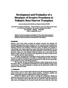
FIG. 1. Main diagram for our CADe scheme.

II.B. Scheme for nodule detection

Figure 1 shows our CADe scheme for detection of lung nodules in CXRs, which consists of five major steps: 共1兲 Segmentation of lung fields based on our M-ASM, 共2兲 our two-stage enhancement of nodules and nodule candidate detection, 共3兲 segmentation of the nodule candidates by using our clustering watershed algorithm, 共4兲 feature analysis of the segmented candidates, and 共5兲 classification of the nodule candidates into nodules or non-nodules by using a nonlinear SVM classifier. II.B.1. Segmentation of lung fields Lung segmentation is a critical component of a CADe scheme. It can prevent the occurrence of FPs outside the lung fields. Many methods have been proposed for segmenting the lungs in CXRs,39 such as 共1兲 rule-based segmentation methods, 共2兲 pixel-based methods, 共3兲 hybrid methods, and 共4兲

1847

deformable model-based methods. Because the prior information can easily be incorporated into the segmentation procedure, an active shape model 共ASM兲 has been used for lung segmentation in CXR.40–42 Because a conventional ASM cannot cover changes and variations in the entire boundaries of the lungs accurately,39 we developed a multisegment ASM 共M-ASM兲 that is adaptive to each of multiple segments of the lung boundaries 共which we call a multisegment adaptation approach兲, as illustrated in Fig. 2. Because the nodes in the conventional ASM are equally spaced along the entire lung shape, they do not fit lung shape parts with high curvatures. In our method, the model was improved by fixating of the selected nodes at specific structural boundaries which we call transitional landmarks. Transitional landmarks identified the change from one boundary type 共e.g., a boundary between the lung field and the heart兲 to another 共e.g., a boundary between the lung field and the diaphragm兲. This resulted in multiple segmented lung-field boundaries where each segment is correlated with a specific boundary type 共heart, aorta, rib cage, diaphragm, etc.兲. The node-specific ASM was built by using a fixed set of equally spaced nodes for each boundary segment. Our lung M-ASM consisted of a total of 50 nodes for each lung boundary. The nodes were not equally spaced along the entire contour. A fixed number of nodes were assigned to each boundary segment, and they were equally spaced along each boundary 共as shown in Fig. 2兲. For example, the boundary between the left lung field and the heart consisted of 11 points in every image, regardless of the actual extent of this boundary in the image 共see Fig. 2兲. This allowed the local features of nodes to fit a specific boundary segment rather than the whole lung, which resulted in a marked improvement in the accuracy of boundary segmentation. In our experiment, 93 normal images from the public JSRT database were used for training of the M-ASM. From the training images, the relative spatial relationships among the nodes in each boundary segment were learned in order to form the shape model. The nodes were arranged into a vector x and projected into the principal component shape space by means of the following expression: b = VT共x − ¯x兲,

共1兲

where V = 共V1V2 ¯ V M 兲 is the matrix of the first M eigenvectors for the shape covariance matrix and b = 共b1b2 ¯ b M 兲T is a vector of shape coefficients for the primary axes. The shape coefficients were constrained to lie in a range ⫾m冑␭i to generate only a plausible shape and projected back to node coordinates with the following expression: x = ¯x + Vb.

FIG. 2. Lung segmentation by using an M-ASM. Each blue point represents the transitional landmarks between two boundary types 共e.g., the heart and the diaphragm, the aorta, and the apex of the left lung兲. Medical Physics, Vol. 38, No. 4, April 2011

共2兲

Here, m usually has value between 2 and 3,43 and it was 2.5 in our experiment. The segmentation accuracy was computed by using the overlap measure ⍀,

1848

Chen, Suzuki, and MacMahon: A computer-aided detection scheme for lung nodule

1848

FIG. 5. Templates used for gray-level morphologic enhancement. 共a兲 Nodule template containing a bivariate normal distribution. 共b兲 Rib templates containing lines with seven different orientations.

II.B.2. Two-stage enhancement of nodules and nodule candidate detection FIG. 3. Background-trend-correction for the lung fields. 共a兲 Lung fields fitted by a second-order bivariate polynomial function. 共b兲 Preprocessed image 共background-trend-corrected image兲.

⍀=

TPseg , TPseg + FPseg + FNseg

共3兲

where TPseg was the area correctly classified as a lung field, FPseg was the area incorrectly classified as a lung field, and FNseg was the area incorrectly classified as the background. The mean and standard deviation of the overlap measure for all the 154 nodule images in the JSRT database were 0.913 and 0.023, respectively 共including the 14 images in which nodules are in the obscured lung fields兲. After the lungs were segmented, a background-trendcorrection technique was applied to the segmented lung fields. A second-order bivariate polynomial function was fitted to each of the left and right lung fields individually, as illustrated in Fig. 3共a兲, represented by F共x,y兲 = ax2 + by 2 + cxy + dx + ey + f ,

共4兲

where a, b, c, d, e, and f are coefficients, which were calculated for each case. Subsequently, the fitted functions for the left and right lung fields were subtracted from the original image. In this way, the background trend in the lung fields as a low-frequency surface was removed, as illustrated in Fig. 3共b兲. We call this image a preprocessed image.

FIG. 4. Enhancement images by using gray-level morphologic filters with a nodule template 共a兲 and rib templates 共b兲. 共a兲 Nodule-like-pattern-enhanced image. 共b兲 Rib-like-pattern-enhanced image. Medical Physics, Vol. 38, No. 4, April 2011

We developed a two-stage nodule-enhancement technique and applied it to the preprocessed image to obtain a noduleenhanced image and a nodule likelihood map. The first stage of the technique was aimed at enhancing nodules and suppressing ribs, which were a major source of FPs. Two different types of gray-level morphologic opening operators44 were used for producing a “nodule-like-pattern-enhanced” image and a “rib-like-pattern-enhanced” image. First, a gray-level morphologic opening operator with a nodule template was applied to the preprocessed image to produce a nodule-like-pattern-enhanced image, as illustrated in Fig. 4共a兲. A nodule is defined as a round opacity less than 3 cm in diameter seen in a chest radiograph,45 and it is a roughly spherical object with a density comparable to that of water, which is higher than the surrounding lung parenchyma.25 Therefore, we used a bivariate normal distribution as a nodule model in the nodule template, as shown in Fig. 5共a兲. The standard deviation of the normal distribution corresponded to the scale of the target object, i.e., the average nodule size in a database. Next, several gray-level morphologic opening operators with rib templates were applied to the preprocessed image to produce a rib-like-patternenhanced image, as illustrated in Fig. 4共b兲. Seven rib templates with seven different orientations, i.e., ⫺68°, ⫺45°, ⫺22°, 0°, +22°, +45°, and +68°, as shown in Fig. 5共b兲, were used for enhancing the riblike structures. The maximum value among the output of the seven operators was stored in each pixel in the rib-like-pattern-enhanced image. Finally, the rib-like-pattern-enhanced image was subtracted from the

FIG. 6. Nodule-enhanced image obtained by using our first-stage nodule enhancement.

1849

Chen, Suzuki, and MacMahon: A computer-aided detection scheme for lung nodule

1849

FIG. 7. Nodule enhancement by using the gray-level morphologic filter. 共a兲 ROI with a nodule. 共b兲 Enhancement of the nodule by using the gray-level morphologic filter with the nodule 共Gaussian兲 template. 共c兲 Enhancement of ribs by using the gray-level morphologic filter with the rib 共line兲 templates. 共d兲 Nodule enhanced by subtracting 共c兲 from 共b兲.

nodule-like-pattern-enhanced image to produce a noduleenhanced image, as illustrated in Fig. 6. In the image, the nodulelike patterns have larger pixel values; the riblike patterns and other patterns have smaller pixel values. The graylevel morphologic filter can enhance a nodule effectively, as demonstrated in Fig. 7. The purpose of the second stage of our nodule enhancement was to convert the nodule-enhanced image into a nodule likelihood map, as illustrated in Fig. 8. First, the noduleenhanced image was smoothed by using a Gaussian filter in order to reduce noise. Next, the gradient magnitude M ij and gradient direction Gij were calculated from the noise-reduced image by using a modified Sobel operator, represented by M ij = 冑M xij + M yij,

冤 冤

−1 0 1

Gij = arctan共M yij/M xij兲,

冥

as described below. A circle with its size related to the nodule template size was placed at an object pixel 共i , j兲, as shown in Fig. 9. The circle was divided into eight sectors numbered from 0 to 7. A nodule likelihood value for section k at the object pixel 共i , j兲 is defined by the following equation: Gkij =

1 兺 cos ␪mn , Nk mn苸sector k

t1 ⱕ M mn ⱕ t2 ,

M xij = − 2 0 2 ⴱ Inodule-enhanced , −1 0 1

M yij =

FIG. 9. Schematic diagram for our nodule likelihood calculation for a point of interest O.

1

2

1

0

0

0

−1 −2 −1

冥

共5兲

ⴱ Inodule-enhanced ,

where Inodule-enhanced is the nodule-enhanced image obtained by using the first-stage nodule enhancement. A nodule likelihood value was calculated at every pixel in the lung fields,

where ␪ is an angle between the gradient direction at a certain pixel 共m , n兲 and a vector from the object pixel 共i , j兲 to the pixel 共m , n兲, t1 and t2 are low and high gradient magnitude thresholds, respectively, and Nk is the number of pixels in sector k. When a nodule candidate is located at the object pixel 共i , j兲 and a certain pixel 共m , n兲 is on the nodule candidate, cos ␪ should be close to 1.0. Because the gradient direction is unreliable when the gradient magnitude M is small, t1 was utilized to prevent such an unreliable gradient direction from being used 共in our experiment, t1 = 5兲. t2 was utilized because a pixel 共m , n兲 may be located at a bone edge when the gradient magnitude M is large 共in our experiment, t2 = 150兲. Although some nodules have irregular shapes, the nodule likelihood values are still larger than those of ribs and other anatomic structures. The final nodule likelihood combining all sectors at the object pixel 共i , j兲 is defined by Likehoodij =

FIG. 8. Nodule likelihood map obtained by using our second-stage nodule enhancement. Medical Physics, Vol. 38, No. 4, April 2011

共6兲

¯ G ij , ␴ij

共7兲

¯ and ␴ are the mean and standard deviation, rewhere G ij ij spectively. Once a nodule likelihood map was calculated, local peaks in the map were detected. Because the smallest nodule in the JSRT database and the U of C database was larger than 5 mm, if the distance between any two peaks was less than 5 mm, a candidate was created only from the peak with the higher pixel value.

1850

Chen, Suzuki, and MacMahon: A computer-aided detection scheme for lung nodule

FIG. 10. Nodule candidate segmentation by using our clustering watershed segmentation method. 共a兲 ROI with a nodule. 共b兲 First-stage nodule enhancement image by using background-trend correction and a gray-level morphologic filter. 共c兲 Regions obtained by thresholding of the image 共b兲 with a low positive threshold value. 共d兲 Regions after erosion. 共e兲 Connected region representing a rough nodule candidate. 共f兲 Candidate region after dilation. 共g兲 Inverted image. 共h兲 Result with watershed segmentation alone. One region was divided into multiple small segments 共catchment basins兲. 共i兲 Nodule candidate segmented by our clustering watershed segmentation. 共j兲 Nodule contour.

II.B.3. Coarse-to-fine segmentation of nodule candidates After nodule candidates were detected, the boundaries of the nodule candidates had to be identified for the subsequent feature extraction. To segment the nodule candidates, we developed a “coarse-to-fine” segmentation technique based on morphologic filtering and improved watershed segmentation. First, a region of interest 共ROI兲 in which a candidate was located at the center was extracted from the nodule-enhanced image, where the size of the ROI was larger than the largest nodule to be detected 共the largest nodules in the JSRT database and the U of C database are 60 and 54 mm, respectively; in our experiment, the ROI size was 88 mm兲, as illustrated in Fig. 10共a兲. Because positive values in the noduleenhanced image are likely to be nodules, thresholding with a low positive threshold value 共pixels with values less than 5 were removed兲 was applied to the nodule-enhanced image for extraction of nodule candidate regions, as illustrated in Fig. 10共c兲. We applied a binary morphologic erosion operator to the nodule candidate regions to break connections between the nodule and non-nodule regions, as illustrated in Fig. 10共d兲. The connected region that contained the nodule candidate location 共as a point兲 determined by the initial nodule candidate detection step was retained, whereas nonnodule regions were removed, as illustrated in Fig. 10共e兲. Next, a binary morphologic dilation operator dilated the connected region. As a result, a single connected region representing a rough nodule candidate was obtained, as illustrated in Fig. 10共f兲. To refine the rough segmentation provided by morphologic filtering, we developed a clustering watershed segmentation technique. Peaks within the rough nodule candidate region in the nodule-enhanced image were obtained and used for initializing the watershed segmentation algorithm.46 For the application of watershed segmentation, the grayscale of the ROI was first inverted so that the peaks became local minima, as illustrated in Fig. 10共g兲. With the watershed segMedical Physics, Vol. 38, No. 4, April 2011

1850

FIG. 11. Criterion used for our cluster merging, where P1 and P2 are peak values in the corresponding clusters and min is the minimum value between the peaks.

mentation, the rough nodule candidate region was divided into several catchment basins. Each minimum point was surrounded by a catchment basin associated with it; thus, there were one or more peaks, each of which was surrounded by a cluster of connected pixels that constituted a catchment basin, as illustrated in Fig. 10共h兲. From the multiple catchment basins, a single nodule candidate region was determined by using the following clustering method: First, a primary cluster was defined as a cluster that contained the nodule candidate location 共as a point兲 determined by the initial nodule candidate detection step. Next, clusters connected to the primary cluster were added. The connected clusters were identified by using the criterion that the minimum value between the peak in the primary cluster and each of the other peaks was larger than a threshold value, as illustrated in Fig. 11. Figure 10共j兲 illustrates a segmented nodule candidate obtained by using the clustering watershed segmentation. II.B.4. Feature analysis and classification We extracted features from each of the segmented nodule candidates after connected-component labeling.47 Features in six categories 共i.e., shape, gray-level, surface, gradient, texture, and a specific FP兲 were extracted from the segmented candidates. The shape features were defined by the following equations: Shape1 = Aregion , Shape2 =

Shape3 =

Dmajor , Dminor Aregion Aconvex

Shape4 = 1 −

共8兲

,

hull

dcandidate-center

冑

Aregion ␲

,

where Aregion is the area of a segmented nodule candidate, Dmajor and Dminor are the long and short axes, respectively, of an ellipse that is fitted to the segmented nodule candidate, Aconvex hull is the area of the convex hull of the candidate, and dcandidate-center is the distance between the centroid of the candidate and the center of the fitted ellipse. All features were

1851

Chen, Suzuki, and MacMahon: A computer-aided detection scheme for lung nodule

Grh =

1851

1 兺 cos ␪mn , Nh mn苸regionh

t1 ⱕ M mn ⱕ t2 ,

共11兲

where Nh is the number of pixels in the segmented nodule region h. The gradient features for the segmented nodule region were given by 7

Grad1 = Gr =

冑

FIG. 12. 共a兲 Nodule region. 共b兲 Surrounding region.

Grad2 = ␴ = normalized so as to be independent of the magnification and resolution of the imaging system. The gray-level features were calculated from the segmented nodule candidates and their surrounding regions in both the preprocessed image and the nodule-enhanced image. A surrounding region was produced by subtracting a candidate region from a dilated candidate region, as illustrated in Fig. 12. The gray-level features were defined as Gray1 = ␮region − ␮surround , Gray2 = ␴region − ␴surround ,

Grad3 =

1 兺 Grh , 8 k=0 7

1 兺 共Grh − Gr兲2 , 8 k=0

共12兲

Gr . ␴

Texture features were calculated from the preprocessed image, the gradient magnitude image, and the gradient direction image, which were calculated by Eq. 共5兲. The texture features were given by the following equations: Texture1 = 兺 关C共i, j兲兴2 , ij

共9兲

Texture2 = 兺 共i − j兲2C共i, j兲,

共13兲

ij

Gray3 = minregion − minsurround ,

where C共i , j兲 is the co-occurrence matrix calculated over neighboring pixels and a summation range from the minimum to the maximum pixel value in the preprocessed image,

Gray4 = maxregion − maxsurround , where ␮, ␴, min, and max are the mean, the standard deviation, the minimum, and the maximum of pixel values in the preprocessed image, respectively, and the designation region and surround indicate a candidate region and its surrounding region, respectively. Gray5, Gray6, Gray7, and Gray8 were features calculated based on the above equations, but in the nodule-enhanced image 共instead of the preprocessed image兲. The segmented candidate region in the nodule-enhanced image was fitted to a fourth-order bivariate polynomial. The principal curvatures were calculated at the point of the highest elevation in the region. Second-order derivatives of the fitted polynomial were calculated and formed the elements of a Hessian matrix. The maximum and minimum eigenvalues of the Hessian matrix, ␭max and ␭min, were the principal curvatures. The surface features were given by Surface1 = ␭min , Surface2 = ␭max ,

共10兲

Surface3 = ␭min␭max . We used gradient in the segmented candidate region in the nodule-enhanced image to calculate gradient features, which are similar to the calculation of the nodule likelihood values in the two-stage nodule enhancement, represented by Medical Physics, Vol. 38, No. 4, April 2011

1

C共i, j兲 =

1

兺 兺 #兵f共x,y兲 = i, m=−1 n=−1

f共x + m,y + n兲 = j其

− # 兵f共x,y兲 = i, f共x,y兲 = j其,

共14兲

where # is the number of elements in the set. Texture3, Texture4, Texture5, and Texture6 are features calculated based on the above equations, but in the gradient magnitude image and the gradient direction image 共instead of the preprocessed image兲, respectively. We developed an FP reduction feature designed to eliminate rib/clavicle crossings, which are a major FP source. We used the Canny edge detector to find prominent edges within the lung field in the preprocessed image. Connected edge pixels then formed into chains which would correspond to rib/clavicle edges in the image. The overlap feature was defined by FP =

Loverlap , Lregion

共15兲

where Lregion is the length of the boundary of a candidate region and Loverlap is the number of pixels on the boundary that overlap the edge chains. In addition to the above six feature categories, segmentedcandidate-based features, Can.x, Can.y, Can.Cv1, Can.Grad1, Can.Cv2, and Can.Grad2, were calculated. Can.x and Can.y

1852

Chen, Suzuki, and MacMahon: A computer-aided detection scheme for lung nodule

FIG. 13. FROC curves indicating the performance of the nodule candidate detection part of our CADe scheme for the JSRT database and the U of C database.

are the coordinates of a nodule candidate. Can.Grad1 and Can.Grad2 are the nodule likelihood values calculated by Eq. 共7兲 at the detected nodule candidate location in the nodule candidate detection step in the nodule-enhanced image and the preprocessed image, respectively. Can.Cv1 and Can.Cv2 were calculated by using the gray-level values instead of the gradient values in Eq. 共7兲. Finally, a nonlinear SVM with a Gaussian kernel was employed for classification of the nodule candidates. We selected this classifier because its generalization ability is relatively high with a small number of training samples. We selected the Gaussian kernel among several kernels, including a polynomial kernel, because it achieved the best performance. The Gaussian kernel is represented by k共xi,x j兲 = exp共− ␦储xi − x j储2兲,

共16兲

where ␦ is a parameter. The parameter ␦ in the kernel was determined to be 1.0 by empirical analysis. Note that linear SVMs were not selected because our problem is generally a nonlinear classification problem. Classification by an SVM is realized by the solution of the following quadratic optimization problem: l

Minimize:W共a兲 = − 兺 ai + i=1

l

l

1 兺 兺 yiy jaia jk共xi,x j兲, 2 i=1 j=1

共17兲

l

Subject to

y iai = 0, 兺 i=1

∀ i:0 ⱕ ai ⱕ C,

共18兲

where l is the number of training samples and a is a vector of l variables, each component of which, ai, corresponds to a training sample 共xi , y j兲. C was determined to be l 冑兺i=1 xi · xi / l − 1.0 before training. The solution of Eq. 共17兲 is the vector aⴱ for which Eq. 共17兲 is minimized, while the constraints in Eq. 共18兲 are fulfilled. The SVM classifier was trained/tested with a leave-oneout cross-validation test. The performance of the SVM classifier was evaluated by using free-response receiverMedical Physics, Vol. 38, No. 4, April 2011

1852

FIG. 14. FROC curves indicating the performance of our CADe scheme with SVM or LDA for the JSRT database.

operating characteristic 共FROC兲 analysis48 and compared to that of a linear discriminant analysis 共LDA兲 classifier.49 Features for the LDA were selected by using the stepwise feature selection method.49 With the selection method, we determined a single set of features from M runs of a leave-one-out cross-validation test 共M is the number of features兲. Each feature was selected at each run after we accumulated all N results from the run 共N is the number of samples兲. III. RESULTS In this section, we present experimental results to demonstrate the performance of our CADe scheme. We first present the results of the initial nodule candidate detection. Then, we present the overall performance of our CADe scheme for databases BS 共a subset of the JSRT database兲, B 共the JSRT database兲, and C 共the U of C database兲. Finally, we discuss comparisons with other CADe schemes. III.A. Nodule candidate detection

The criterion for determining a TP that we adopted was that if the centroid of a detected candidate is located within the “reference-standard” nodule area, which was drawn by a radiologist, the candidate is considered as a TP. We shall call this a “region” criterion. In Sec. IV, we compare the region criterion to other criteria used in literature. Figure 13 shows the performance of the nodule candidate detection stage in our CADe scheme for the JSRT and U of C databases. The sensitivity starts dropping when the number of nodule candidates is less than 70/image. The nodule candidate detection stage in our CADe scheme achieved a sensitivity of 92.1% 共129/140兲 with 70 candidates/image and a sensitivity of 97.9% 共47/48兲 with 70 candidates/image for databases BS and C, respectively. III.B. Overall performance of the CADe scheme

FROC curves showing the overall performance of our CADe scheme for database BS 共i.e., a subset of the JRST

1853

Chen, Suzuki, and MacMahon: A computer-aided detection scheme for lung nodule

1853

TABLE III. Features selected for LDA in the two databases, i.e., databases BS 共JSRT兲 and C 共U of C兲. 共The asterisks indicate a selected feature.兲 Extracted features

JSRT

Can.x Can.y Can.Grad1 Can.Cv1 Can.Grad2 Can.Cv2 Shape1 Shape2 Shape3 Shape4

U of C

* * * * * *

*

Extracted features Gray1 Gray2 Gray3 Gray4 Gray5 Gray6 Gray7 Gray8 Grad1 Grad2

database兲 in a leave-one-out cross-validation test are shown in Fig. 14. The stepwise feature selection method selected 11 features for the LDA, as listed in Table III. The performance of our CADe scheme with the SVM was substantially higher than that of our CADe scheme with the LDA, i.e., it achieved a sensitivity of 76.4% 共107/140兲 with the SVM and a sensitivity of 60.7% with the LDA at an FP rate of 5.0 FPs/image for nodule cases in database BS. It is interesting to note that when all 31 features were used for the LDA classifier, the sensitivity was 53.6% 共75/140兲 at an FP rate of 5.0 FPs/ image for the JSRT database. It is also interesting to note that if the features selected for the LDA were used for the SVM, the performance 共i.e., a sensitivity of 68.6% 共96/140兲 with 5.0 共700/140兲 FPs/image for database BS兲 was lower than the performance of the SVM with all 31 features. This would indicate that features selected for a linear classifier are not optimal for a nonlinear classifier. The SVM-based CADe scheme marked 22 more nodules than did the LDA-based CADe scheme at an FP rate of 5 FPs/image. Most of these nodules were very subtle or extremely subtle in database BS. Table IV summarizes the performance of our CADe scheme for different databases. Figure 15 compares the performance of our CADe scheme for database BS containing all 93 normal cases and 140 nodule cases with that for the

JSRT

U of C

* * * * * *

* *

Extracted features Grad3 Surface1 Surface2 Surface3 Texture1 Texture2 Texture3 Texture4 Texture5 Texture6 FP

JSRT

U of C

*

* *

* * * * *

140 nodule cases alone. The performance for database BS was slightly higher than that for nodule cases alone. A possible reason for the higher performance is that the pessimistic bias with a leave-one-out cross-validation test was smaller when the number of cases was larger.50,51 We also included in the evaluation the 14 excluded nodules in the opaque portions of the CXR that correspond to the retrocardiac and subdiaphramatic regions of the lung, i.e., database B. The sensitivity for all 154 nodule cases 共i.e., database B兲 was lower by 9.1% 共14/154兲 than that for the 140 nodule cases because all of the 14 excluded nodules were outside the segmented lung fields; in other words, our CADe scheme did not process those areas, as designed. Figure 16 shows the performance of our CADe scheme for the U of C database 共database C兲. The stepwise feature selection method selected 12 features for the LDA, as listed in Table III. At an FP rate of 5.0 FPs/image, the sensitivity of the SVM-based CADe scheme with all 31 features was 83.3% 共40/48兲, whereas that of the LDA-based scheme with the 12 selected features was 75.0% 共36/48兲. At an FP rate of 2.0 FPs/image, the sensitivity of the SVM-based CADe scheme was 77.1% 共37/48兲.

TABLE IV. Performance of our CADe scheme for different databases for which each a classifier was trained/tested with a leave-one-out crossvalidation scheme. Databasesa

Sensitivity

FPs/image

BS

78.6% 共110/140兲 80.0% 共112/140兲b 71.4% 共100/140兲 71.4% 共110/154兲 64.9% 共100/154兲 83.3% 共40/48兲 77.1% 共37/48兲

5.0 共1165/233兲 5.0 共1165/233兲b 2.0 共466/233兲 5.0 共1235/247兲 2.0 共494/247兲 5.0 共240/48兲 2.0 共96/48兲

B C

a

Refer to Table I for details. Performance calculated with the distance criterion of 25 mm for a direct comparison with the performance in Ref. 27. Reference 24 also used the distance criterion.

b

Medical Physics, Vol. 38, No. 4, April 2011

FIG. 15. FROC curves indicating the performance of our CADe scheme for the JSRT database.

1854

Chen, Suzuki, and MacMahon: A computer-aided detection scheme for lung nodule

1854

FIG. 16. FROC curves indicating the performance of our CADe scheme for the U of C database.

FIG. 18. FROC curves indicating the performance of our CADe scheme by nodule size for the JSRT database.

We analyzed the CADe performance according to nodule subtlety, size, and pathology, as shown in Figs. 17–19 for database BS. It should be noted that the sensitivity was calculated in each category 共i.e., the sensitivity was 100% if all nodules in a particular category were marked.兲. Our CADe scheme marked 54.8% 共23/42兲 of very subtle and extremely subtle nodules with 5 FPs/image. All obvious nodules were marked with 2.6 FPs/image, and 91.9% 共35/38兲 of relatively obvious nodules were detected with 2.2 FPs/image. Our scheme has a high performance for large- and medium-sized nodules and a relatively high performance 关a sensitivity of 65.5% 共38/58兲 with 5.0 FPs/image兴 for small nodules, as shown in Fig. 18. The sensitivities for malignant and benign nodules were comparable, as shown in Fig. 19. Typical examples of our CADe detection results at operating points with FP rates of 4.5 and 4.0 FPs/image for databases BS 共i.e., the JSRT database兲 and C 共U of C database兲 are shown in Figs. 20共a兲 and 20共b兲, respectively. These examples show one TP and several FPs in each case. The FPs include an anterior and posterior rib intersection, a clavicle,

and a rib intersection. Figure 21 illustrates several examples of nodules missed by our CADe scheme. We found that the missed nodules tended to be small and to have low contrast. Most of them were rated as very or extremely subtle.

It is difficult to make definitive comparisons with the previously published CADe schemes because of different databases, different TP criteria, different evaluation procedures, different optimization parameters, and different operating points.52 We, however, attempted to compare our performance to the performance reported in literature. We found four studies in which the publicly available JSRT database was used. Table V summarizes the performance comparisons among different CADe schemes in literature. Wei et al.30 reported that their CAD scheme achieved a sensitivity of 80% with 5.4 FPs/image for the JSR database. They did not mention anything about training-testing separation. Because

FIG. 17. FROC curves indicating the performance of our CADe scheme by nodule subtlety for the JSRT database.

FIG. 19. FROC curves indicating the performance of our CADe scheme by pathology for the JSRT database.

Medical Physics, Vol. 38, No. 4, April 2011

III.C. Performance comparison with other CADe schemes

1855

Chen, Suzuki, and MacMahon: A computer-aided detection scheme for lung nodule

1855

FIG. 20. Illustrations of true positives 共arrows兲 and false positives of our CADe marks 共circles兲. 共a兲 Cases from the U of C database. 共b兲 Cases from the JSRT database.

more than 200 features 共i.e., the number of freedoms兲 were used for training and testing which were greater than the number of nodules 共i.e., the number of training samples兲 in the database, the reported performance should be highly biased due to the overtraining. Hardie et al.27 reported that their scheme marked 80% of nodules in a subset of the JSRT database 共i.e., database BS兲 with 5 FPs/image. Their performance was calculated by using the distance criterion of 25 mm for determining TP detections. Training and testing should be considered not to be independent because the authors matched the characteristics of the testing database with those of the training database. The performance 共a sensitivity of 71%兲 of our CADe scheme was substantially higher than that 共63%兲 of Hardie’s CADe scheme at a low FP setting 共2.0/image兲, which is relevant in practical use in hospitals. IV. DISCUSSION Here, we have presented a novel lung nodule CADe scheme for CXRs. A detailed performance analysis of the scheme was conducted with the use of the publicly available JSRT database 共databases BS and B兲 and our own U of C database 共database C兲. We acknowledge that many experiMedical Physics, Vol. 38, No. 4, April 2011

mental factors must be taken into account when comparisons are interpreted. However, we believe that the current scheme is certainly competitive and offers some useful innovations, including the two-stage nodule detection method and the watershed-segmentation-based feature extraction method. We made an interesting observation related to the choice of a classifier. We compared two classifiers and found that the nonlinear SVM generalized from a relatively small number of positive cases did better than did the LDA. For our CADe scheme, the SVM with all 31 extracted features provided a higher performance 共a sensitivity of 76.4% with an FP rate of 5.0 FPs/image兲 than did the LDA with selected features by the stepwise feature selection method. On the other hand, if the features selected for the LDA were used for the SVM, the performance was lower 共a sensitivity of 68.6% at 5.0 FPs/ image兲. Thus, how to select “effective” features for a particular nonlinear classifier is an important issue in CADe research. Different criteria for determining a TP have been used in different published studies. Research in Ref. 24 used a “distance” criterion that counts a detected candidate to be a TP if the distance between the centroid of the candidate and the

1856

Chen, Suzuki, and MacMahon: A computer-aided detection scheme for lung nodule

FIG. 21. Illustrations of false negatives 共arrows兲 and false positives of our CADe marks 共circles兲. 共a兲 Cases from the JSRT database. 共b兲 Cases from the U of C database.

reference-standard center of a nodule is less than 22 mm. A problem with this criterion is that the same distance is applied to nodules of any size. A “TP” region can be away from a small nodule. Research in Ref. 27 adopted a distance criterion with 25 mm as a threshold value. Research in Ref. 25 used an “overlap” criterion: A nodule is considered to be

1856

detected if there is any overlap between a detected candidate and the reference-standard region of a nodule. A detected candidate needs to be closer for being a TP for a smaller nodule than it does for a larger nodule. A problem with this criterion is that if a detected candidate region is large, the candidate that is not close enough to a nodule can be counted as a TP. The region criterion applied to our scheme evaluation is stricter than the distance criterion and the overlap criterion. We believe that the region criterion is more relevant scientifically because it does not have the problem with the distance criterion for small nodules or the problem with the “overlapping” criterion for large detected candidates, as described above. Because of the use of the stricter criterion, the measured performance of our CADe scheme could be lower than the performance measured with the other two criteria used in published studies. Schilham et al.25 reported a sensitivity of 96.4% with 134 candidates/image at the nodule candidate detection stage. This sensitivity was calculated based on the overlap criterion. Shiraishi et al.24 reported a sensitivity of 92.5% with 60.2 candidates/image based on the distance criterion. In our experiment, 3360 and 9800 nodule candidates were detected for the U of C database 共database C兲 and the JSRT database 共database BS兲, respectively. By using our region criterion, 47 and 129 true nodules were labeled as TPs for the U of C database and the JSRT database, respectively, whereas by using the distance criterion with 25 mm, 48 and 135 nodules were labeled as TPs for the U of C database and the JSRT database, respectively. Thus, the same performance was counted as a higher performance with the distance criterion than with our region criterion. Therefore, the region criterion was a stricter criterion than was the distance criterion in our experiment. In our experiment, the size of the nodule template for the two-stage nodule enhancement in the nodule candidate detection was fixed. Because the size of nodules in the JSRT database ranged from 5 to 60 mm, if we use nodule templates of different sizes adaptively for different-sized nodules, the performance of the initial nodule candidate detection can be improved. The development of such a method is planned for our future study. We analyzed the false-negative nodules at the sensitivity of 76% in the JSRT database. We found that they were lo-

TABLE V. Performance comparisons of CADe schemes that used the JSRT database for evaluation in literature. Sensitivity

FPs/image

Database

Wei et al. 共2002兲 共Ref. 30兲

80% 共123/154兲

5.4 共1333/247兲

Coppini et al. 共2003兲 共Ref. 23兲 Schilham et al. 共2006兲 共Ref. 25兲

60% 共93/154兲 51% 共79/154兲 67% 共103/154兲 80% 共112/140兲 63% 共88/140兲

4.3 2.0 4.0 5.0 2.0

All nodule and normal cases in JSRT 共247兲 All nodules cases in JSRT 共154兲 All nodule cases in JSRT 共154兲

a

Hardie et al. 共2009兲 共Ref. 27兲b

共662/154兲 共308/154兲 共616/154兲 共700/140兲 共280/140兲

Nodule cases in JSRT 共140兲

The authors did not discuss training-testing separation. More than 200 features 共i.e., the number of freedoms兲 were used for training and testing, which were greater than the number of nodules 共i.e., the number of training samples兲 in the database. b Performance was calculated by using the distance criterion of 25 mm for determining TP detections. a

Medical Physics, Vol. 38, No. 4, April 2011

1857

Chen, Suzuki, and MacMahon: A computer-aided detection scheme for lung nodule

cated either in the pulmonary trunk and artery areas or behind ribs and/or clavicles. Because of these complex backgrounds, our scheme was not able to produce accurate segmentation of the nodules. As a result, the features computed in the subsequent step were less accurate, and this made the classification task more difficult. In the evaluation of our CADe scheme, we used the publicly available JSRT database. A good feature of this database is that the observer performance study results for radiologists are available. The study showed that radiologists detected only 44% of the extremely and very subtle cases. At an FP rate of 5.0 FPs/image, our CADe scheme correctly detected 55% of these cases in the same category, whereas a conventional CADe scheme, reported in Ref. 25, detected 41% of the cases. This is encouraging because our CADe scheme has a desirable characteristic, which is a high sensitivity for subtle cases. Therefore, we expect that our CADe scheme will potentially be useful for improving radiologists’ performance in the detection of subtle nodules. The performance of our CADe scheme was higher for the U of C database than for the JSRT database. The reasons for this are threefold: 共1兲 Nodules in the JSRT database were more subtle than those in the U of C database. There were 42 very subtle and extremely subtle nodules out of 140 nodules in the JSRT database. There are “nonactionable” nodules where all of 6 expert radiologists did not detect even when they were marked by a hypothetical CADe scheme with 100% sensitivity in an observer performance study.53 共2兲 The average size of the nodules in the U of C database was larger than that in the JSRT database. 共3兲 The images in the U of C database were digital images acquired with a computed radiography system, whereas the images in the JSRT database were digitized images scanned from films. Thus, the quality of images in the U of C database was better than that of the images in the JSRT database. Therefore, the “difficulty” of databases was substantially different. This substantial difference in database characteristics may have caused the different feature sets selected for LDA with the stepwise feature selection method. How much a CADe scheme is able to improve the performance of a radiologist depends on the following factors: Radiologist’s experience, “stand-alone” performance of the CADe scheme, and the ability of the reader to distinguish a TP marking from a FP marking.14 We have developed a CADe scheme that achieved a relatively high performance. We expect that the higher stand-alone performance will be beneficial to the improvement of radiologist’s performance. We will need to carry out an observer performance study with radiologists to prove this. The time for processing one case with our CADe scheme was about 70 s 共including 25 s for nodule candidate detection and 45 s for candidate segmentation, feature extraction, and classification兲 on a PC-based workstation 共Intel Pentium 2.4 GHz processor with a 3 GB memory兲. The candidate segmentation consumed about half of the entire processing time. Thus, CADe results will be obtained 70 s after the acquisiMedical Physics, Vol. 38, No. 4, April 2011

1857

tion of a CXR. Therefore, at the time of the radiologist’s reading, CADe results will already be available on a viewing workstation for his/her review. V. CONCLUSION We have developed a CADe scheme for the detection of lung nodules in CXRs. Our CADe scheme consists of an accurate lung segmentation based on the multisegment ASM, a new two-stage nodule-enhancement technique, nodule segmentation by using an improved watershed segmentation, and an SVM classifier. Our CADe scheme achieved sensitivities of 76% 共107/140兲 and 77% 共37/48兲 with 5.0 共700/ 140兲 FPs/image and 2.0 共96/48兲 FPs/image for a publicly available database 共JSRT兲 and our database 共U of C兲, respectively, in a leave-one-out cross-validation test. Therefore, we expect that our CADe scheme will be potentially useful for improving radiologist’s sensitivity in the detection of lung nodules in chest radiographs. ACKNOWLEDGMENTS The authors are grateful to Dr. M. L. Giger for her valuable suggestions, E. F. Lanzl for improving the manuscript, and to Riverain Medical for research support. This work was supported partially by Grant No. R01CA120549 from the National Cancer Institute/National Institutes of Health and by NIH S10 RR021039 and P30 CA14599. CAD technologies developed at the University of Chicago have been licensed to companies including R2 Technology 共Hologic兲, Riverain Medical, Deus Technology, Median Technologies, Mitsubishi Space Software, General Electric, and Toshiba. a兲

Author to whom correspondence should be addressed. Electronic addresses: [email protected] and [email protected]; Telephone: 共773兲 834-5098; Fax: 共773兲 702-0371. 1 American Cancer Society, American Cancer Society Complete Guide to Complementary & Alternative Cancer Therapies, 2nd ed. 共American Cancer Society, Atlanta, GA, 2009兲. 2 J. V. Forrest and P. J. Friedman, “Radiologic errors in patients with lung cancer,” West. J. Med. 134共6兲, 485–490 共1981兲. 3 C. I. Henschke et al., “Early lung cancer action project: Overall design and findings from baseline screening,” Lancet 354共9173兲, 99–105 共1999兲. 4 G. P. Murphy et al., American Cancer Society Textbook of Clinical Oncology, 2nd ed. 共The Society, Atlanta, GA, 1995兲. 5 G. Revesz, H. L. Kundel, and M. A. Graber, “The influence of structured noise on the detection of radiologic abnormalities,” Invest. Radiol. 9共6兲, 479–486 共1974兲. 6 R. S. Fontana et al., “The Mayo Lung Project for early detection and localization of bronchogenic carcinoma: A status report,” Chest 67共5兲, 511–522 共1975兲. 7 H. L. Kundel and G. Revesz, “Lesion conspicuity, structured noise, and film reader error,” AJR, Am. J. Roentgenol. 126共6兲, 1233–1238 共1976兲. 8 J. H. Austin, B. M. Romney, and L. S. Goldsmith, “Missed bronchogenic carcinoma: Radiographic findings in 27 patients with a potentially resectable lesion evident in retrospect,” Radiology 182共1兲, 115–122 共1992兲. 9 P. K. Shah et al., “Missed non-small cell lung cancer: Radiographic findings of potentially resectable lesions evident only in retrospect,” Radiology 226共1兲, 235–241 共2003兲. 10 M. L. Giger, K. Doi, and H. MacMahon, “Image feature analysis and computer-aided diagnosis in digital radiography. 3. Automated detection of nodules in peripheral lung fields,” Med. Phys. 15共2兲, 158–166 共1988兲. 11 B. Van Ginneken, B. M. ter Haar Romeny, and M. A. Viergever, “Computer-aided diagnosis in chest radiography: A survey,” IEEE Trans. Med. Imaging 20共12兲, 1228–1241 共2001兲.

1858

Chen, Suzuki, and MacMahon: A computer-aided detection scheme for lung nodule

12

T. Kobayashi et al., “Effect of a computer-aided diagnosis scheme on radiologists’ performance in detection of lung nodules on radiographs,” Radiology 199共3兲, 843–848 共1996兲. 13 H. MacMahon et al., “Computer-aided diagnosis of pulmonary nodules: Results of a large-scale observer test,” Radiology 213共3兲, 723–726 共1999兲. 14 D. W. De Boo et al., “Computer-aided detection 共CAD兲 of lung nodules and small tumours on chest radiographs,” Eur. J. Radiol. 72共2兲, 218–225 共2009兲. 15 M. L. Giger et al., “Computerized detection of pulmonary nodules in digital chest images: Use of morphological filters in reducing falsepositive detections,” Med. Phys. 17共5兲, 861–865 共1990兲. 16 S.C. Lo, M. T. Freedman, J. S. Lin, and S. K. Mun, “Automatic lung nodule detection using profile matching and back-propagation neural network techniques,” J. Digit Imaging 6共1兲, 48–54 共1993兲. 17 S.-C. B. Lo et al., “Artificial convolution neural network techniques and applications to lung nodule detection,” IEEE Trans. Med. Imaging 14共4兲, 711–718 共1995兲. 18 X. W. Xu et al., “Development of an improved CAD scheme for automated detection of lung nodules in digital chest images,” Med. Phys. 24共9兲, 1395–1403 共1997兲. 19 H. Yoshida et al., “Computer-aided diagnosis scheme for detecting pulmonary nodules using wavelet transform,” Proceedings of SPIE Medical Imaging: Image Processing, Vol. 2434, pp. 621–626, 1995 共unpublished兲. 20 N. F. Vittitoe, J. A. Baker, and C. E. Floyd, Jr., “Fractal texture analysis in computer-aided diagnosis of solitary pulmonary nodules,” Acad. Radiol. 4共2兲, 96–101 共1997兲. 21 M. J. Carreira et al., “Computer-aided diagnoses: Automatic detection of lung nodules,” Med. Phys. 25共10兲, 1998–2006 共1998兲. 22 M. G. Penedo et al., “Computer-aided diagnosis: A neural-network-based approach to lung nodule detection,” IEEE Trans. Med. Imaging 17共6兲, 872–880 共1998兲. 23 G. Coppini et al., “Neural networks for computer-aided diagnosis: Detection of lung nodules in chest radiograms,” IEEE Trans. Inf. Technol. Biomed. 7共4兲, 344–357 共2003兲. 24 J. Shiraishi et al., “Computer-aided diagnostic scheme for the detection of lung nodules on chest radiographs: Localized search method based on anatomical classification,” Med. Phys. 33共7兲, 2642–2653 共2006兲. 25 A. M. Schilham, B. van Ginneken, and M. Loog, “A computer-aided diagnosis system for detection of lung nodules in chest radiographs with an evaluation on a public database,” Med. Image Anal. 10共2兲, 247–258 共2006兲. 26 P. Campadelli, E. Casiraghi, and D. Artioli, “A fully automated method for lung nodule detection from postero-anterior chest radiographs,” IEEE Trans. Med. Imaging 25共12兲, 1588–1603 共2006兲. 27 R. C. Hardie et al., “Performance analysis of a new computer aided detection system for identifying lung nodules on chest radiographs,” Med. Image Anal. 12共3兲, 240–258 共2008兲. 28 F. Mao et al., “Fragmentary window filtering for multiscale lung nodule detection: Preliminary study,” Acad. Radiol. 5共4兲, 306–311 共1998兲. 29 Q. Li, S. Katsuragawa, and K. Doi, “Computer-aided diagnostic scheme for lung nodule detection in digital chest radiographs by use of a multipletemplate matching technique,” Med. Phys. 28共10兲, 2070–2076 共2001兲. 30 J. Wei et al., “Optimal image feature set for detecting lung nodules on chest x-ray images,” Computer Assisted Radiology and Surgery 共Springer, Paris, 2002兲, pp. 706–711. 31 M. Freedman et al., “Computer-aided detection of lung cancer on chest radiographs: Effect of machine CAD true positive/false negative detections on radiologist’s confidence level,” Proceedings of SPIE Medical Imaging: Image Processing, Vol. 5372, pp. 185–191, 2004 共unpublished兲. 32 T. Matsumoto et al., “Potential usefulness of computerized nodule detection in screening programs for lung cancer,” Invest. Radiol. 27共6兲, 471–

Medical Physics, Vol. 38, No. 4, April 2011

1858

475 共1992兲. B. Keserci and H. Yoshida, “Computerized detection of pulmonary nodules in chest radiographs based on morphological features and wavelet snake model,” Med. Image Anal. 6共4兲, 431–447 共2002兲. 34 H. Yoshida, “Multiscale edge-guided wavelet snake model for delineation of pulmonary nodules in chest radiographs,” J. Electron. Imaging 12共1兲, 69–80 共2003兲. 35 H. Yoshida, “Local contralateral subtraction based on bilateral symmetry of lung for reduction of false positives in computerized detection of pulmonary nodules,” IEEE Trans. Biomed. Eng. 51共5兲, 778–789 共2004兲. 36 K. Suzuki et al., “False-positive reduction in computer-aided diagnostic scheme for detecting nodules in chest radiographs by means of massive training artificial neural network,” Acad. Radiol. 12共2兲, 191–201 共2005兲. 37 J. Shiraishi et al., “Development of a digital image database for chest radiographs with and without a lung nodule: Receiver operating characteristic analysis of radiologists’ detection of pulmonary nodules,” AJR, Am. J. Roentgenol. 174共1兲, 71–74 共2000兲. 38 J. A. Swets, “ROC analysis applied to the evaluation of medical imaging techniques,” Invest. Radiol. 14共2兲, 109–121 共1979兲. 39 Y. Shi et al., “Segmenting lung fields in serial chest radiographs using both population-based and patient-specific shape statistics,” IEEE Trans. Med. Imaging 27共4兲, 481–494 共2008兲. 40 T. F. Cootes et al., “Use of active shape models for locating structures in medical images,” Image Vis. Comput. 12共6兲, 355–365 共1994兲. 41 B. van Ginneken, M. B. Stegmann, and M. Loog, “Segmentation of anatomical structures in chest radiographs using supervised methods: A comparative study on a public database,” Med. Image Anal. 10共1兲, 19–40 共2006兲. 42 D. Seghers et al., “Minimal shape and intensity cost path segmentation,” IEEE Trans. Med. Imaging 26共8兲, 1115–1129 共2007兲. 43 B. van Ginneken et al., “Active shape model segmentation with optimal features,” IEEE Trans. Med. Imaging 21共8兲, 924–933 共2002兲. 44 J. Serra, Image Analysis and Mathematical Morphology 共Academic Press, Orlando, 1982兲, Vol. 1. 45 J. H. Austin et al., “Glossary of terms for CT of the lungs: Recommendations of the Nomenclature Committee of the Fleischner Society,” Radiology 200共2兲, 327–331 共1996兲. 46 L. Vincent and P. Soille, “Watersheds in digital spaces: An efficient algorithm based on immersion simulations,” IEEE Trans. Pattern Anal. Mach. Intell. 13共6兲, 583–598 共1991兲. 47 K. Suzuki, I. Horiba, and N. Sugie, “Linear-time connected-component labeling based on sequential local operations,” Comput. Vis. Image Underst. 89共1兲, 1–23 共2003兲. 48 D. Chakraborty, “Maximum likelihood analysis of free-response receiver operating characteristic 共FROC兲 data,” Med. Phys. 16, 561–568 共1989兲. 49 B. Sahiner et al., “Feature selection and classifier performance in computer-aided diagnosis: The effect of finite sample size,” Med. Phys. 27共7兲, 1509–1522 共2000兲. 50 B. Sahiner, H. P. Chan, and L. Hadjiiski, “Classifier performance estimation under the constraint of a finite sample size: Resampling schemes applied to neural network classifiers,” Neural Networks 21共2–3兲, 476– 483 共2008兲. 51 B. Sahiner, H. P. Chan, and L. Hadjiiski, “Classifier performance prediction for computer-aided diagnosis using a limited dataset,” Med. Phys. 35共4兲, 1559–1570 共2008兲. 52 R. M. Nishikawa et al., “Effect of case selection on the performance of computer-aided detection schemes,” Med. Phys. 21共2兲, 265–269 共1994兲. 53 J. Shiraishi et al., “Effect of high sensitivity in a computerized scheme for detecting extremely subtle solitary pulmonary nodules in chest radiographs: Observer performance study,” Acad. Radiol. 10共11兲, 1302–1311 共2003兲. 33