ns2 simulator) numerous test conditions using CBR and TCP traffic and compared ... Also, a comparison of some performance metrics for TCP and CBR.
Development and Performance Characterization of Enhanced AODV Routing for CBR and TCP Traffic by
PRADEEPKUMAR MANI Bachelor of Engineering, Electrical and Electronics Engineering Anna University Chennai, India, 2001.
Submitted to the Department of Electrical Engineering and Computer Science and the Faculty of the Graduate School of the University of Kansas in partial fulfillment of the requirements for the degree of Master of Science
Thesis Committee:
Dr. David W. Petr: Chairperson
Dr. Joseph B. Evans
Dr. Victor S. Frost
Date Submitted: ________________
Dedicated to my parents, my brother and my fiancée
ii
Abstract This thesis aims to modify an existing mobile ad-hoc network (MANET) reactive routing protocol (AODV) into a hybrid protocol by introducing adaptive, proactive behavior to improve its performance. Under our proposed scheme, route maintenance decisions are based on predicted values of 'link-breakage times' (when the next-hop node will move out of transmission range) obtained from a series of position/velocity estimates of the nexthop node. These estimates are based on the power level of the received MAC frames. If a link is about to break, proactive discovery of new routes to all destinations using the nexthop node depends on the history of traffic to that destination. We simulated (using the ns2 simulator) numerous test conditions using CBR and TCP traffic and compared performance metrics for the original and modified versions of the protocol. We were able to achieve (1) a significant reduction in mean packet latency for CBR traffic and (2) a reduction in control overhead in TCP traffic, while incurring other small penalties for both types of traffic. Also, a comparison of some performance metrics for TCP and CBR traffic led us to conclude that slight modifications in TCP can lead to its improved performance over MANETs.
iii
Acknowledgements First of all, I would like to thank my advisor and my committee chair, Dr. David W. Petr, for his invaluable guidance and timely input provided throughout the duration of this thesis work. I am indebted to him for funding me throughout my graduate studies and for allowing me to choose the area of research for my thesis work. His constant motivation and support has helped me perform better not only in research but also in my graduate coursework. His excellent teaching has equipped me with sound fundamentals in communication network analysis and integrated telecommunication networks. I have learnt a lot about simulation-based research by working under him. I am very grateful to him for all the time he has had to spare for the numerous discussions we have had regarding my future plans.
I would like to thank Dr. Evans for serving in my thesis committee and for providing me with the opportunity to work with MANETs in my directed graduate reading course. This course provided me exposure to research in MANETs, which helped me decide on my area of research. I would also like to thank Dr. Frost for serving in my thesis committee. I would also like express my gratitude to all the technical and administrative staff at ITTC for their support.
I would like to thank all my friends with whom I have had a wonderful time in the past and in the present. A special thanks to my parents, my brother and my fiancée for being there for me and providing me with all the encouragement I needed. Finally, I would like to thank GOD for all the blessings without which none of this would have been possible.
iv
Table of Contents Chapter 1 Introduction....................................................... 1 1.1 MOTIVATION.............................................................................................................. 2 1.2 RESEARCH OVERVIEW ............................................................................................... 2 1.3 ORGANIZATION OF THESIS ......................................................................................... 4
Chapter 2 Background ....................................................... 5 2.1 INTRODUCTION .......................................................................................................... 5 2.2 ROUTING PROTOCOLS FOR MANETS ........................................................................ 6 2.2.1 Table Driven or Proactive Protocols ............................................................................. 7 2.2.1.1 Destination Sequenced Distance Vector Routing .................................................................7
2.2.2 On-Demand or Reactive Protocols ................................................................................ 9
2.3
2.2.2.1 Dynamic Source Routing ....................................................................................................10 2.2.2.2 Ad-hoc On-Demand Distance Vector Routing (AODV) ....................................................13 2.2.2.3 Signal Stability-Based Adaptive Routing (SSA).................................................................15 DISCUSSION OF TABLE-DRIVEN VS. ON-DEMAND ROUTING PROTOCOLS ................ 17
Chapter 3 Link Lifetime Prediction Algorithm................. 19 3.1 INTRODUCTION ........................................................................................................ 19 3.2 RADIO PROPAGATION MODEL.................................................................................. 19 3.3 PREDICTION ALGORITHMS ........................................................................................ 21 3.3.1 Details of Prediction algorithm ................................................................................... 22
3.4 DISCUSSION ............................................................................................................. 25
Chapter 4 Protocol Design and Implementation.............. 27 4.1 PROTOCOL CHOICE ................................................................................................... 27 4.1.1 Hybrid Protocol ........................................................................................................... 27
4.2 PROTOCOL IMPLEMENTATION DETAILS ................................................................... 28 4.2.1 MAC layer Implementation .......................................................................................... 28 4.2.2 AODV layer Implementation........................................................................................ 30
4.3
4.2.2.1 Active Routes in AODV .....................................................................................................30 4.2.2.2 Proactive Route Discovery..................................................................................................32 4.2.2.3 Replacing a ‘broken’ route..................................................................................................32 DISCUSSION ............................................................................................................. 33
Chapter 5 Evaluation ....................................................... 35 5.1 INTRODUCTION ........................................................................................................ 35 5.2 SIMULATOR CHOICE ................................................................................................ 35 5.2.1 NS-2 basics................................................................................................................... 36
5.3 PERFORMANCE METRICS ......................................................................................... 37 5.4 SIMULATION DETAILS .............................................................................................. 38 5.4.1 Simulations with UDP traffic ....................................................................................... 39 5.4.1.1 Simulations with Random Waypoint Model .......................................................................39 5.4.1.1.1 Simulation Results ................................................................................................................. 41
5.4.1.2 Simulation parameters for Manhattan Grid Model: ............................................................53 5.4.1.2.1 Simulation Results ................................................................................................................. 55
v
5.4.2 Simulations with TCP traffic........................................................................................ 61 5.4.2.1 Simulations with Random Waypoint Model .......................................................................62 5.4.2.1.1 Simulation Results ................................................................................................................. 62
5.4.2.2 Simulation parameters for Manhattan Grid Model: ............................................................70 5.4.2.2.1 Simulation Results ................................................................................................................. 70
5.4.3 Comparison of CBR and TCP results .......................................................................... 77
5.5 CONCLUSIONS .......................................................................................................... 80
Chapter 6 Conclusions and Future work ......................... 81 6.1 SUMMARY OF WORK DONE ....................................................................................... 81 6.2 CONCLUSIONS .......................................................................................................... 81 6.3 FUTURE WORK ........................................................................................................ 82
References ........................................................................ 84 Appendix........................................................................... 87
vi
List of Figures FIGURE 2-1 A MANET OF 3 NODES .................................................................................................. 5 FIGURE 2.2 CLASSIFICATION OF MANET ROUTING PROTOCOLS ................................................... 7 FIGURE 2.3 ROUTE DISCOVERY PROCESS IN DSR ......................................................................... 11 FIGURE 3.1 SCHEMATIC FOR SIMPLE PREDICTION MODEL USING GPS .......................................... 22 FIGURE 4.1 INTERACTION BETWEEN EAODV AND AODV ROUTE MAINTENANCE ...................... 34 FIGURE 5.4.1.1 E2E VS MAX VELOCITY (RW MODEL, CBR TRAFFIC).......................................... 43 FIGURE 5.4.1.2 E2E VS PAUSE TIME (RW MODEL, CBR TRAFFIC)................................................ 43 FIGURE 5.4.1.3 E2E VS MEAN PACKET INTER-ARRIVAL TIME (RW MODEL, CBR TRAFFIC) ........ 44 FIGURE 5.4.1.4 P.D.R VS MAX VELOCITY (RW MODEL, CBR TRAFFIC) ....................................... 46 FIGURE 5.4.1.5 P.D.R VS PAUSE TIME (RW MODEL, CBR TRAFFIC) ............................................. 47 FIGURE 5.4.1.6 P.D.R VS MEAN PACKET INTER-ARRIVAL TIME (RW MODEL, CBR TRAFFIC)...... 47 FIGURE 5.4.1.7 C.P.D VS MAX VELOCITY (RW MODEL, CBR TRAFFIC) ....................................... 49 FIGURE 5.4.1.8 C.P.D VS PAUSE TIME (RW MODEL, CBR TRAFFIC) ............................................. 49 FIGURE 5.4.1.9 C.P.D VS MEAN PACKET INTER-ARRIVAL TIME (RW MODEL, CBR TRAFFIC)...... 50 FIGURE 5.4.1.10 HOPS VS MAX VELOCITY (RW MODEL, CBR TRAFFIC) ..................................... 52 FIGURE 5.4.1.12 HOPS VS MEAN PACKET INTER-ARRIVAL TIME (RW MODEL, CBR TRAFFIC) .... 52 FIGURE 5.4.1.13 E2E VS TURN PROBABILITY (MG MODEL, CBR TRAFFIC) .................................. 56 FIGURE 5.4.1.14 E2E VS PAUSE PROBABILITY (MG MODEL, CBR TRAFFIC) ................................. 57 FIGURE 5.4.1.15 P.D.R VS TURN PROBABILITY (MG MODEL, CBR TRAFFIC) ................................ 58 FIGURE 5.4.1.16 P.D.R VS PAUSE PROBABILITY (MG MODEL, CBR TRAFFIC)............................... 59 FIGURE 5.4.1.17 C.P.D VS TURN PROBABILITY (MG MODEL, CBR TRAFFIC) ................................ 59 FIGURE 5.4.1.18 C.P.D VS PAUSE PROBABILITY (MG MODEL, CBR TRAFFIC)............................... 60 FIGURE 5.4.1.19 HOPS VS TURN PROBABILITY (MG MODEL, CBR TRAFFIC) ................................ 60
vii
FIGURE 5.4.1.20 HOPS VS PAUSE PROBABILITY (MG MODEL, CBR TRAFFIC)............................... 61 FIGURE 5.4.2.1 C.P.D VS MAX VELOCITY (RW MODEL, TCP TRAFFIC) ........................................ 65 FIGURE 5.4.2.2 C.P.D VS PAUSE TIME (RW MODEL, TCP TRAFFIC) .............................................. 66 FIGURE 5.4.2.3 THROUGHPUT VS MAX VELOCITY (RW MODEL, TCP TRAFFIC) .......................... 66 FIGURE 5.4.2.4 THROUGHPUT VS PAUSE TIME (RW MODEL, TCP TRAFFIC) ................................ 67 FIGURE 5.4.2.5 E2E VS MAX VELOCITY (RW MODEL, TCP TRAFFIC) .......................................... 67 FIGURE 5.4.2.6 E2E VS PAUSE TIME (RW MODEL, TCP TRAFFIC)................................................. 68 FIGURE 5.4.2.7 HOPS VS MAX VELOCITY (RW MODEL, TCP TRAFFIC) ........................................ 68 FIGURE 5.4.2.8 HOPS VS PAUSE TIME (RW MODEL, TCP TRAFFIC) .............................................. 69 FIGURE 5.4.2.9 C.P.D VS TURN PROBABILITY (MG MODEL, TCP TRAFFIC)................................... 72 FIGURE 5.4.2.10 C.P.D VS PAUSE PROBABILITY (MG MODEL, TCP TRAFFIC) ............................... 73 FIGURE 5.4.2.11 THROUGHPUT VS TURN PROBABILITY (MG MODEL, TCP TRAFFIC) .................. 73 FIGURE 5.4.2.12 THROUGHPUT VS PAUSE PROBABILITY (MG MODEL, TCP TRAFFIC) ................. 74 FIGURE 5.4.2.13 E2E VS TURN PROBABILITY (MG MODEL, TCP TRAFFIC) ................................... 74 FIGURE 5.4.2.14 E2E VS PAUSE PROBABILITY (MG MODEL, TCP TRAFFIC).................................. 75 FIGURE 5.4.2.15 HOPS VS TURN PROBABILITY (MG MODEL, TCP TRAFFIC)................................. 75 FIGURE 5.4.2.16 HOPS VS PAUSE PROBABILITY (MG MODEL, TCP TRAFFIC) ............................... 76 FIGURE 5.4.3.1 NUMBER OF TCP PACKETS VS TIME ..................................................................... 79 FIGURE 5.4.3.2 NUMBER OF CBR PACKETS VS TIME .................................................................... 79
viii
List of Tables TABLE 2.1 ON-DEMAND VS. TABLE-DRIVEN ROUTING PROTOCOLS .............................................. 18 TABLE 5.4.1.1 STATISTICAL PARAMETER VALUES FOR VARIOUS RW MOBILITY PATTERNS ....... 41 TABLE 5.4.1.2 STATISTICAL PARAMETER VALUES FOR VARIOUS MG MOBILITY PATTERNS ....... 55
ix
Chapter 1 Introduction Recent advances in wireless communication technologies and availability of less expensive computer processing power have led to a surge in interest in mobile computing and its applications. A "mobile ad hoc network" (MANET) is an autonomous system of mobile routers (and associated hosts) connected by wireless links - the union of which forms an arbitrary graph. The routers are free to move randomly and organize themselves arbitrarily; thus, the network’s wireless topology may change rapidly and unpredictably. Such a network may operate in a standalone fashion, or may be connected to the larger Internet [1]. Applications of MANETs are aplenty - some examples include military use in battle fields, where a centralized command center is not only infeasible but also undesirable; and disaster management scenarios, where communication between various rescue teams is required in the absence of any existing communication infrastructure.
A key challenge in MANETs is to devise efficient methods to ensure route availability while incurring minimal control overhead. MANET routing protocols are of two kinds: proactive (table-driven) and reactive (on-demand). Proactive protocols always have routes to any destination in the network, while reactive protocols need to discover routes as needed. Proactive protocols suffer from excessive control overhead associated with maintaining routes to destinations even when not required, while reactive protocols experience higher end-to-end packet delays when compared to proactive protocols. Examples of proactive protocols are Destination Sequenced Distance Vector (DSDV) [2] and Optimized Link State Routing (OLSR) [3] while some examples of reactive protocols include Dynamic Source Routing (DSR) [4], Ad hoc On-demand Distance Vector 1
(AODV) routing [5] etc. A third class of protocols, Hybrid Protocols, imbibes the qualities of both proactive and reactive protocols. One example of a hybrid protocol is the Zone Routing Protocol (ZRP) [6].
1.1 Motivation Ideally, a routing protocol that produces routing overhead comparable to a reactive protocol and offers end-to-end packet delays comparable to a proactive protocol is desired. End-to-end packet latency is an important consideration in real time applications like voice, video etc, which are time critical. In the near future, one can expect a significant amount of multimedia traffic in ad hoc networks. Conventional ad hoc protocols are not capable of handling real time traffic. The work described here is an attempt to design a routing protocol that offers lesser end-to-end packet delays for realtime traffic and lesser control overhead for TCP traffic. This can only be achieved by tapping link state information, which is generally ignored in conventional ad hoc routing protocols. Existing hybrid protocols do not make use of link state information, and hence do not offer a great performance advantage over existing reactive or proactive protocols; each protocol performs better in certain scenarios.
1.2 Research Overview The scope of this research is to provide extensions to an existing reactive ad hoc routing protocol (AODV) in the form of cross-layer interaction capabilities along with a prediction algorithm to predict link breakage times. Further, the reactive protocol is
2
modified into an adaptive, hybrid protocol by suitably modifying the route maintenance procedure in AODV to introduce selective proactivity. We call the resulting protocol Enhanced AODV (EAODV). The following presents a summary of the total work done:
1. Developed a prediction algorithm to predict link breakage time from signal strength information extracted from a packet received on that particular logical link 2. At the MAC layer, introduced a table of link-to-neighbor breakage times of logical links associated with the particular mobile node, and provided an interface for upper layers to access this table 3. Provided methods to assess the state of any link as ACTIVE or IDLE 4. At the AODV layer, provided methods to assess the state of each route as ACTIVE or IDLE 5. Through the interface provided at the MAC layer, used the available link state information to make intelligent, proactive AODV route maintenance decisions for ACTIVE routes only. 6. Implemented the above enhancements to AODV and 802.11 MAC in the ns-2 simulator and ran simulations for thorough performance evaluation studies to compare AODV and Enhanced AODV (EAODV) 7. For CBR traffic, achieved a significant reduction in mean end-to-end packet latency at a small cost in the form of a marginal increase in control overhead and a marginal decrease in packet delivery ratio
3
8. For TCP traffic, achieved a significant reduction in percentage routing control overhead at a small cost in the form of a marginal reduction in TCP throughput. 9. Realized the need for modifications to TCP to increase TCP throughput in ad hoc networks.
1.3 Organization of Thesis This thesis is organized as follows: Chapter (2) is an introduction to mobile ad hoc networks and some of the existing reactive, proactive and hybrid protocols. Some results from published works are discussed as well. Chapter (3) presents the prediction algorithm in detail. Chapter (4) gives a brief introduction to the network simulator (ns-2) and deals with implementation details of the prediction algorithm and cross-layer capabilities. Chapter (5) details the performance metrics chosen, simulation scenarios and results of simulations. Chapter (6) discusses conclusions drawn from simulation experiments and scope for future work.
4
Chapter 2 Background 2.1 Introduction A Mobile Ad Hoc Network generally does not have any infrastructure and each mobile host also acts as a router. Communication between various hosts takes place through wireless links. Direct communication can take place between hosts that are within the communication range of the antennas of the respective hosts; otherwise, communication is achieved through multi-hop routing. Figure 2.1 represents a MANET of 3 nodes. Node 2 can communicate directly with Node 1 and Node 3. But any communication between Nodes 1 and 3 must be routed through Node 2.
1
2
3
Figure 2-1 A Manet of 3 Nodes
A major part of this chapter is based on [7]. The following are the salient features of MANETs: •
Dynamic Topologies: All nodes in the MANET generally move with varying velocities, and hence the network topology changes dynamically. Frequent link breaks are quite common. New nodes may join the network or existing nodes can leave the network. The dynamic changes in the network topology pose the biggest challenge to routing in Ad Hoc Networks.
5
•
Asymmetrical Communication: Each node in the Ad Hoc Network may have antennas of different characteristics, and hence symmetrical, bi-directional communication over the same link is not always possible. In some cases, only unidirectional communication is possible.
•
Bandwidth limitations: Since the nodes communicate via wireless links, the realized throughput in these networks when compared to a wired network of similar size is quite small. The relatively lower capacity of the wireless links does not facilitate transmission of delay-constrained traffic (real-time or multimedia traffic). Moreover, the wireless links are quite error-prone, which may further degrade throughput due to upper layer retransmissions, etc.
•
Energy limitations: The nodes in the MANET are generally battery operated. Hence, energy conservation techniques and energy-aware routing in MANETs become necessary.
Existing routing protocols in wired networks (both link state and distance vector) are not suitable for MANETs. These routing protocols distribute topological information across the network to update other nodes of topological changes. This mechanism is not suitable in MANETs, because there are frequent topological changes as the nodes move randomly causing frequent link breakages.
2.2 Routing Protocols for MANETs The existing routing protocols in MANETs can be classified into two categories: (1) Table-driven routing protocols, and (2) On-demand routing protocols. Fig 2.2 shows the classification along with some examples of existing MANET protocols.
6
Figure 2.2 Classification of MANET Routing Protocols
2.2.1 Table Driven or Proactive Protocols Table-driven protocols (proactive protocols) generate frequent updates of network topology information to maintain a consistent view of the network at all nodes. These nodes are required to maintain tables containing topology information, so that any node wishing to communicate with any other node may do so by computing a route to the destination node from the table. It is fairly expensive in terms of table size and control overhead to maintain a table of topological information of all nodes. The chief disadvantage of this method is that the nodes may be maintaining topological information about nodes with which it may never communicate.
2.2.1.1 Destination Sequenced Distance Vector Routing Destination-Sequenced Distance-Vector (DSDV) Routing is based on the classical Bellman-Ford routing scheme. DSDV, unlike traditional distance vector protocols, guarantees loop-freedom by tagging each route table entry with a sequence number to order the routing information. Each node maintains a routing table with all available
7
destinations along with information like next hop, the number of hops to reach to the destination, sequence number of the destination originated by the destination node, etc. DSDV uses both periodic and triggered routing updates to maintain table consistency. Triggered routing updates are used when network topology changes are detected , so that routing information is propagated as quickly as possible. Routing table updates can be of two types - "full dump" and “incremental”. “Full dump” packets carry all available routing information and may require multiple network protocol data units (NPDU); “incremental” packets carry only information changed since the last full dump and should fit in one NPDU in order to decrease the amount of traffic generated.
Mobile nodes cause broken links when they move from place to place. When a link to the next hop is broken, any route through that next hop is immediately assigned an infinity metric and an updated sequence number. This is the only situation when any mobile node other than the destination node assigns the sequence number. Sequence numbers assigned by the origination nodes are even numbers, and sequence numbers assigned to indicate infinity metrics are odd numbers. When a node receives an infinity metric, and it has an equal or later sequence number with a finite metric, it triggers a route update broadcast, and the route with infinity metric will be quickly replaced by the new route. When a mobile node receives a new route update packet, it compares it to the information already available in the table and the table is updated based on the following criteria: •
If the received sequence number is greater, then the information in the table is replaced with the information in the update packet
8
•
Otherwise, the table is updated if the sequence numbers are the same and the metric in the update packet is better.
The metrics for newly received routes are each incremented by one hop since incoming packets will require one more hop to reach the destination. In an environment where many independent nodes transmit routing tables asynchronously, some fluctuations could develop. DSDV also uses settling time to prevent fluctuations of routing table updates. The settling time is used to decide how long to wait before advertising new routes. The DSDV protocol guarantees loop-free paths to each destination and detects routes very close to optimal. It requires nodes to periodically transmit routing update packets. These update packets are broadcast throughout the network. When the number of nodes in the network grows, the size of the routing tables and the bandwidth required to update them also grows, which could cause excessive communication overhead. This overhead is nearly constant with respect to mobility rate.
2.2.2 On-Demand or Reactive Protocols Reactive protocols discover routes only as needed. When a node wishes to communicate with another node, it checks with its existing information for a valid route to the destination. If one exists, the node uses that route for communication with the destination node. If not, the source node initiates a route request procedure, to which either the destination node or one of the intermediate nodes sends a reply back to the source node with a valid route. A soft state is maintained for each of these routes – if the routes are not used for some period of time, the routes are considered to be no longer needed and are removed from the routing table; if a route is used before it expires, then the lifetime of the route is extended.
9
2.2.2.1 Dynamic Source Routing Dynamic Source Routing (DSR), as the name suggests, is based on the concept of source routing. There are no periodic routing advertisements; instead, routes are dynamically determined based on cached information or on the result of a route discovery process. In source routing, the sender of the packet specifies the complete sequence of the nodes that the packet has to take. The sender explicitly lists this route in the packet’s header, identifying each forwarding “hop” by the address of the next node to which the packet must be sent on its way to the destination host. A key advantage of source routing is that intermediate hops do not need to maintain routing information in order to route the packet they receive, since the packets themselves already contain all the necessary routing information.
Unlike conventional routing protocols, the DSR protocol does not periodically transmit route advertisements, thereby reducing control overhead, particularly during periods when little or no significant host movement is taking place. The DSR protocol consists of two mechanisms: Route Discovery and Route Maintenance. When a mobile node wants to send a packet to some destination, it first consults its route cache for a non-expired route. If the node does not have such a route, it will initiate route discovery by broadcasting a route request (RREQ) packet, which contains the addresses of the source node and the destination, and a unique sequence number “request id”, which is set by the source node. Each node in the network maintains a list of (source address, request id) pair that it has recently received from any host in order to detect duplicate route requests received.
10
On receiving a RREQ, a node checks to see if it has already received a request with the same (source address, request id) pair (duplicate RREQ). In such an event, or if the node sees its own address already recorded in the request (routing loop), it discards the copy and does not process it further. Otherwise, it appends its own address to the route record in the route request packet and re-broadcasts the query to its neighbors. When the request packet reaches the destination, the destination node then sends a route reply packet to the source with a copy of the route. If a node can complete the query from its route cache, it may unicast a route reply (RREP) packet to the source without propagating the query packet further. Furthermore, any node participating in route discovery can learn routes from passing data packets and gather this routing information into its route cache. Figure 2.3 (from [7]) is an example of the creation of a route record in DSR.
Figure 2.3 Route Discovery process in DSR
Route Maintenance is used to detect if the network topology has changed such that the route in the node’s route cache is no longer valid. Each node along the route, when transmitting the packet to the next hop, is responsible for detecting if its link to the next hop has broken. Many wireless MAC protocols, such as IEEE 802.11, retransmit each packet until a link-layer acknowledgement is received, or until a maximum number of
11
retransmission attempts have been made. Alternatively, DSR may make use of a passive acknowledgement. When the retransmission and acknowledgement mechanism detects that the link is broken, the detecting node unicasts a Route Error packet (RERR) to the source of the packet. Every hop en-route to the source that received or overheard the RERR removes the broken link from any route caches and truncates all routes that contain this hop. The source can then attempt to use any other route to the destination that is already in its route cache, or can invoke Route Discovery again to find a new route.
There are several optimization options for the DSR protocol to reduce the latency and control message overhead [8]: •
Non-propagating Route Requests: When performing Route Request, nodes first send a RREQ with the maximum propagation limit (hop limit) set to one, prohibiting their neighbors from re-broadcasting it.
•
Gratuitous Route Replies: If a node overhears a packet that is not destined to it, but that has its address listed in the list of hops, the node knows that the packet could bypass the unprocessed hop preceding it in the source route. The node then sends a gratuitous RREP message to the packet’s source, giving it the shorter route without these hops.
•
Salvaging: When an intermediate node forwarding a packet finds that the next hop of the packet is broken, it checks its route cache for another route to the same destination. If a route exists, the node replaces the broken source route on the packet’s header with the route from its cache and retransmits the packet, and returns a RERR to the source of the data packet.
12
•
Gratuitous RERR: When a source node receives a RERR message, it will piggyback this bad link on its next RREQ message. In this way, stale information in the route caches around this source node will not generate RREP that contain the same bad link.
The DSR protocol is intended for networks in which the mobile nodes move at a moderate speed with respect to packet transmission latency. An advantage of DSR over some on-demand protocols is that DSR does not use periodic routing advertisements, thereby saving bandwidth and reducing power consumption. On the other hand, as the network becomes larger, control packets and data packets also become larger because they need to carry addresses for every node in the path. Also, aggressive use of route cache and the absence of any mechanism to expire stale routes will cause poor delay and throughput performance in more stressful situations [9].
2.2.2.2 Ad-hoc On-Demand Distance Vector Routing (AODV) Ad-hoc On-Demand Distance Vector Routing (AODV) is essentially a combination of both DSR and DSDV. It borrows the conception of sequence numbers from DSDV, plus the use of the on-demand mechanism of route discovery and route maintenance from DSR. It is called a “pure on-demand route acquisition system”; nodes that do not lie on active paths neither maintain any routing information nor participate in any periodic routing table exchanges. It is loop-free, self-starting, and scales to a large number of mobile nodes.
13
When a source node needs to send a packet to a destination node for which it has no routing information in its table, the Route Discovery process is initiated. The source node broadcasts a route request (RREQ) to its neighbors. Each node that forwards the RREQ packet creates a reverse route for itself back to source node. Every node maintains two separate counters: a node sequence number and a broadcast id. Broadcast id is incremented when the source issues a new RREQ. Together with the source's address, it uniquely identifies a RREQ. In addition to the source node's IP address, current sequence number and broadcast ID, the RREQ also contains the most recent sequence number for the destination which the source node is aware of.
A node receiving the RREQ may unicast a route reply (RREP) to the source if it is either the destination or if it has a route to the destination with corresponding sequence number greater than or equal to that contained in the RREQ. Otherwise, it re-broadcasts the RREQ. Each node that participates in forwarding a RREP packet back to the source of RREQ creates a forward route to the source node. Each node remembers only the next hop unlike source routing which keeps track of the entire route. Nodes keep track of the RREQ’s source IP address and broadcast ID. If they receive a RREQ packet that they have already processed, they discard the RREQ and do not forward it.
As the RREP propagates back to the source, nodes set up forward pointers to the destination. Once the source node receives the RREP, it may begin to forward data packets to the destination. At any time a node receives a RREP (for any existing destination in its routing table) containing a greater sequence number or the same
14
sequence number with a smaller hop count, it may update its routing information for that destination and begin using the better route.
Routes are maintained as follows: If an upstream node in an active route senses a break in the active route, it can reinitiate the route discovery procedure to establish a new route to the destination (local route repair) or it can propagate an unsolicited RERR with a fresh sequence number and infinity hop count to all active upstream neighbors. Those nodes subsequently relay that message to their active neighbors. This process continues until all active source nodes are notified. Upon receiving notification of a broken link, source nodes can restart the discovery process if they still require the destination. Link failure can be detected by using Hello messages or by using link-layer acknowledgements (LLACKS).
The main benefit of AODV over DSR is that the source route does not need to be included with each packet, which results in a reduction of routing protocol overhead. Because the RREP is forwarded along the path established by the RREQ, AODV requires bidirectional links.
2.2.2.3 Signal Stability-Based Adaptive Routing (SSA) Signal Stability-Based Adaptive Routing [10] performs on-demand route discovery by selecting longer-lived routes based on signal strength and location. Selecting the most stable links leads to less route maintenance. Functionally, the SSA protocol consists of two protocols, the Forwarding Protocol (FP) and the Dynamic Routing Protocol (DRP), which utilize the extended device driver interface. This interface is responsible for
15
making available to routing protocols the signal strength information from the device. DRP maintains the routing table by interacting with the DRP on other mobile nodes. FP performs the actual routing table lookup to forward a packet onto the next hop. Two tables are maintained in the SSA protocol: the Signal Stability Table (SST) and the Routing Table (RT). Every node sends out a link layer beacon to its neighbors once every time quantum. Each node classifies its neighbors as strongly connected (SC) or weakly connected (WC) by comparing the received beacon signals strength with a threshold, which are recorded in the SST. Only SC nodes in the SST have an entry in RT, which stores destination and next hop pairs for each known route.
When a source wants to send a packet to the destination, if there is no entry for the destination in the RT, the FP initiates a route search to find a route to the destination by sending a route search packet. When a node receives the query packet, it propagates the packet further only if the query packet is received over a strong link and the node has not seen this query before (to prevent looping). A query packet that is received over a weak link is dropped. When a query reaches the destination, it contains the address of each intermediate node. The destination selects the route recorded in the first received query packet since it probably was received via the shortest path, and then it sends a reply packet back to the source along the selected route. Each intermediate node along the path includes the new (destination, next hop) pair in its RT based on the route contained in the reply packet. If there is no route that consists of strong links, the query packet may never reach the destination. When the source does not receive a reply after some timeout
16
period, it must decide whether it wants to find any route that has strong links or wait and try to find a strong route at a later time.
When a host moves out of range of its neighbors or shuts down, the neighbors will recognize that the node is not reachable because they no longer receive beacons from that node. The DRP will modify the SST and RT to reflect the changes. The node detecting the failure sends an error packet to the source. The source FP will send a message to erase the invalid route, and will also initiate a new route discovery to find an available route. The advantage of SSA arises from the buffer zone effect. If an SC link is chosen as part of a route, it will have to become WC before breaking, therefore the entire route has a longer life; this in turn reduces the number of route reconstruction required. One of the drawbacks of SSA is that, unlike in AODV and DSR, intermediate nodes cannot reply to route requests sent towards the destination. This results in potentially long delays before a route can be discovered. SSA also results in routes with slightly higher hop counts than optimal routing because of limiting links to strong links.
2.3 Discussion of Table-Driven vs. On-Demand Routing Protocols As discussed earlier, table-driven routing relies on a routing table update mechanism that involves the constant propagation of routing information, which incurs substantial signaling traffic and power consumption. Since both bandwidth and battery power are scare resources in mobile computers, this becomes a serious limitation. In on-demand routing, when a route to a new destination is needed, it will have to wait until a route is discovered, but in table-driven protocols, a route to every node is always available. Table 2.1 [11] lists some basic differences between the two classes of protocols.
17
Table 2.1 On-demand vs. Table-driven routing protocols
Parameters
On-demand routing protocols
Table-driven routing protocols
Available as required
Always available
Not required
Required
Availability of routing information Periodic route updates Dealing with Link
Propagate information to neighbors to Use route discovery
breakage
maintain consistent routing table Independent of traffic and mostly
Routing overhead
Increases with mobility of nodes greater than On-demand protocols
Simulation results for some existing ad hoc routing protocols (AODV, DSDV, DSR, TORA) found in numerous papers [11] [12] [13] have concluded that AODV and DSR are two ad hoc routing protocols with overall better performance in terms of three metrics: packet delivery ratio, routing overhead and path optimality. In the situation with smaller number of nodes and lower load and/or mobility, DSR outperforms AODV; otherwise, AODV outperforms DSR. Because DSR places a source route header in each packet, DSR becomes more expensive than AODV in larger network topologies and/or at higher load except at higher rates of mobility. In short, DSR is well suited to low mobility, low load scenarios, while AODV is better suited to higher mobility scenarios.
18
Chapter 3 Link Lifetime Prediction Algorithm 3.1 Introduction Conventional ad hoc routing protocols do not generally make use of any link-state information that is available, except when using LLACKS to determine whether the link is broken. Most on-demand protocols refresh their routing cache/tables based on the frequency of usage by traffic routed by the nodes. It can be intuitively argued that the ondemand routing protocols can schedule route maintenance procedures with information on the state of the links (for example, strong link, weak link etc.). If the routing protocol can sense an impending link breakage in one of links, then it can suitably initiate route discovery procedures. The benefits are two-fold if the route discovery is proactive: (1) Packets already in the queue will not be delayed by the route discovery procedure in case of a link breakage (2) Link breakage can be sensed even without using LLACKS, which reduces packet delay further in the event of a link breakage. This chapter presents a new algorithm that predicts the lifetime of a link based on the signal strength information present in the MAC layer frames.
3.2 Radio Propagation Model Two radio propagation models that were considered for the algorithm are: the Friis Free Space Attenuation model and the Two-Ray Ground Reflection model. At near distances, the Friis free space attenuation model holds true, where the received signal strength is inversely proportional to the square of the distance (d) between the transmitting antenna and the observing point (d2), while at far distances the received signal strength varies in accordance with the Two-Ray Ground propagation model (inversely proportional to d4).
19
For distances less than the cross-over point, which is also called the reference point, the Friis model is used, and beyond the cross-over point the Two-Ray model is used. In our simulation model, for the parameters used, the cross-over point is computed is as 86.14 meters (corresponding to a signal power of 2.59 x 10⁻⁸ W at the receiver). Since the transmission ranges of all antennas are assumed to be identical (250 meters), it was decided to use the Two-Ray propagation model to compute d to feed to the prediction algorithm. The Two-Ray Ground Reflection model equation is as follows: Pr =
Pt * Gt * Gr * (ht * hr ) 2 d4
---------- (1)
where: Pr is the received signal power Pt is the transmitted signal power Gt is the transmitter antenna gain (1.0 for all antennas) Gr is the receiver antenna gain (1.0 for all antennas) ht is the transmitter antenna height (1.5 m for all antennas) hr is the receiver antenna height (1.5 m for all antennas)
It is assumed that Pt is a constant. Also, in our wireless ad hoc network simulations, a directional antenna is used. Further, it can be assumed that the ground is flat to remove dependence of h and d values on the geography of the simulation area. So equation (1) can be simplified under the conditions of ad hoc wireless network simulation to: Pr = k
Pt d4
where: k = Gt * Gr * (ht * hr ) 2 is a constant
20
This equation means the signal power at receiver node has relation (1/d4) with the signal power at the transmitter node.
3.3 Prediction algorithms The distance (d) between a transmitting antenna and an observing point can be easily computed if the received signal strength (Pr) and the respective radio propagation model are known. Note that the radio propagation model is assumed to be a free-space propagation model [14], where the received strength depends solely on d. There are basically two ways to predict the connectivity between two neighboring nodes. The first method assumes knowledge of motion parameters of two neighbors (e.g. speed, direction, and transmission range), from which the duration of connectivity of these two mobile nodes can be determined. The motion parameters can be obtained from sources such as a Global Positioning system (GPS). A simple calculation model is [15]: suppose from time t0 to t, node A and node B do not change their speeds and directions, which means that velocity vectors vA and vB and the angle between them θ in Figure 3.1 are constants with time t (l and m are assumed to be known). The distance (d) between the two nodes, which is a function of t, can be computed using the cosine formula: d 2 = [v A (t − t 0 ) + m]2 + [v B (t − t 0 ) + l ]2 − 2 cos θ [v A (t − t 0 ) + m][v B (t − t 0 ) + l ] By setting d to the transmission range of the transmitting antenna, the time of link breakage (tbreak) can be computed.
21
Figure 3.1 Schematic for simple prediction model using GPS
The second method to predict tbreak uses received signal power measurements. This method has been proposed in [16] and assumes that the sender power level is constant. Received signal power samples are measured from packets received from a mobile node’s neighbor. From this information it is possible to compute the distance of separation between the two nodes, and also one can predict when the nodes will move out of transmission range of each other. Details are provided in the next section.
3.3.1 Details of Prediction algorithm Our algorithm estimates the velocity of the neighbor node based on the radial distance that the node has traveled and the time elapsed since the last observation. The estimate is derived from the change in signal strength of the received MAC frames. From the computed value of velocity, the algorithm conservatively estimates the time when the neighbor would move out of transmission range. We did not follow any formal procedure
22
to arrive at this prediction algorithm; rather this algorithm is very heuristic in nature. The details of the algorithm are as follows. Let V be the (scalar) estimated velocity of the mobile node averaged over time, and v be the (scalar) estimated instantaneous velocity of the node. Let dmax be the transmission range of the node antenna and d the (scalar) estimated distance from the source node to the node under consideration at time of observation. Let tbreak be the predicted value of link lifetime. Known values for the algorithm are: transmitted signal power (Pt), received signal power (Pr), previous estimate of velocity of node (Vprev), previous estimate of distance between the two nodes (dprev), time of last observation (tprev), and the maximum node velocity (Vmax). We always assume the transmitting node is moving radially away from the receiving node with velocity V. Also, d is estimated from Pr assuming a two-ray ground reflection model for signal propagation. Let V = Vprev = 0.0 m/s and dprev = 0.0 m for algorithm initialization. Let t be the time of current observation and w be the weight assigned to v while calculating V.
1. v =
d − d prev t − t prev
The absolute value of d-dprev is taken to get an ultra-conservative estimate of tbreak - the node under observation is assumed to be moving away even when it is moving towards the observing node. This represents the worst case scenario where the node under observation reverses its direction (and moves with a velocity no greater than V) immediately after an observation instant and there are no further observations until the node moves out of the transmission range of the observing node.
23
2. V = (w) * v + (1-w) * V
The weight (w) is assigned based on time since last sample. In earlier versions of our prediction algorithm, the weight w was set to a value of 0.5. But since the samples are not available periodically, we realized that we could not attach equal weights to the average and instantaneous velocities. Hence, it was decided to assign weights based on time between samples. A running average of T_avg (mean interval of samples) is maintained. T_avg is computed as a weighted sum of the previous value of T_avg and the interval between the current sample and previous sample (t–tprev). The weight (wt) assigned depends on the extent of deviation of the time interval from T_avg (with maximum allowable deviation T_DEV_MAX as 4.0). Higher deviation places higher weight on instantaneous value. This is to ensure that the protocol adapts itself quickly to changes and, at the same time, has a smoothing function in case of transients. A similar smoothing function, which is indirectly a function of wt, is applied to V, with maximum allowable deviation V_DEV_MAX as 4.0. The reasoning is that after a long time interval between two samples, the average velocity V is no longer truly reflective of the actual velocity of the node. T_avg
=
wt * (t-tprev) + (1- wt) * T_avg
(t–tprev)/T_avg,
if ( t–tprev) < T_avg
T_avg/ (t–tprev),
if ( t–tprev) >T_avg
t_ratio =
24
wt
t_ratio/T_DEV_MAX,
if t_ratio < T_DEV_MAX
1.0,
if t_ratio >= T_DEV_MAX
=
v/V_avg,
if v < V_avg and
V_avg >0
V_avg/v,
if v >V_avg
v_ratio/V_DEV_MAX,
if v_ratio < V_DEV_MAX
1.0,
if v_ratio >= V_DEV_MAX
v_ratio =
w = wt*
d − d 3. t break = max seconds V 4. Vprev = V; dprev = d
The algorithm is re-initiated if there is no activity between the two nodes for TIME_USELESS (50) seconds.
3.4 Discussion The predicted value of tbreak can be used by any on-demand ad hoc routing protocol to intelligently schedule route maintenance procedures. Unfortunately, the prediction
25
algorithm cannot be very accurate because the nodes keep changing their speed and direction randomly. The accuracy of the prediction algorithm increases as the rate of the number of packets received increases. The prediction algorithm may make “false predictions” which mostly happens in high mobility scenarios, with low traffic load. These false predictions will cause overhead, and can be reduced when the implementation parameters are optimized. When the prediction is made closer to the actual link breakage, the more accurately it can be made, but the improvement in accuracy is not significant.
26
Chapter 4 Protocol Design and Implementation 4.1 Protocol choice Comparing the features of on-demand and table-driven protocols, it was felt that reactive protocols offered more scope for improvement and, in general, offered better performance than their proactive counterparts. Among on-demand protocols, DSR and AODV were considered. Considering the relative merits and demerits of AODV and DSR (as discussed in chapter 2) and given the relative ease of implementation of enhancements in AODV as compared to DSR, AODV was chosen over DSR as the routing protocol to be modified.
4.1.1 Hybrid Protocol A hybrid protocol can be constructed in at least one of the following ways: 1) Introduce proactivity in a reactive protocol 2) Introduce reactivity in a proactive protocol In method (1), one can expect reduction in end-to-end packet latency, while in (2) one can expect reduction in control overhead. Hence, method (1) is followed to construct the hybrid version the routing protocol – Enhanced AODV (EAODV). In method (1), information regarding the state of the underlying wireless link is needed before initiating a proactive route discovery. Hence, a common interface for cross-layer interaction between the MAC and IP (AODV) layers has to be devised to make available the state of the underlying link to the IP (AODV) layer. This information, along with the prediction algorithm to predict the residual lifetime of the wireless link and flow of traffic across the link, is a key component to achieve judicious proactivity in EAODV.
27
4.2 Protocol Implementation Details The prediction algorithm and EAODV were implemented in the ns-2 simulator [16]. The ns-2 version used for simulation purposes is 2.1b9a. The wireless MAC standard implemented in this version of ns-2 is the 802.11 standard. In ns-2, a packet is the unit of communication; it encapsulates a MAC frame, an IP datagram, a transport layer segment (e.g TCP segment) etc. Each layer receives the packet as a whole. The required data is then extracted from the packet through layer-specific routines. Hence, in the rest of this thesis, the term packet is used interchangeably with a frame, a datagram or a segment in the appropriate layers.
In our initial design of EAODV, we considered refreshing the prediction algorithm by proactively sending HELLO packets on idle links to probe the strength of the link. This not only resulted in unwanted additional control overhead, but also did not improve the performance of the protocol significantly. The strength of active links can anyway be assessed through the traffic generated (both data and control) by the nodes. The routing protocol need not be aware of the strength of the idle links and hence sending HELLO packets to probe the strength of idle links was a waste of CPU and bandwidth.
4.2.1 MAC layer Implementation The recv() function in the MAC layer receives any frames from the wireless physical layer destined to that particular node or any upper layer packets which are destined to other nodes. By examining only the incoming MAC frame headers, the power level of incoming packets can be extracted. Since the table with node-link lifetime information
28
must be accessible to both the MAC layer and the AODV, it was decided to create the table while constructing the Node object itself. Based on the power level of any packet received at the MAC layer, the radial distance d between the receiving node and the sending node is computed using the relationship between transmitted signal power (Pt) and received signal power (Pr) in a two-ray reflection model as described in Chapter 3. This value of d is fed to the prediction algorithm, which predicts the time of link breakage. The table is now populated (at the MAC layer) with the sending node’s IP and MAC address, along with predicted link breakage time. Note that the MAC layer is suitably modified to examine the IP header (for the IP address) in the incoming frames to populate the table.
Every time a packet is received, the status flag of the link is marked as ‘ACTIVE’. The status flag of a link is marked ‘IDLE’ if it does not receive any packet for max(4*T_avg, IDLE_PERIOD (15) ) seconds. Each entry in the table contains information about a neighboring node that has recently sent a packet to the node under consideration. The direction of movement of the nodes is ascertained from trend seen in power levels of packets – if the power levels of packets keeps increasing, the direction flag corresponding to that particular sending node is marked as moving INWARD; if the power levels of packets remain almost constant, then the direction flag is marked STATIC and if the power levels of packets keep decreasing, then the sending node is marked as moving OUTWARD. The current implementation of ns-2 has no error model to introduce fading in power level. If such a model is implemented in the future, the power level of packets may vary widely for the same value of d, which may lead to wrong conclusions about a
29
node’s direction. To avoid such a possibility, the signal strengths of the packets from a particular node are monitored over MIN_SAMPLES (4) packets, and a conclusion about a node’s direction is then reached. In case of a tie, the current direction remains unchanged, and the direction flag is changed only after conclusive evidence is available. Note that the MIN_SAMPLES parameter can be modified for desired confidence levels of the decision reached.
4.2.2 AODV layer Implementation At the AODV layer at each node, each link connecting neighbor nodes is periodically (once every 0.5 seconds) monitored for possible breakage in the near future. Typically, only ACTIVE links connecting nodes that are moving OUTWARD are of particular interest, because they are considered to be susceptible candidates for breakage. According to the ns-2 implementation, an AODV route may be in any one of the three states: •
UP (route still exists; packets forwarded only if route is in this state)
•
UNDER_REPAIR (route is being locally repaired)
•
DOWN (route is broken; used mainly to flush routes out of the routing table)
Routes in EAODV, in addition to the above states, could be in a fourth state PROACTIVE_REPAIR. This state indicates that packets can be forwarded using this route, but the route is currently under proactive repair.
4.2.2.1 Active Routes in AODV A link that is about to break will render all the routes that use this link as invalid. But it is not necessary to proactively re-discover all routes that make use of the broken link;
30
instead routes are proactively re-discovered only for active routes. Active routes, by definition, are routes that have an active flow of traffic associated with it. An implementation-specific definition for an active route can be given as follows: •
If there is a packet in the interface queue waiting to be routed using a particular route, then that route is considered as an active route
•
Otherwise, if the time since the last packet (t_pkt) exceeds T_PKT_DEV_MAX (2.0) times the average packet inter-arrival time (t_avg), the route is deemed as an inactive route
The values for t_avg are computed as follows: t_ratio
=
t_pkt / t_avg 0.5 * t_pkt + 0.5*t_avg,
t_avg
(1/DEV_MAX) < t_ratio < DEV_MAX
= t_pkt,
otherwise
This algorithm adjusts t_avg based on variations in traffic flow and it views any fluctuations in packet inter-arrival times with caution before making sweeping changes to the value of t_avg. This is similar to the smoothing function in the prediction algorithm seen in chapter 3. Note that this algorithm is purely heuristic. DEV_MAX (4.0) and T_PKT_DEV_MAX are parameters, which can be fine-tuned for better performance. One
may
also
compare
t_pkt
against
a
constant
value
(like
ACTIVE_ROUTE_LIFETIME parameter in AODV) to determine active routes.
31
the
4.2.2.2 Proactive Route Discovery If a link is predicted to break within the next BREAK_THRESHOLD (0.15) seconds, but has at least MIN_THRESHOLD (0.03) seconds left, then EAODV switches over to proactive route maintenance mode. This includes initiating a local route repair mechanism for all active routes using the neighbor in question as the next-hop, if the upstream node is closer to the destination than to the source. Otherwise, link breakage is allowed to happen, and normal AODV route error handling mechanisms take over. The state of the routes that are subject to proactive local repair is set to PROACTIVE_REPAIR. The routes thus discovered are cached in the routing entries for those particular destinations and have an expiry time of ACTIVE_ROUTE_TIMEOUT (10) seconds. During proactive route discovery, the RREP that comes over the soon-tobe-broken link is discarded to avoid caching the same unstable route, to replace which is the whole purpose of this proactive RREQ. In case of multiple RREPs, the selection criteria for a route are the same as that for a route discovered during normal AODV route discovery mechanism. In general, the route discovered during proactive route discovery can be expected to be the second best in terms of smallest hop count.
4.2.2.3 Replacing a ‘broken’ route If indeed a link ‘breaks’ before the cached route expires, the existing routing table entries that make use of the broken link are replaced with the cached routes. In the event that the link ‘breaks’ in the absence of cached route(s), normal AODV route error handling procedures for those route(s) are initiated. The flowchart in Fig 4.1 best describes the
32
flow of control between existing AODV route maintenance and the new proactive route maintenance procedures. Link breakage is determined in either of the following ways:
• During each monitoring interval (0.5 seconds), each link is checked for tbreak. If, for any link, if tbreak has elapsed, then the link is assumed to be broken and routes are replaced as described above. This method expects a great deal of confidence to be placed in the prediction algorithm and its success depends on the accuracy of the prediction algorithm. •
If tbreak is predicted (erroneously) to be later than the actual link breakage time, the link breakage can be discovered using LLACKS, if attempts were made to route a packet over the broken link. In such a case, the unexpired route in the route cache, if present, is used to replace the broken route. Otherwise, a new route discovery is initiated. This method of determining link breakage may be needed mainly if the link has been idle for a long time since the last predicted value of tbreak. Generally, this method is quite time consuming, because the link layer can determine that a link is broken only after a series of retransmissions that are initiated when LLACKS are not received from the node at the other end of the link.
4.3 Discussion If tbreak is predicted to be earlier than the actual link breakage time (by more than ACTIVE_ROUTE_TIMEOUT seconds), the detrimental effect of proactive route discovery is two-fold - (1) the proactively discovered routes and all the resources utilized to discover the routes will go to waste because the routes in the cache will expire and can no longer be used (2) Mean packet delay will be increased because LLACKS will be 33
employed to detect link breakage, and rediscovery of routes will be necessary. This effect will be very pronounced in light load conditions, when the prediction algorithm will not perform as well as expected.
Figure 4.1 Interaction between EAODV and AODV route maintenance
34
Chapter 5 Evaluation 5.1 Introduction This chapter discusses simulation experiments comparing performance metrics of AODV and EAODV. All simulations were run using the NS-2 simulator [17]. Numerous simulations were chosen to illustrate the performance advantage gained in using EAODV over AODV. The simulator parameters were varied in two dimensions: (1) variation in mobility patterns (2) variation in data traffic. Multiple simulations were run for identical simulation scenarios to obtain results with confidence intervals, which served to increase the credibility of the results.
5.2 Simulator Choice Among NS-2, OPNET and Glomosim, the NS-2 simulator was chosen as the tool for our ad hoc wireless simulations. NS-2 scored over the other simulators mainly because of three reasons: •
NS-2 is the most widely used simulator for ad hoc wireless simulations. It is an open source, freely downloadable piece of software, which runs on Linux platform.
•
NS-2 is easily extensible; any extensions to existing ad hoc routing protocols can be implemented with ease.
•
Since most of the currently published results for MANETs have used NS-2 for simulations, it made sense to use NS-2 for our simulations too, for fair comparison.
35
5.2.1 NS-2 basics The Network Simulator (NS-2) is a discrete event simulator developed by the University of California at Berkeley and the VINT project [18]. It provides substantial support for simulation of TCP, routing, and multicast protocols over wired and wireless (local and satellite) networks. The Monarch research group at Carnegie-Mellon University developed support for simulation of multi-hop wireless networks complete with physical, data link, and medium access control (MAC) layer models on NS-2. It provides tools for generating data traffic and node mobility scenario patterns for the simulation. Also, four ad hoc network routing protocols (AODV, DSDV, DSR and TORA) have been implemented. NS-2 provides a split-programming model. The simulation kernel is implemented using C++, while the Tcl scripting language is used to express the definition, configuration and the control of the simulation. This split-programming approach has proven benefits over conventional programming methods. Also, NS-2 can produce a detailed trace file and an animation file for each ad hoc network simulation that is very convenient for analyzing the routing behavior. The disadvantage of NS-2 is that it is a large system with a relatively steep initial learning curve.
In NS-2, the Distributed Coordination Function (DCF) mode of IEEE 802.11 for wireless LANs is used as the MAC layer protocol. The radio model uses characteristics similar to a commercial radio interface, Lucent’s WaveLAN [19]. WaveLAN is modeled as a shared-media radio with nominal bit rate of 2Mb/s and a nominal radio range of 250 meters. The signal propagation model combines both a free space propagation model and a two-ray ground reflection model.
36
A send buffer of 64 packets is maintained for the AODV and DSR protocols. It contains all data packets waiting for a route. Packets are dropped if they wait in the send buffer for more than 30 seconds. All the packets (data and routing) sent by the routing layer are queued at the interface queue until the MAC layer can transmit them. The interface queue is a priority queue with a maximum size of 50 packets. The routing packets have higher priority than data packets. Here is a summary for the implementation of wireless networks in NS-2: a) Mac Layer: IEEE 802.11 b) Mobile nodes for MANET simulations c) Address Resolution Protocol (ARP)
d) Ad hoc routing protocols: DSDV, DSR, TORA, AODV e) Radio Propagation Model •
Friss-space attenuation at near distances
•
Two-ray ground at far distances
f) Antenna: an omni-directional antenna having unity gain
5.3 Performance Metrics Using NS-2 simulator, numerous simulations were run both with the AODV and EAODV to compare performance metrics of both versions of the protocol. The LLACKS-enabled version of the AODV implementation in NS-2 simulator was used. The performance metrics under consideration are: • Mean end-to-end packet latency (e2e)
37
End-to-end packet latency is defined as the time elapsed from the moment a packet is generated by the data agent at the sending node, to the time the packet is received at the corresponding agent at the receiving node. • Control bits transmitted per Data bit transmitted (c.p.d) Also called control overhead fraction, this is the ratio of total control overhead measured in bits (Route Request, Route Reply and Route Error) to the total data bits transmitted successfully. • Packet delivery ratio (p.d.r) Packet delivery ratio is the ratio of total number of data packets that were delivered successfully to intended destinations to the total number of data packets generated. Packets may not be delivered to the destination mainly because of one of the following reasons: packet collisions in 802.11 layer, network partitions (cluster of independent networks within a network in a chosen simulation area), routing loop and interface /ARP queue drop • Throughput (tp) The throughput at any layer in the protocol stack is the number of packets delivered per unit time at that layer. • Average number of hops traversed per packet (hops) This is the average number of hops traversed by all successfully delivered packets.
5.4 Simulation Details The simulation experiments can be classified broadly as CBR (UDP) based simulations and TCP based simulations. The routing protocols were tested with both CBR and TCP traffic to get a more complete picture of their performances. Both the CBR and TCP 38
based simulations were run with two mobility models, the Random Waypoint (RW) Model and the Manhattan Grid (MG) model [20], with slightly different simulation parameters for each model. The traffic scenarios were generated using the java-based “BonnMobility” mobility generation tool [21].
Each simulation set consisted of 50 independent simulation runs under similar (not identical) conditions i.e. using different random seed values. But these 50 independent runs were executed under exactly identical conditions (same seed values) for both protocols. For example, the conditions for nth simulation run for any simulation set for AODV were exactly the same as the nth simulation run for EAODV, but slightly different for n+1th simulation run (like using a different random seed to generate the mobility and communication pattern for the same simulation parameters) for AODV (EAODV). This allowed interpretation of simulation results with a 90% confidence interval, and also provided a platform for fair comparison between the protocols.
5.4.1 Simulations with UDP traffic With CBR traffic, performances of AODV and EAODV were compared across two traffic models, the Random Waypoint Model and Manhattan Grid Model. Only e2e, c.p.d, p.d.r and hops were considered as performance metrics for CBR traffic.
5.4.1.1 Simulations with Random Waypoint Model The simulations using RW model were run in a 1500m by 1500m area with 50 nodes under varying conditions of mobility and load. The communication model consisted of 20
39
CBR connections, with a packet size of 512 bytes for each set of simulations. All statistics were based upon 40,000 data packets. Variation in mobility: The RW model has two degrees of mobility – maximum velocity and pause time. Our simulations were conducted by varying both maximum velocity and pause time. •
Maximum velocity varied as 1, 5, 10, 15, 20 m/s
•
Pause time varied as 0, 250, 500, 1000, 1500, 2000 seconds
For the RW mobility model, the default values for maximum velocity and pause time were 10 m/s and 0 seconds respectively. Variation in communication pattern: For simulations with the RW model, Mean Packet inter-arrival time was varied as 0.25, 0.5, 1.0, 2.0 and 4.0 seconds (corresponding to simulation durations of 700, 1000, 2000, 4000, 8000 seconds). The default value for mean packet inter-arrival time was 1.0 seconds. Using the statistical analyzer tool in the BonnMotion mobility model generator, the mobility pattern files were analyzed for the following four parameters (table 5.4.1.1): •
Average node degree: This parameter specifies the average number of nodes each node is connected to over the entire duration of the simulation.
•
Average number of partitions: This parameter is a measure of the average number of partitions in the network over the entire duration of the simulation. A partition number of 1.0 means that the network is connected at all times.
•
Probability of separation: This gives the probability of two randomly chosen nodes not being within a connected component at any chosen point in time.
•
Average link duration: This gives the average lifetime of a link
40
Table 5.4.1.1 Statistical Parameter values for various RW Mobility Patterns Average link Parameters Average node Average no. Probability of duration Pause time Velocity degree Partitions separation (seconds) (seconds) (m/s) 1
5.60
3.20
0.157
379.83
5
5.52
3.28
0.165
137.41
10
5.53
3.29
0.171
82.23
15
5.63
3.23
0.163
61.04
20
5.60
3.25
0.165
48.68
250
4.76
4.23
0.263
104.82
500
4.44
4.55
0.318
128.71
4.21
4.65
0.363
149.30
1000
4.17
4.85
0.374
167.45
1500
3.99
4.86
0.409
241.43
2000
3.89
5.20
0.445
220.49
0
750 10
It can be seen that due to the low node density (nodes per square meter) in the RW simulation model, the average number of partitions and probability of separation values are quite high.
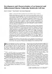
5.4.1.1.1 Simulation Results Figure 5.4.1.1 to 5.4.1.3 show the variation of e2e for as functions of various simulation parameters. Bars around each point indicate 90% confidence interval. It can be clearly seen that EAODV offers superior e2e performance compared to AODV. The reduction in mean packet latency is mainly due to the proactive behavior induced in EAODV through
41
cross-layer interactions. Note that the success of proactivity in EAODV mainly depends on the accuracy in predictions of the prediction algorithm.
As seen in Figure 5.4.1.1, EAODV offers lesser e2e delay than AODV with increase in maximum node velocity. For the same communication pattern, an increase in maximum velocity will increase the rate of change of topology, which will reduce the average lifetime of a link. This in turn will increase the number of RREQs, which will increase the control data (and hence the network traffic) transmitted. An increase in network traffic implies an increase in the rate of packets (samples) fed to the link-layer prediction algorithm, which increases the accuracy of link breakage predictions. Another fall out of the increased network control traffic (high priority) is the increased queuing delay of data (low-priority) packets. Hence, as Figure 5.4.1.1 shows, an increase in velocity will increase the e2e delay of packets.
The results from Figure 5.4.1.2 show that EAODV outperforms AODV in terms of e2e as pause time is varied. As explained earlier, the better results for e2e offered by EAODV as compared to AODV can be attributed to the proactive route discovery mechanism in EAODV, which reduces the delay of route discovery (and hence e2e) at the instant of a link breakage.
42
End-to-End delay vs max velocity (Random Waypoint Model)
0.7
0.6
e2e (seconds)
0.5
0.4
AODV EAODV
0.3
0.2
0.1
0 1
5
10
15
20
max velocity (m/s)
Figure 5.4.1.1 e2e vs Max Velocity (RW model, CBR traffic)
End-to-End delay vs pause time (Random Waypoint Model) 0.65
e2e delay (seconds)
0.6
0.55
0.5
AODV EAODV
0.45
0.4
0.35
0.3 0
250
500
1000
1500
2000
pause time (seconds)
Figure 5.4.1.2 e2e vs Pause Time (RW model, CBR traffic)
43
End-to-End delay vs mean packet interarrival time (Random Waypoint Model) 1.6
1.4
e2e (seconds)
1.2
1
AODV
0.8
EAODV 0.6
0.4
0.2
0 0.1
0.25
0.5
1
2
mean packet interarrival time (seconds)
Figure 5.4.1.3 e2e vs Mean Packet Inter-arrival time (RW model, CBR traffic)
But the surprising aspect of Figure 5.4.1.2 is the trend seen in the curves. The e2e value is lowest for a pause time of 0 seconds (which signifies least network stability), highest for a pause time of 500 seconds, and starts decreasing for higher values of pause times (or higher stability). This strange behavior could be attributed to the following reason: the degree of network partitioning in the mobility patterns chosen for the RW model is quite high because of the large simulation area chosen. Hence, higher mobility enables better connectivity. But higher mobility may be attributed to either increasing velocity or decreasing pause time.
To have a clearer picture, let us consider the curves for p.d.r (Figure 5.4.1.4 – 5.4.1.5). Though e2e may be influenced by both network traffic and delay in route discovery, p.d.r is mainly influenced by availability of routes only. Figure 5.4.1.4 shows that the p.d.r is
44
almost constant with respect to variation in velocity. But Figure 5.4.1.5 shows that for any given velocity, p.d.r decreases for increasing pause times – i.e. for any given velocity, the degree of network partitioning and probability of separation increases with increasing pause times (Table 5.4.1.1). When nodes move with higher velocities, they break and make links at a faster rate, while at slower velocities, though the rate of making links is lower, the rate of breaking links is lower as well. Hence a balance is struck between making and breaking links at all velocities. But for any given velocity, for increasing pause times, it takes longer for nodes to come closer to one another to make new links. As a result, though the average link lifetime increases (Table 5.4.1.1) due to prolonged immobility, the network remains partitioned for longer periods of time and hence the p.d.r decreases. In short, as pause-time increases, inter-partition connectivity decreases and intra-partition connectivity increases. In retrospection, it seems to be a bad idea to have chosen a mobility pattern with a high degree of network partitions, because it introduces various complexities in comparing two competing protocols. That is precisely why the simulation area for MG model was reduced (see section 5.4.1.2). In Figure 5.4.1.2, the e2e increases up to a pause time of 500 seconds and then decreases. Up to 500 seconds, the time taken to deliver a packet increases as explained above. Some packets, even if they are delayed for a long time, may be delivered eventually. But beyond 500 seconds, packets are either delivered quickly (longer link lifetimes) or are timed out and are dropped (higher network partitions). Hence the mean packet delay decreases. This argument is corroborated from the p.d.r curve (Figure 5.4.1.5), which shows p.d.r as a monotonically decreasing function of increasing pause times. Figure 5.4.1.3 is self-explanatory. As the packet interarrival time increases, queuing delay of
45
data packets decreases, and hence the trend shown in Figure 5.4.1.3. Again EAODV offers better e2e performance than AODV for the same reasons given for Figure 5.4.1.2.
As seen in Figure 5.4.1.4 and 5.4.1.5, AODV offers slightly better p.d.r performance than EAODV. This is because the prediction algorithm is not 100% accurate. It either results in proactivity too late or too soon. If proactivity is too late, then an attempt is made to route packets over a broken link, which results in packets being lost. If proactivity occurs too soon, then unwanted route discoveries are made, delaying some packets, which might get timed-out eventually. Comparing e2e and p.d.r curves for AODV and EAODV, it is clear that in EAODV, packets either get delivered quicker than AODV (if proactivity occurs at an appropriate time) or are lost (if proactivity is unwanted).
Packet Delivery Ratio vs max veloctiy (Random Waypoint Model) 1 0.95 0.9 0.85
p.d.r
0.8
AODV
0.75
EAODV 0.7 0.65 0.6 0.55 0.5 1
5
10
15
20
max velocity (m/s)
Figure 5.4.1.4 p.d.r vs Max Velocity (RW model, CBR traffic)
46
Packet Delivery Ratio vs pause time (Random Waypoint Model) 0.85
0.8
0.75
0.7
p.d.r
AODV EAODV
0.65
0.6
0.55
0.5 0
250
500
1000
1500
2000
pause time (seconds)
Figure 5.4.1.5 p.d.r vs Pause Time (RW model, CBR traffic) Packet Delivery Ratio vs mean packet interarrival time (Random Waypoint Model) 1 0.9 0.8 0.7
p.d.r
0.6
AODV
0.5
EAODV 0.4 0.3 0.2 0.1 0 0.1
0.25
0.5
1
2
mean packet interarrival time (seconds)
Figure 5.4.1.6 p.d.r vs Mean Packet Inter-arrival time (RW model, CBR traffic)
47
From Figure 5.4.1.6, it can be seen that EAODV performs almost as well as AODV in terms of p.d.r for variation in communication pattern alone. Even the e2e performance of EAODV is only marginally better than AODV for variation in communication pattern. This is because, with variation only in communication pattern, the amount of control data generated in EAODV is not much different from AODV. The ratio of control packets to data packets under frequent link breakage conditions is much higher than the same ratio under more stable conditions. As seen from Figure 5.4.1.6, we do not expect this ratio to change drastically with variation in communication pattern under similar network topological conditions, because at higher packet generation rates, the ratio of packets delivered reduces. This is mainly because of collisions in the 802.11 MAC layer at higher packet generation rates. The collisions occur because of the relatively low capacity (2 Mbps) of the wireless links and relatively bigger packet sizes (512 bytes). At higher packet generation rates, one can expect the p.d.r to improve for smaller packet sizes. As the success of the prediction algorithm (and the success of proactive route maintenance) depends mainly on the rate of both data and control packets fed to the algorithm, rate of control packets generated greatly influences the behavior of the prediction algorithm in this case. Hence, under identical network conditions, the rate of data packets generated (in our case), does not influence the behavior of the prediction algorithm in any beneficial way.
Figures 5.4.1.7 to 5.4.1.9 show the variation in c.p.d with respect to varying conditions of mobility and communication pattern. AODV seems to slightly outperform EAODV with respect to c.p.d. The increased c.p.d in EAODV can be attributed to the unwanted
48
proactive route discoveries in EAODV. As argued earlier, Figure 5.4.1.9 shows that the change in communication pattern seems to do little to separate AODV and EAODV. control bits/data bit vs max velocity (Random Waypoint Model) 0.8
0.7
ctrl bits/data bit
0.6
0.5
AODV
0.4
EAODV 0.3
0.2
0.1
0 1
5
10
15
20
max velocity (m/s)
Figure 5.4.1.7 c.p.d vs Max Velocity (RW model, CBR traffic) control bits/data bit vs pause time (Random Waypoint Model) 0.6
ctrl bits / data bit
0.5
0.4
AODV
0.3
EAODV 0.2
0.1
0 0
250
500
1000
1500
2000
pause time (seconds)
Figure 5.4.1.8 c.p.d vs Pause Time (RW model, CBR traffic)
49
control bits/data bit vs mean packet interarrival time (Random Waypoint Model) 0.9
0.8
ctrl bits/data bit
0.7
0.6
0.5
AODV EAODV
0.4
0.3
0.2
0.1
0 0.1
0.25
0.5
1
2
mean packet interarrival time (seconds)
Figure 5.4.1.9 c.p.d vs Mean Packet Inter-arrival time (RW model, CBR traffic)
For the trend of c.p.d (for both AODV & EAODV) seen in Figure 5.4.1.7, it can be intuitively argued that as the rate of topological changes increases, so will the number of control bits per data bit. Figure 5.4.1.7 seems to justify this argument. Figure 5.4.1.8 is slightly more complex - though the increase in “mobility” or increase in rate of topological changes demands more control data to be transmitted in the network, many packets in the IFQUEUE that may potentially trigger route discoveries (or control data) are lost due to time outs for lack of replies to route discoveries (due to high degree of network partitioning, as discussed for e2e). Hence the number of control packets is reduced along with the number of data packets to be transmitted. Hence the c.p.d values remain relatively unchanged with varying pause times.
50
Figure 5.4.1.9 is quite self-explanatory. For the duration of the lifetime of a route, the rate of packets delivered is higher in case of a higher source generation rate i.e. for the same amount of control data, a higher number of data packets can be delivered, which reduces c.p.d at higher generation rates. But the c.p.d and generation rate are not linearly related because, at higher generation rates, the p.d.r is lower due to collisions at the MAC layer, which serves to increase the c.p.d. For example, one might expect to see a 20-fold increase in c.p.d for an increase in mean packet inter-arrival time from 0.1 seconds to 2 seconds (20 times lesser packets generated). But as the p.d.r curves would indicate, the number of packets delivered in case of 0.1 second inter-arrival time is only about 4 times the number of packets delivered in case of a 2 second inter-arrival time; the rest of the generated packets are mostly lost through MAC layer collisions which is invisible to the AODV layer. Hence, we can expect the c.p.d to also be only approximately 4 times higher in case of a 2 second inter-arrival time when compared to the 0.1 second case, which Figure 5.4.1.9 seems to confirm as being true.
Figures 5.4.1.10 to 5.4.1.12 show the variation in the average number of hops traversed per successfully delivered packet as functions of variations in mobility and load. These figures seem to indicate that AODV offers routes with lesser number of hops to packets than EAODV. This is because AODV routes packets using the best available route (in terms of hop count) whereas EAODV routes packets using the best available route only while a reactively discovered route exists. Once the reactively discovered route breaks, the proactively discovered route is used, which may not be the best route in terms of hop count. It is important to note that in spite of the increase in hop count in EAODV, a significant reduction in end-to-end packet delay is achieved.
51
Average number of hops vs max velocity (Random Waypoint Model) 5.5
Average number of hops
5
4.5
AODV EAODV 4
3.5
3 1
5
10
15
20
max velocity (m/s)
Figure 5.4.1.10 hops vs Max Velocity (RW model, CBR traffic)
Average number of hops vs mean packet interarrival time (Random Waypoint Model) 5.5
Average number of hops
5
4.5
AODV EAODV 4
3.5
3 0.1
0.25
0.5
1
2
mean packet interarrival time (seconds)
Figure 5.4.1.12 hops vs Mean Packet Inter-arrival time (RW model, CBR traffic)
52
The trend seen in Figure 5.4.1.10 seems to indicate that in both protocols, the average number of hops is relatively immune to variation in velocity. When Figure 5.4.1.11 is studied in tandem with Figure 5.4.1.5, it is clear that at higher pause times, as a result of increased network partitioning and lesser degree of node connectivity (Table 5.4.1.1), very limited routes exist and that too with relatively higher hop counts. Figure 5.4.1.12 is consistent with our explanation so far of the effect of varying the communication pattern – at higher source rates, higher number of packets are transmitted using any existing route. But at higher source rates, the probability of packet collisions at the MAC layer increases with increasing hop count. Hence, at higher source rates, packets that use routes with lower hop-count have higher probability of getting delivered and thus we have a lower hop count at higher source rates and a relatively higher hop count at lower source rates.
Another point to note is that for e2e and hops, the confidence intervals show clear separation between EAODV and AODV curves, while for p.d.r and c.p.d, the confidence intervals of both protocols overlap. This not only strengthens the claim of relatively superior e2e performance offered by EAODV over AODV, but also slightly weakens the conclusions drawn about worse p.d.r and c.p.d performances in EAODV when compared to AODV.
5.4.1.2 Simulation parameters for Manhattan Grid Model: The simulations using MG model were run in a 1000m by 1000m area with 50 nodes under varying conditions of mobility only. The simulation area was reduced (when compared to the RW model) to reduce the average number of partitions and probability of
53
separation. We chose to conduct experiments by varying only mobility because due to the reduced simulation area, the average node degree increased (see Table 5.4.1.2) which resulted in severe MAC layer collisions at lower packet interarrival times. All statistics were based upon 40,000 data packets. Variation in mobility: The MG model has three degrees of mobility – maximum velocity, pause probability and turn probability. Our simulations were conducted by varying pause probabilities and turn probabilities. •
Pause probability varied as 0, 0.25, 0.5, 0.75, 1.0
•
Turn probability varied as 0, 0.25, 0.5, 0.75, 1.0
Maximum velocity and pause time were not varied since simulation experiments were already conducted by varying these parameters in the RW model itself. The MG model was mainly chosen because it offered additional degrees of freedom to vary mobility. The default values for pause probability and turn probability were chosen as 0 and 0.25 respectively. The maximum velocity was chosen as 10 m/s and the default pause time was 120 seconds. The communication pattern was the same default communication pattern used in the RW model. Table 5.4.1.2 gives the average values of the statistical parameters for each of the MG-mobility pattern used in the simulation experiment. It can be seen that due to increased nodal density, the partition degree and probability of separation values for MG mobility models are much lesser than corresponding values in the RW mobility models.
54
Table 5.4.1.2 Statistical Parameter values for various MG Mobility Patterns Average link Parameters Average node Average no. Probability of duration Pause Turn degree Partitions separation (seconds) Probability Probability 0
50
1
0
0.25
6.95
1.36
0.041
37.06
0.5
7.39
1.29
0.028
36.95
0.75
7.63
1.30
0.026
36.85
1.0
8.44
1.16
0.014
36.01
9.34
1.49
0.035
417.77
17.63
1.03
0.001
373.58
0.75
26.422
1
0
277.56
1.0
28.41
1
0
262.69
0
0.25 0.5 0.25
5.4.1.2.1 Simulation Results As seen from the combination of the four network statistical parameters in Table 5.4.1.2, the network is very stable for a turn probability of 0 followed by turn probabilities of 1.0, 0.75, 0.5 and 0.25 in decreasing order of stability (increasing order of mobility). From Table 5.4.1.2, it can be inferred that a pause probability of 0 represents maximum mobility, followed by pause probabilities of 0.25, 0.5, 0.75 and 1.0 in decreasing order of mobility.
55
End-to-End delay vs turn probability (Manhattan Grid Model) 0.35
0.3
e2e (seconds)
0.25
0.2
AODV EAODV
0.15
0.1
0.05
0 0
0.25
0.5
0.75
1
turn probability
Figure 5.4.1.13 e2e vs turn probability (MG model, CBR traffic)
Figure 5.4.1.13 and 5.4.1.14 show the variation of e2e as a function of turn and pause probabilities respectively. Again, it can be seen that in terms of e2e, EAODV offers mostly better or at least equal performance when compared to AODV. As explained earlier, the reduction in e2e in EAODV is mainly due to the availability of proactively discovered routes in the event of a link breakage. From Figure 5.4.1.13, it can be seen that EAODV and AODV perform alike with respect to e2e for a turn probability of 0. For other values of turn probabilities, since the network generates higher control load as a result of frequent changes in the network, EAODV offers better e2e performance than AODV.
Similarly, from Figure 5.4.1.14, it could be seen that for variation in pause probabilities, EAODV offers superior e2e performance in the maximum mobility scenario (pause
56
probability of 0), while the e2e performance of EAODV and AODV at lesser mobility scenarios becomes more or less indistinguishable. The reason is simple: higher mobility implies higher network traffic generated, which in turn improves the performance of the prediction algorithm, while lesser mobility reduces network traffic, which degrades the performance of the prediction algorithm. The e2e values increase for increasing mobility as a result of queuing delay incurred in the higher mobility cases due to increase in generation of control traffic. End-to-End delay vs pause probability (Manhattan Grid Model) 0.35
0.3
e2e (seconds)
0.25
0.2
AODV EAODV
0.15
0.1
0.05
0 0
0.25
0.5
0.75
1
pause probability
Figure 5.4.1.14 e2e vs pause probability (MG model, CBR traffic)
Figure 5.4.1.15 and 5.4.1.16 show the variation in p.d.r as a function of turn and pause probabilities respectively. As with the RW model, AODV offers slightly superior p.d.r performance than EAODV for the reasons explained while discussing p.d.r results for RW model. Also, the trend in p.d.r can be explained easily; the p.d.r drops as the number of network partitions increases (as seen from Table 5.4.1.2).
57
Packet Delivery Ratio vs turn probability (Manhattan Grid Model) 1 0.9 0.8 0.7
p.d.r
0.6
AODV
0.5
EAODV 0.4 0.3 0.2 0.1 0 0
0.25
0.5
0.75
1
turn probability
Figure 5.4.1.15 p.d.r vs turn probability (MG model, CBR traffic)
Figure 5.4.1.17 and 5.4.1.18 show the variation of c.p.d as functions of turn and pause probabilities respectively. Again, for the same reasons explained in the RW model, AODV offers slightly better c.p.d performance than EAODV. The trend seen in curves in Figure 5.4.1.17 and 5.4.1.18 can be explained as follows: the c.p.d increases with increasing degree of mobility (determined from network statistics parameters in Table 5.4.1.2) as at higher rates of mobility (less stable network conditions), more control traffic is generated to deliver comparable or lesser amount of data traffic when compared to data traffic at lesser mobility rates (see p.d.r curves).
Figure 5.4.1.19 and 5.4.1.20 show the variation of hops as a function of turn and pause probabilities respectively. Again, as with the RW mobility model, AODV supplies routes with lesser number of hops than EAODV does. The reason for this behavior has already been explained during analysis of results for hops for the RW model. The trend of curves
58
seen in Figure 5.4.1.19 and 5.4.1.20 is consistent with our explanation that the number of hops decreases as the degree of mobility of nodes in the network decreases. Packet Delivery Ratio vs pause probability (Manhattan Grid Model) 1 0.9 0.8 0.7
p.d.r
0.6
AODV
0.5
EAODV 0.4 0.3 0.2 0.1 0 0
0.25
0.5
0.75
1
pause probability
Figure 5.4.1.16 p.d.r vs pause probability (MG model, CBR traffic) control bits/data bit vs turn probability (Manhattan Grid Model) 0.9 0.8
ctrl bits/data bit
0.7 0.6 0.5
AODV EAODV
0.4 0.3 0.2 0.1 0 0
0.25
0.5
0.75
1
turn probability
Figure 5.4.1.17 c.p.d vs turn probability (MG model, CBR traffic)
59
control bits/data bit vs pause probability (Manhattan Grid Model) 0.9
0.8
ctrl bits/data bit
0.7
0.6
0.5
AODV EAODV
0.4
0.3
0.2
0.1
0 0
0.25
0.5
0.75
1
pause probability
Figure 5.4.1.18 c.p.d vs pause probability (MG model, CBR traffic)
Average num ber of hops vs turn probability (Manhattan Grid Model) 5 4.5
Average number of hops
4 3.5 3
AODV 2.5
EAODV 2 1.5 1 0.5 0 0
0.25
0.5
0.75
1
turn probability
Figure 5.4.1.19 hops vs turn probability (MG model, CBR traffic)
60
Average number of hops vs pause probability (Manhattan Grid Model) 5
Average number of hops
4.5
4
AODV
3.5
EAODV 3
2.5
2 0
0.25
0.5
0.75
1
pause probability
Figure 5.4.1.20 hops vs pause probability (MG model, CBR traffic)
From the results of simulations with RW and MG model for CBR traffic, it can be concluded that EAODV is beneficial mainly when the degree of mobility is quite high. When compared to AODV, the price paid by EAODV at higher mobility is slightly higher control overhead and slightly lesser packet delivery ratio caused due to inappropriate proactivity. EAODV does not seem to be really useful at stable network conditions, because at best, it performs only as well as AODV.
5.4.2 Simulations with TCP traffic As with CBR traffic, performances of AODV and EAODV with TCP traffic were compared across two traffic models, the Random Waypoint Model and Manhattan Grid Model. Only c.p.d, tp, e2e and hops were considered as performance metrics for TCP traffic. P.d.r was not chosen as a performance metric because TCP guarantees reliable 61
delivery and the p.d.r values were expected to be indistinguishable for TCP over AODV and EAODV.
5.4.2.1 Simulations with Random Waypoint Model The simulations using RW model were run in a 1500m by 1500m area with 50 nodes under varying conditions of mobility only. The communication model consisted of 20 TCP connections, with a packet size of 512 bytes for each set of simulations. Each connection was simulated as a FTP transfer of a very large file, so that TCP traffic was continuously generated through out the entire duration of simulation. TCP-Tahoe was the flavor of TCP used. All statistics were based upon data packets collected over 1000 simulation seconds. Variation in mobility: The RW model has two degrees of mobility – maximum velocity and pause time. Our simulations were conducted by varying both maximum velocity and pause time. •
Maximum velocity varied as 1, 5, 10, 15, 20 m/s
•
Pause time varied as 0, 250, 500, 750, 1000 seconds
For the RW mobility model, the default values for maximum velocity and pause time were 10 m/s and 0 seconds respectively. Note that the mobility scenario files used for TCP simulations and CBR simulations were the same.
5.4.2.1.1 Simulation Results Figures 5.4.2.1 and 5.4.2.2 show the variation of c.p.d with respect to variation in maximum velocity and pause time respectively. As seen from these plots, it is clear that EAODV offers superior c.p.d performance compared to AODV. The reason for decrease
62
in c.p.d in EAODV can be attributed to the excellent performance of the prediction algorithm. With TCP traffic, the number of MAC frames carrying IP-encapsulated TCP segments is comparable to the number of control packets generated, and hence the prediction algorithm has the luxury of predicting link breakage time with the help of a large number of packets. As a result, with EAODV, the number of link breaks in active routes is reduced (by effective preemptive switching of active routes) when compared to the number of link breaks in AODV, which reduces the control traffic generated. Figures 5.4.2.3 and 5.4.2.4 show the variation of TCP throughput as functions of maximum velocity and pause time respectively. These curves indicate that the throughputs achieved in EAODV and AODV are nearly the same. Hence, under conditions of comparable throughput, EAODV offers lesser c.p.d than AODV.
The trend seen in the Figures 5.4.2.1 can be explained as follows: higher velocity implies higher mobility, which not only increases the network traffic generated, but also decreases the throughput values (Figure 5.4.2.3). The net result of these effects is the increase in c.p.d for increasing velocities. To explain the trend in Figure 5.4.2.2, consider the following: it can be seen from Table 5.4.1.1 that higher values of pause times represent lesser mobility and longer link lifetimes. Lesser mobility and longer link lifetimes enable that TCP connection to generate bursts at a higher rate for a longer duration. But at higher pause time values, the degree of network partition also increases. As a result, in some connections that have the sources and destinations in different partitions, there are frequent TCP retransmissions. These retransmissions reduce the source TCP’s window size to the minimum value, and packets are generated at a very
63
slow rate until the partitions merge. Since TCP packets in such connections are generated at a very low rate, the rate of control traffic generated is also very small for the duration of the partition (Please remember that RREQs are generated only when there are outstanding packets in the AODV queue for a particular destination). Also, as seen from Figure 5.4.2.4, the throughput at higher pause times tends to be higher, which further decreases the control traffic to data traffic ratio. Hence, the c.p.d decreases for increasing pause times.
The reason for the trend seen in Figure 5.4.2.3 is simple: higher velocity implies higher mobility, and frequent link breaks. These link breaks reduce the average window size of TCP, which reduces the throughput. Thus at higher velocities, throughput is reduced. As seen from Figure 5.4.2.4, the throughput tends to be higher at higher pause times. At higher pause times, though the degree of partition is higher, the higher throughput achieved in connections that span stable links offsets the lower throughput in “connections” spanning partitions, whereas at lower pause times, the increased mobility of nodes reduces the throughput. This explains the trend in the throughput curves.
Figures 5.4.2.5 and 5.4.2.6 show the variation of e2e as a function of maximum velocity and pause time. The separation between e2e performances in EAODV and AODV is quite unclear because the confidence intervals overlap, although from the curves, one can conclude with lesser confidence that EAODV gives better e2e performance than AODV. Figure 5.4.2.5 shows that e2e decreases with increasing velocities. This is because with increasing velocities, routes are broken quickly and also made quickly, while at lower velocities, routes are broken slowly and also made slowly. At lower velocities, once the
64
route is broken, retransmissions may occur because the delay in forming a new route is higher. The decrease in delay due to higher rate of bursts possible at lower velocities is offset by the increase in delay due to retransmissions as a result of broken links and increase in queuing delay due to congestion (and possible retransmission) at higher source rates. The effect of increased queuing delay due to increased network traffic due to numerous route discoveries at higher velocities is lesser than the effect of increased delay due to congestions and retransmissions in the lower velocity case, and hence e2e decreases with increasing velocities. As shown in Figure 5.4.2.6, e2e first decreases with increasing pause times, since increasing pause times represent decreasing mobility. But beyond a pause time of 500 seconds, the e2e starts increasing because the decrease in delay due to decreased mobility is offset by an increase in delay due to retransmissions, which is more pronounced when the network is highly partitioned. control bits/ data bit vs max velocity (Random Waypoint Model) 0.045
0.04
ctrl bits/data bit
0.035
0.03
0.025
AODV EAODV
0.02
0.015
0.01
0.005
0 1
5
10
15
20
max velocity (m/s)
Figure 5.4.2.1 c.p.d vs Max Velocity (RW model, TCP traffic)
65
control bits/ data bit vs pause time (Random Waypoint Model) 0.035
0.03
ctrl bits/data bit
0.025
0.02
AODV EAODV
0.015
0.01
0.005
0 0
250
500
750
1000
pause time (seconds)
Figure 5.4.2.2 c.p.d vs Pause time (RW model, TCP traffic) Throughput vs max velocity (Random Waypoint Model)
0.7
Throughput (Mbps)
0.6
0.5
0.4
AODV EAODV
0.3
0.2
0.1
0 1
5
10
15
20
max velocity (m/s)
Figure 5.4.2.3 Throughput vs Max Velocity (RW model, TCP traffic)
66
Throughput vs pause time (Random Waypoint Model) 0.7
Throughput (Mbps)
0.6
0.5
0.4
AODV EAODV
0.3
0.2
0.1
0 0
250
500
750
1000
pause time (seconds)
Figure 5.4.2.4 Throughput vs Pause time (RW model, TCP traffic)
End-to-End delay vs m ax velocity (Random Waypoint Model) 0.34
e2e delay (seconds)
0.32
0.3
0.28
AODV EAODV
0.26
0.24
0.22
0.2 1
5
10
15
20
m ax velocity (m /s)
Figure 5.4.2.5 e2e vs Max Velocity (RW model, TCP traffic)
67
End-to-End delay vs pause time (Random Waypoint Model) 0.3
e2e delay (seconds)
0.25
0.2
AODV
0.15
EAODV 0.1
0.05
0 0
250
500
750
1000
pause time (seconds)
Figure 5.4.2.6 e2e vs Pause time (RW model, TCP traffic)
Average number of hops vs max velocity (Random Waypoint Model) 3
Average number of hops
2.5
2
AODV
1.5
EAODV 1
0.5
0 1
5
10
15
20
max velocity (m/s)
Figure 5.4.2.7 hops vs Max Velocity (RW model, TCP traffic)
68
Average number of hops vs pause time (Random Waypoint Model) 3
Average number of hops
2.5
2
AODV
1.5
EAODV 1
0.5
0 0
250
500
750
1000
pause time (seconds)
Figure 5.4.2.8 hops vs Pause time (RW model, TCP traffic)
As seen from Figures 5.4.2.7 and 5.4.2.8, the average number of hops traversed per delivered packet in both AODV and EAODV is almost the same. Moreover, the number of hops seems relatively oblivious to the variation in maximum velocity or pause time. Please keep in mind that the hop count obtained with CBR traffic is a true measure of the average hop count of all active routes in the simulation, as the traffic source is independent of the network condition, while the hop count obtained with TCP traffic is not. This is because, in the absence of congestion, the rate of TCP transmissions is very sensitive to the number of hops, because the rate depends on the mean round trip time (rtt) of each connection, which is largely dependant on the number of hops. Hence at lower hop counts, TCP transmits at a very high rate, while the rate rapidly drops at higher hop counts. Thus, the average hop count in TCP tends to be similar for all simulations just as the average hop count across all CBR simulations are comparable. Since TCP
69
operates as a feedback system, TCP has a lower average hop count than the average hop count with CBR traffic for the same mobility scenario.
5.4.2.2 Simulation parameters for Manhattan Grid Model: The simulations using MG model were run in a 1000m by 1000m area with 50 nodes under varying conditions of mobility only. All statistics were based upon data packets collected over 1000 simulation seconds Variation in mobility: The MG model has three degrees of mobility – maximum velocity, pause probability and turn probability. Our simulations were conducted by varying pause probabilities and turn probabilities. •
Pause probability varied as 0, 0.25, 0.5, 0.75, 1.0
•
Turn probability varied as 0, 0.25, 0.5, 0.75, 1.0
The default values for pause probability and turn probability were chosen as 0 and 0.25 respectively. The maximum velocity was chosen as 10 m/s and the default pause time was 120 seconds. The communication pattern was the same communication pattern used in the RW model.
5.4.2.2.1 Simulation Results Figures 5.4.2.9 and 5.4.2.10 show the variation of c.p.d as functions of turn and pause probabilities respectively, while Figures 5.4.2.11 and 5.4.2.12 plot the variation of TCP throughput as functions of turn and pause probabilities respectively. Figures 5.4.2.13 and 5.4.2.14 depict the variation of e2e with variations in turn and pause probabilities respectively, while Figures 5.4.2.15 and 5.4.2.16 show the variation of average number of hops as functions of turn and pause probabilities respectively.
70
From Figures 5.4.2.9 and 5.4.2.10, it can be seen that EAODV seems to offer better c.p.d performance than AODV in most cases. For variation in turn probability, the effect of reduction in number of link breaks (and subsequent reduction in control traffic generated) on c.p.d in EAODV offsets the effect of reduced throughput (Figure 5.4.2.11) on c.p.d due to EAODV using routes with higher hop counts than AODV, resulting in lesser c.p.d in EAODV than in AODV. The trend seen in c.p.d for varying values of turn probabilities is quite similar to the trend seen with CBR traffic. For variation in pause probability, the c.p.d in EAODV decreases when compared to AODV, as the reduction in number of link breaks in EAODV reduces the control data generated for comparable throughputs in EAODV and AODV (Figure 5.4.2.12). The trend seen in Figure 5.4.2.10 is consistent with our earlier explanation for reduction in c.p.d for increasing pause probabilities.
As seen from Figures 5.4.2.13 - 5.4.2.14 and Figures 5.4.2.15 – 5.4.2.16, the e2e and average number of hop behavior of both EAODV and AODV are almost indistinguishable. The e2e values are almost the same in both EAODV and AODV because only a small fraction of packets out of the total delivered packets in EAODV benefit from the reduction in delay due to proactive route discovery, and hence their effect on the resultant e2e value is negligible. The trends as seen in Figures 5.4.2.11 – 5.4.2.16 are quite surprising. In all of these curves, for the simulation parameters corresponding to the most stable network, throughput and e2e exhibit worst performance, while the hops corresponding to these parameters exhibit best performance.
71
In these cases of maximum network stability, though control traffic is greatly reduced, the average number of neighboring nodes is very high (Table 5.4.1.2). This increases the degree of contention in the wireless physical channel because the simulation model uses only a single channel (frequency) for communication between nodes. This in turn increases the probability of collision of the control (RTS/CTS/ACK) packets at the MAC 802.11 (CSMA/CA) layer. Hence, higher the average node degree, higher is the collision probability. The collisions require the transmitting nodes to perform an exponential backoff, which greatly reduces link utilization and effective bandwidth. Hence, in such highly inter-connected networks, the e2e and tp performances experience degradation.
control bits/ data bit vs turn probability (Manhattan Grid Model) 0.1 0.09 0.08
ctrl bits/data bit
0.07 0.06
AODV
0.05
EAODV 0.04 0.03 0.02 0.01 0 0
0.25
0.5
0.75
1
turn probability
Figure 5.4.2.9 c.p.d vs turn probability (MG model, TCP traffic)
72
control bits/ data bit vs pause probability (Manhattan Grid Model) 0.05 0.045 0.04
ctrl bits/data bit
0.035 0.03
AODV
0.025
EAODV 0.02 0.015 0.01 0.005 0 0
0.25
0.5
0.75
1
pause probability
Figure 5.4.2.10 c.p.d vs pause probability (MG model, TCP traffic)
Throughput vs turn probability (Manhattan Grid Model) 0.6
Throughput (Mbps)
0.5
0.4
AODV
0.3
EAODV 0.2
0.1
0 0
0.25
0.5
0.75
1
turn probability
Figure 5.4.2.11 Throughput vs turn probability (MG model, TCP traffic)
73
Throughput vs pause probability (Manhattan Grid Model) 0.7
Throughput (Mbps)
0.6
0.5
0.4
AODV EAODV
0.3
0.2
0.1
0 0
0.25
0.5
0.75
1
pause probability
Figure 5.4.2.12 Throughput vs pause probability (MG model, TCP traffic)
End-to-End Delay vs turn probability (Manhattan Grid Model) 2.2 2
e2e delay (seconds)
1.8 1.6 1.4
AODV
1.2
EAODV 1 0.8 0.6 0.4 0.2 0
0.25
0.5
0.75
1
turn probability
Figure 5.4.2.13 e2e vs turn probability (MG model, TCP traffic)
74
End-to-End Delay vs pause probability 2.2 2
e2e delay (seconds)
1.8 1.6 1.4
AODV
1.2
EAODV 1 0.8 0.6 0.4 0.2 0
0.25
0.5
0.75
1
pause probability
Figure 5.4.2.14 e2e vs pause probability (MG model, TCP traffic)
Average number of hops vs turn probability (Manhattan Grid Model) 3
Average number of hops
2.5
2
AODV
1.5
EAODV 1
0.5
0 0
0.25
0.5
0.75
1
turn probability
Figure 5.4.2.15 hops vs turn probability (MG model, TCP traffic)
75
Average num ber of hops vs pause probability (Manhattan Grid Model) 3
Average number of hops
2.5
2
AODV 1.5
EAODV 1
0.5
0 0
0.25
0.5
0.75
1
pause probability
Figure 5.4.2.16 hops vs pause probability (MG model, TCP traffic)
From the simulation results with TCP traffic, it can be concluded that: •
EAODV offers slightly better c.p.d performance than AODV in most cases
•
EAODV offers slightly better e2e performance than AODV in networks that are not very stable; the e2e in EAODV is almost indistinguishable from e2e in AODV for stable networks
•
EAODV offers comparable throughput performance with AODV in most cases
•
The hops in both AODV and EAODV are comparable in most cases.
•
In both EAODV and AODV, the network experiences maximum congestion when the network is most stable. The congestion can be alleviated if link rates are increased.
76
5.4.3 Comparison of CBR and TCP results A comparison of CBR and TCP simulation results yields interesting conclusions. The c.p.d in case of TCP is much lesser than the c.p.d in CBR. The reasons are two-fold: (1) In the absence of congestion, TCP generates maximum traffic over stable links, and reduces traffic burst rate over less stable links, while CBR generates traffic independent of the state of the links, thus increasing the control traffic overhead (2) Since c.p.d is calculated over the number of packets delivered, TCP has lesser c.p.d than CBR – TCP guarantees reliable delivery, while CBR is unreliable delivery and hence in CBR the fraction of packets delivered is almost always lesser than in TCP. For identical mobility scenarios, TCP has lesser e2e than UDP. The rate control mechanism in TCP-Tahoe forces TCP to generate higher rates of bursty traffic when the average rtt is lower, thus generating a large number of packets at very low end-to-end delay and very less packets at higher end-to-end delay, which leads to lower e2e value. CBR, on the other hand, does not have any rate control mechanism, and hence generates packets evenly under all conditions and has a higher e2e value.
The most interesting observation is the hops behavior in both TCP and CBR traffic. As explained earlier, due to the rate limiting property of TCP-Tahoe, TCP generates higher rates of bursts when the hop count is lesser and at lesser rates of bursts at higher hop counts, while CBR, as explained above, has no feedback mechanism, and always generates packets at an even rate (evidence for this claim is presented in Figures 5.4.3.1 and 5.4.3.2, and discussed later). In the absence of congestion, the rtt increases linearly with the number of hops. This leads to an overall smaller hop count. The fallout of this
77
rate limiting property in TCP is that whenever a link breaks, the delay experienced by a TCP packet for route discovery before delivery will increase the rtt of the connection (and maybe cause some timeouts and retransmissions). TCP misinterprets this increase in rtt (and retransmissions) as congestion, and multiplicatively decreases its window size. Even if the rtt value falls subsequently, the window size is only increased additively. This behavior can cause potential damage to TCP throughput. If TCP can distinguish between increase in rtt due to link breakage and real network congestion, and act accordingly, the throughput can be increased. Even if TCP is enabled to distinguish between reasons for increase in rtt, TCP still needs reduction in window size during link breakages, because link breakages can cause queue build-up at the various nodes, and if TCP continues to transmit at the same rate, there is scope for congestion to occur. TCP can additively decrease window size during times of link breakage, and multiplicatively decrease during congestion, to improve throughput.
Figures 5.4.3.1 and 5.4.3.2 show the number of TCP and CBR packets received by a tagged node at each instant of time (with a one second granularity) for each hop count value under identical mobility conditions. The simulations were run separately for default TCP and CBR communication patterns using the AODV protocol with the same mobility pattern file. The mobility pattern was chosen to represent maximum mobility (RW model, maximum velocity of 20 m/s and pause time of 0 second), so that the behavior of the transport layer protocols (read UDP and TCP) is best studied under extremely transient network conditions. Also, the number of received packets in the tagged node is monitored
78
(instead of the generated packets) because the received packets best characterize the overall behavior of the various sources for varying network conditions. Number of TCP packets received (tagged node)vs time 140
Number of packets received
120
1 2
100
3 4
80
5 6 60
7 8
40
9 10
20
0 0
80
160
240
320
400
480
560
640
720
800
880
960
time (seconds)
Figure 5.4.3.1 Number of TCP packets vs Time Num ber of CBR packets received (tagged node)vs tim e 18
16
Number of packets received
1 14
2 3
12
4 10
5 6
8
7 6
8 9
4
10 2
0 0
80
160
240
320
400
480
560
640
720
800
tim e (seconds)
Figure 5.4.3.2 Number of CBR packets vs Time
79
880
960
In Figures 5.4.3.1 and 5.4.3.2, each entry in the legend is the hop count value. Comparing Figures 5.4.3.1 and 5.4.3.2, TCP generates high rates of bursts at smaller hop counts, and smaller rates of bursts at higher hop counts. The sizes of the bursts in TCP have a correlation with the hop count.
5.5 Conclusions From the simulations conducted, the following conclusions can be drawn: •
For CBR traffic, EAODV is more beneficial at higher mobility scenarios
•
For TCP traffic, EAODV performs slightly better than AODV in most cases
•
For TCP traffic, in both EAODV and AODV, the network experiences maximum congestion when the average node degree is the highest.
•
For TCP running over Ad hoc networks, slight modifications in TCP may be required to increase TCP throughput
80
Chapter 6 Conclusions and Future work
This chapter summarizes the total research work done so far and the conclusions drawn from the results obtained. We also briefly discuss the potential for future research work.
6.1 Summary of work done •
Developed a prediction algorithm to predict link breakage time from signal strength information extracted from a packet received on that particular logical link
•
Implemented the prediction algorithm in the ns-2 simulator at the 802.11 wireless MAC layer
•
Derived EAODV from AODV by suitably modifying AODV to enable crosslayer interactions with the MAC layer
•
Characterized the behavior of EAODV with CBR traffic, and compared performances of EAODV and AODV with CBR traffic sources
•
Characterized behavior of EAODV with TCP traffic, and compared performances of EAODV and AODV with TCP traffic sources
6.2 Conclusions From the results of simulation experiments, the following conclusions can be drawn: •
For CBR traffic, EAODV is more beneficial at higher mobility scenarios. In higher mobility scenarios, EAODV experiences a slightly higher control overhead and slightly lesser packet delivery ratio than AODV. But the improvement in
81
mean packet end-to-end delay in EAODV outweighs the potential disadvantages of using EAODV. •
For TCP traffic, EAODV performs slightly better than AODV in most cases. EAODV always seems to offer slightly better performance in terms of end-to-end packet delay and control overhead when compared to AODV. In some cases, the throughput of EAODV slightly drops when compared to AODV. Overall, when compared to AODV, EAODV does not offer any significant benefits for TCP traffic
•
For TCP traffic, in both EAODV and AODV, the network seems to experience maximum congestion when the network is most stable.
•
For TCP running over Ad hoc networks, slight modifications in TCP may be required to increase TCP throughput. The above observations about TCP performance highlight the need for cross-layer interaction schemes in ad hoc routing.
6.3 Future Work •
One avenue for future research is to test EAODV by introducing effects of fading in the ns2 packet corruption model, which will test the prediction algorithm more rigorously for the effects of transients.
•
The suitability of EAODV for real-time traffic needs to be further studied by testing it with smaller sized CBR packets at a higher packet rate.
•
The behavior of TCP over ad hoc network routing protocols should be an area of interesting research. From the results of the simulations, it can be seen that TCP exhibits several intriguing properties over ad hoc networks. The reasons for these 82
behaviors are not fully explained. Further research is required to understand fully TCP’s behavior over ad hoc networks. •
The need to shield TCP from effects of rapidly changing network topologies is definitely felt at this point. One way of achieving this is through cross-layer interactions between various protocol layers. Further study in this direction will be very useful.
83
References [1] Joseph Macker and Scott Corson, IETF Mobile Ad Hoc Networks (MANET) Charter, http://www.ietf.org/html.charters/manet-charter.html. [2] Charles E. Perkins, Pravin Bhagwat, “Highly Dynamic Destination-Sequenced Distance-Vector Routing (DSDV) for Mobile Computers.” Proceedings of the Conference on Communications Architectures, Protocols and Applications, pages 234244, London, England, August 1994. [3] T. Clausen, P. Jacquet, A. Laouiti, P. Muhlethaler, a. Qayyum et L. Viennot “Optimized Link State Routing Protocol”, IEEE INMIC Pakistan 2001. [4] Johnson, D. and Maltz, D. (1996). "Dynamic source routing in ad hoc wireless networks," in Mobile Computing (ed.T. Imielinski and H. Korth), Kluwer Academic Publishers, Dordrecht, The Netherlands. [5] C.Perkins, E.Royer and S.Das “Ad hoc On-Demand Distance Vector (AODV) Routing”, Mobile Ad Hoc Networking Working Group, IETF Internet Draft, June 2002 http://www.ietf.org/internet-drafts/draft-ietf-manet-aodv-12.txt [6] Z.J. Haas and M.R. Pearlman, "The Zone Routing Protocol (ZRP) for Ad Hoc Networks," Internet Draft, draft-ietf-manet-zone-zrp-02.txt, June 1999 [7] Qin, L., “Pro-active Route Maintenance in DSR”, M. Sc. Thesis, School of Computer Science, Carleton University, August 2001. [8] David A. Maltz, Josh Broch, Jorjeta Jetcheva and David B. Johnson, “The Effects of On-Demand Behavior in Routing Protocols for Multihop Wireless Ad Hoc Networks”, IEEE Journal on Selected Areas in Communications Special Issue on Mobile and Wireless Networks, pages 1439-1453, August 1999.
84
[9] Vincent D. Park and M. Scott Corson, “A Performance Comparison of the Temporally-Ordered Routing Algorithm and Ideal Link-State Routing”, Proceedings of IEEE Symposium on Computers and Communication ‘98, pages 592-598, Athens, Greece, June 1998. [10] SSA: R. Dube, C.D. Rais, K.-Y. Wang, and S.K. Tripathi, “Signal Stability-Based Adaptive
Routing
(SSA)
for
Ad
Hoc
Mobile
Networks”,
IEEE
Personal
Communications, vol. 4, no. 1, Feb. 1997, pp. 36-45. [11] Elizabeth M. Royer and C.-K. Toh, “A Review of Current Routing Protocols for AdHoc Mobile Wireless Networks”, IEEE Personal Communications Magazine, pages 4655, April 1999. [12] Samir R. Das, Charles E. Perkins and Elizabeth M. Royer, “Performance Comparison of Two On-demand Routing Protocols for Ad Hoc Networks”, Proceedings of the IEEE Conference on Computer Communications, pages 3-12, Tel Aviv, Israel, March 2000. [13] Josh Broch, David A. Maltz, David B. Johnson, Yih-Chun Hu and Jorjeta Jetcheva, “A Performance Comparison of Multi-Hop Wireless Ad Hoc Network Routing Protocols”, Proceedings of the Fourth Annual ACM/IEEE International Conference on Mobile Computing and Networking, pages 85-97, Dallas, TX, October 1998. [14] Daehyoung Hong and Stephen Rappaport, “Traffic Models and Performance Analysis for Cellular Mobile Radio Telephone Systems with Prioritized and NonPrioritized Handoff Procedures”, IEEE Transactions on Vehicular Technology, Vol. VT35, No.3, pages 77-92, August 1986.
85
[15] He Dajing, Jiang Shengming and Rao Jianqiang, “A Link Availability Prediction Model for Wireless Ad Hoc Networks”, Proceedings of the International Workshop on Wireless Networks and Mobile Computing, D7-D11, Taipei, Taiwan, April 2000. [16] B. Narendran, P. Agrawal and D. K. Anvekar, “Minimizing Cellular Handover Failures
without
Channel
Utilization
Loss”,
Proceedings
of
IEEE
Global
Communications Conference, pages 1679-1685, vol. 3, December 1994. [17] The Network Simulator - ns-2 http://www.isi.edu/nsnam/ns/ [18] Kevin Fall and Kannan Varahan, editors. NS Notes and Documentation. The VINT Project, UC Berkeley, LBL, USC/ISI, and Xerox PARC, November 1997. [19] Bruce Tuch, “Development of WaveLAN, an ISM Band Wireless LAN”, AT&T Technical Journal, 72(4), pages 27-33, July/August 1993. [20] “Selection Procedures for the Choice of Radio Transmission
Technologies
of the UMTS” (TS30.03 v3.2.0). TS 30.03 3GPP, April 1998. [21] C.D. Waal “BonnMotion - a mobility scenario generation and analysis tool”, Institute
of
Computer
Science
IV,
University
bonn.de/IV/BonnMotion/
86
of
Bonn
http://www.cs.uni-
Appendix In this appendix, the codes added to the appropriate files in the ns-2 simulator software are listed (along with the file names).
node.h #define CROSS_LAYER
#ifdef CROSS_LAYER #define V_MAX 40.0 //maximum velocity of the nodes #define V_MIN 1.0 //minimum velocity of nodes #define D_MAX 250.0 // transmission range in meters #define CONSTANT 1.5 //grouping remaining terms in two-ray propogation model #define CURRENT_TIME Scheduler::instance().clock() #define MAX_TIME 50.0 //max time of consideration of the state of a link in seconds #define IDLE_TIME 15.0 //max time elapsed after which link is considered idle #define T_DEV_MAX 4.0 //max permissible deviation in time interval between samples #define V_DEV_MAX 2.0 //max permissible deviation in velocity #define MIN_SAMPLES 4 //minimum number of samples to base our estimation upon #define MaX(a,b) ((a) > (b) ? (a) : (b)) #define MiN(a,b) ((a) < (b) ? (a) : (b)) class linklifeEntry { public: enum linkstatus //enum to hold state of link enum movement {INWARD,STATIC,OUTWARD}; movement
//
{ACTIVE_LINK,IDLE_LINK,USELESS_LINK}; //enum for direction of
linklifeEntry(); linklifeEntry(u_int32_t,u_int32_t); link_life_entry(u_char); ~linklifeEntry(){;}
u_int32_t get_da() {return da;} //return destination mac address double get_expire_time() {return expire_time;} //return expire time of link double get_timestamp() {return timestamp;} //return timestamp of last updation double get_active_timestamp() {return active_timestamp;} //return active timestamp nsaddr_t getid() {return id;} //get destination node address linkstatus get_link_status() { return status;} //return link status movement get_direction(){ return direction;} //get the direction in which the node is moving bool get_status_flag(){return status_flag;} //get status_flag void update_expire_time(Packet *); //compute expire time from algorithm void update_link_status(); //update the status of the link void update_direction(); //update direction of movement void reset_df(); //reset all direction counters int mac_compare(u_int32_t);
87
int id_compare(nsaddr_t); void set_status_flag(bool stat_flag) {status_flag = stat_flag;} void reset_algorithm(); void dump(); //dump all important values to screen // void set_max_velo(double mv){maxvelo_ = mv;} // set max velocity from tcl script LIST_ENTRY(linklifeEntry) lle_link;
private: u_int32_t u_int32_t nsaddr_t int indicating direction changes!! int double link will break double bool
da; sa; id;
//other node's mac address //this node's mac address //forwarding node's ip address (id) direction_flag[3];
//# of samples
no_samples; expire_time;
//no of samples // predicted time when
timestamp;
// time of updation
status_flag;
//flag to set status as
active double
active_timestamp;
//timestamp when link was
double
v;
//instantaneous estimated
last active
velocity double
V_avg;
//estimated averaged
velocity double
d;
//estimated distance from
current node double d_prev; distance from current node double alpha; double t_break; lifetime double t_break_prev; t_break double T_avg; sampling intervals double num; squared error double denom; squared error double nmse; linkstatus status; movement direction; // double maxvelo_; /* * Now the predictor function * */ double residual_life_time(); }; LIST_HEAD(rll_table,linklifeEntry); #endif //CROSS_LAYER
node.cc Node::~Node()
88
//estimated previous //confidence index //estimate residual link//last known value of //weighted average of //numerator of mean //denominator of mean //nmse value //status of link //direction of movement
{ #ifdef CROSS_LAYER linklifeEntry *lle ; while((lle = rll_head.lh_first)){ LIST_REMOVE(lle,lle_link); delete lle; } #endif LIST_REMOVE(this, entry); } #ifdef CROSS_LAYER void linklifeEntry::reset_algorithm(){ expire_time timestamp
= 0.0; = 0.0;
active_timestamp status_flag v V_avg d d_prev alpha t_break T_avg direction status t_break_prev no_samples reset_df();
= = = = = = = = = = = = =
CURRENT_TIME; true; V_MIN; V_MIN; 0.0; D_MAX; 0.0; 0.0; 0.0; INWARD; USELESS_LINK; 0.0; 0;
} linklifeEntry::linklifeEntry(){ reset_algorithm(); num = 0.0; denom = 1.0; nmse = 0.0; } linklifeEntry::linklifeEntry(u_int32_t my_addy,u_int32_t addy){ sa = my_addy; da = addy; reset_algorithm(); num = 0.0; denom = 1.0; nmse = 0.0; }
void linklifeEntry::update_expire_time(Packet *p){ Node *node = (Node*)(p->txinfo_.getNode()); id= node->nodeid(); //update forwarding node id, incase the ip address changes, while mac remains the same!! d = pow((p->txinfo_.getTxPr()/p->txinfo_.RxPr),0.25) * CONSTANT; //estimate distance if(status_flag == true){ no_samples++; active_timestamp = CURRENT_TIME; } expire_time = CURRENT_TIME + residual_life_time(); // set expiration time } double linklifeEntry::residual_life_time(){ float epsilon = 0.01;
89
double delta_T = 0.0 ,t_wt = 1.0, v_wt = 1.0,t_ratio,v_ratio; // Calculate T_avg if(timestamp == 0.0){ //first sample timestamp = CURRENT_TIME; }
delta_T = CURRENT_TIME - timestamp;
//calculate delta_T
if(T_avg == 0.0) or algorithm reset T_avg = delta_T;
//first sample
if(delta_T > 0.0){ v = fabs( (d - d_prev)/(delta_T) );
assert(T_avg > 0.0);
//Make sure no division by zero
t_ratio = delta_T/T_avg;
//get a positive value for ratio
t_ratio = t_ratio > 1.0 ? t_ratio : (1.0/t_ratio);
//normalize ratio to >
1 t_ratio = t_ratio < T_DEV_MAX ? t_ratio : T_DEV_MAX; max t_ratio to max deviation allowed in 't' t_wt = t_ratio/T_DEV_MAX; t_wt from (1/max_dev) to 1
if(V_avg > 0.0) v_ratio = v/V_avg;
//limit //find
//find deviation of v from V_avg
v_ratio = v_ratio > 1.0 ? v_ratio : (1.0/v_ratio);
//normalize ratio to
> 1 v_ratio = v_ratio < V_DEV_MAX ? v_ratio : V_DEV_MAX; //limit max v_ratio to max deviation allowed in v v_wt = t_wt * (v_ratio/V_DEV_MAX); //find v_wt!! } /////////////////////////////////////////////////////////////////////////////////// //MAIN PART OF THE ALGORITHM ////////////////////////////////////////////////////////////////////////////////// T_avg = t_wt * delta_T + (1 - t_wt) * T_avg; //calculate T_avg T_avg = T_avg < MAX_TIME ? T_avg : MAX_TIME; //limit maximum average time to TIME_USELESS V_avg = v_wt * v + (1 - v_wt) * V_avg; V_avg = V_avg < maxvelo_ ? V_avg : maxvelo_; velocity to V_MAX
//calculate V_avg //limit maximum
///////////////////////////////////////////////////////////////////////////////////////// //////////////////////////////////////////////////////////////////////////////////////// t_break_prev = t_break; if (V_avg > 0.0){ t_break = (D_MAX - d)/V_avg; //calculate t_break t_break = t_break < MAX_TIME ? t_break : MAX_TIME; //fix upper limit on t_break } else t_break = MAX_TIME; the link if (denom > 0.0) if (nmse != num/denom){ nmse = num/denom; dump();
//set max time of interest in the state of
90
}
//set direction of movement of mobile node if(d > d_prev) direction_flag[OUTWARD]++; else if(d < d_prev) direction_flag[INWARD]++; else if (d == d_prev) direction_flag[STATIC]++; d_prev = d; timestamp = CURRENT_TIME; return t_break; };
int linklifeEntry::mac_compare(u_int32_t addy){ if(addy != da) return 0; return 1; } void linklifeEntry::dump(){ // %f
printf("\n %f: src = %u dst = %u d = %f d_prev = %f v = %f V_avg = %f t_break = dir=%d link=%d",CURRENT_TIME,sa,da,d,d_prev,v,V_avg,t_break,direction,status); if(sa == 18) coutget_expire_time() < now)) { #else if ((rt->rt_flags == RTF_UP) && (rt->rt_expire < now)) { #endif ------------------------------------------------------#ifdef CROSS_LAYER else if (rt->rt_flags == RTF_UP || rt->rt_flags == RTF_PA_REPAIR) { #else else if (rt->rt_flags == RTF_UP) { #endif // If the route is not expired, // and there are packets in the sendbuffer waiting, // forward them. This should not be needed, but this extra // check does no harm. assert(rt->rt_hops != INFINITY2); while((p = rqueue.deque(rt->rt_dst))) { forward (rt, p, delay); delay += ARP_DELAY; } } else if (rqueue.find(rt->rt_dst)) // If the route is down and // if there is a packet for this destination waiting in // the sendbuffer, then send out route request. sendRequest // will check whether it is time to really send out request // or not. // This may not be crucial to do it here, as each generated // packet will do a sendRequest anyway. sendRequest(rt->rt_dst); } ----------------------------}
void AODV::recvRequest(Packet *p) {
96
struct hdr_ip *ih = HDR_IP(p); struct hdr_aodv_request *rq = HDR_AODV_REQUEST(p); aodv_rt_entry *rt; /* * Drop if: * - I'm the source * - I recently heard this request. */
------------------------------------------------------------/* Find out whether any buffered packet can benefit from the #ifdef CROSS_LAYER if (rt0 && (rt0->rt_flags == RTF_UP || rt0->rt_flags == RTF_PA_REPAIR)) { #else if (rt0 && (rt0->rt_flags == RTF_UP)) { #endif assert(rt0->rt_hops != INFINITY2); forward(rt0, buffered_pkt, NO_DELAY); } } } // End for putting reverse route in rt table ---------------------------------------------------------------forward((aodv_rt_entry*) 0, p, DELAY); } } void AODV::forward(aodv_rt_entry *rt, Packet *p, double delay) { struct hdr_cmn *ch = HDR_CMN(p); struct hdr_ip *ih = HDR_IP(p); if(ih->ttl_ == 0) { #ifdef DEBUG fprintf(stderr, "%s: calling drop()\n", __PRETTY_FUNCTION__); #endif // DEBUG drop(p, DROP_RTR_TTL); return; } if (rt) { #ifdef CROSS_LAYER traffic_history * th = rt->th_lookup(ih->saddr()); if(!th) th = rt->th_add(ih->saddr()); double t_elapsed = CURRENT_TIME - th->th_timestamp; if(t_elapsed > 4 * th->th_tavg || t_elapsed < 0.25 * th->th_tavg) th->th_tavg = t_elapsed; else th->th_tavg = 0.5 * th->th_tavg + 0.5 * t_elapsed; th->th_timestamp = CURRENT_TIME; th->th_hops = ch->num_forwards(); assert(rt->rt_flags == RTF_UP || rt->rt_flags == RTF_PA_REPAIR);
97
linklifeEntry *lle = lle_lookup(rt->rt_nexthop); if (lle){ double exp_time = lle->get_expire_time(); } #endif --------------------------------------------} void AODV::sendRequest(nsaddr_t dst #ifdef CROSS_LAYER ,int num_hops //to allow specifiying the ttl value for the packet #endif ){ ------------------------------------------#ifdef CROSS_LAYER if(rt->rt_flags != RTF_PA_REPAIR) //dont expire route when route is proactively repaired rt->rt_expire = 0; #else rt->rt_expire = 0; #endif ------------------------------------------} void AODV::sendReply(nsaddr_t ipdst, u_int32_t hop_count, nsaddr_t rpdst, u_int32_t rpseq, u_int32_t lifetime, double timestamp #ifdef CROSS_LAYER_PRIORITY ,bool proactive #endif ) { Packet *p = Packet::alloc(); struct hdr_cmn *ch = HDR_CMN(p); struct hdr_ip *ih = HDR_IP(p); struct hdr_aodv_reply *rp = HDR_AODV_REPLY(p); aodv_rt_entry *rt = rtable.rt_lookup(ipdst); #ifdef DEBUG fprintf(stderr, "sending Reply from %d at %.2f\n", index, Scheduler::instance().clock()); #endif // DEBUG assert(rt); rp->rp_type = AODVTYPE_RREP; //rp->rp_flags = 0x00; rp->rp_hop_count = hop_count; rp->rp_dst = rpdst; rp->rp_dst_seqno = rpseq; rp->rp_src = ipdst; //changed by Pradeep from index to ipdst - violates draft V-11 rp->rp_lifetime = lifetime; rp->rp_timestamp = timestamp; #ifdef CROSS_LAYER linklifeEntry *lle = lle_lookup(rt->rt_nexthop); // assert(lle); if(lle){ double exp_time = lle->get_expire_time() - CURRENT_TIME; rp->rp_rt_lifetime = CURRENT_TIME + exp_time; } #endif ch->ptype() = PT_AODV; ch->size() = IP_HDR_LEN + rp->size(); ch->iface() = -2;
98
ch->error() = 0; ch->addr_type() = NS_AF_INET; ch->next_hop_ = rt->rt_nexthop; ch->prev_hop_ = index; // AODV hack ch->direction() = hdr_cmn::DOWN; ih->saddr() = index; ih->daddr() = ipdst; ih->sport() = RT_PORT; ih->dport() = RT_PORT; ih->ttl_ = NETWORK_DIAMETER; Scheduler::instance().schedule(target_, p, 0.); }
void AODV::recvHello(Packet *p) { //struct hdr_ip *ih = HDR_IP(p); /* struct hdr_aodv_reply *rp = HDR_AODV_REPLY(p); AODV_Neighbor *nb; nb = nb_lookup(rp->rp_dst); if(nb == 0) { nb_insert(rp->rp_dst); } else { #ifdef CROSS_LAYER linklifeEntry *lle = lle_lookup(rp->rp_dst); if(lle){ double exp_time = lle->get_expire_time() - CURRENT_TIME; if(lle->get_direction() != linklifeEntry::OUTWARD) exp_time = max(exp_time, 2 * BREAK_THRESHOLD);
nb->nb_expire = CURRENT_TIME + exp_time; } else #endif nb->nb_expire = CURRENT_TIME + (1.5 * ALLOWED_HELLO_LOSS * HELLO_INTERVAL); } Packet::free(p); */ }
#ifdef CROSS_LAYER void AODV::update_expire_time (){
linklifeEntry *lle = rll_head->lh_first; //get linklifeEntry table head for(;lle;lle = lle->lle_link.le_next){ nsaddr_t sn_id = lle->getid(); if(lle ){ appropriate entry
//only if our linklifeEntry table /neighbor table has an
double expire_in = lle->get_expire_time() - CURRENT_TIME;
lle->update_link_status(); lle->update_direction(); if(expire_in > 0.0){ //link is still alive
99
or not first sample
if(lle->get_direction() == linklifeEntry::OUTWARD) { //only if the node is moving away from us /* if there is just enough time to initiate proactive route discovery/local repair, but more time than that would normally take for * the process of route discovery/local repair */
switch(lle->get_link_status()){ case linklifeEntry::ACTIVE_LINK : abt to break, so find alternate route repair_or_rerr(sn_id); break;
//active link
case linklifeEntry::IDLE_LINK : // idle link abt to break, so send HELLO now or if HELLO has already been sent, do localrepair/route discovery break; case linklifeEntry::USELESS_LINK : //we no longer care abt the state of the link //dont bother break; default: //dont care again break; } //switch-case
} //if-else direction of movement
}//if expiry > 0.0 else { //link already broken!! //remove this node from the lle table - rt_purge & nb_purge will take care of purging the node out of the routing and neighbor tables LIST_REMOVE(lle,lle_link); delete lle; }//if-else - expiry > 0.0 } //if lle & nb } // for loop }
void AODV::update_rt_expire_time (nsaddr_t id, double expire_time){ aodv_rt_entry *rt,*rtn; for(rt = rtable.head(); rt; rt = rtn) { // for each rt entry rtn = rt->rt_link.le_next; if (rt->rt_nexthop == id) rt->rt_expire = min(expire_time, (CURRENT_TIME+ACTIVE_ROUTE_TIMEOUT)); //find out the nexthops that match "id" and update the expire time } } linklifeEntry* AODV::lle_lookup( nsaddr_t id){ linklifeEntry *lle = rll_head->lh_first; for(;lle;lle = lle->lle_link.le_next){ if(lle->id_compare(id))
100
break; } return lle; }
nsaddr_t AODV::get_sending_node_id (Packet *p){ Node * node = (Node*)p->txinfo_.getNode(); return ( node->nodeid()); }
void AODV::repair_or_rerr (nsaddr_t nexthop){ aodv_rt_entry *rt,*rtn,*rerr_list[50]; int no_rerr = 0; int no_lrr = 0, hops = -1;; for(rt = rtable.head(); rt; rt = rtn) { // for each rt entry rtn = rt->rt_link.le_next;
if (rt->rt_nexthop == nexthop){ //entry in routing table which uses "nexthop" for forwarding; we need to repair/rerr this link if(rt->rt_flags == RTF_UP) { //make sure that the route is not being repaired already linklifeEntry * lle = lle_lookup(nexthop); double exp_in = lle->get_expire_time() - CURRENT_TIME; if(rt->th_route_active() == true){ //if route is active hops = rt->th_active_hopcount(); if( rt->rt_hops < hops || (hops == 0) ){ //do local repair, if this node is closer to dst or if this is the originator node!! int num_hops = max(rt->rt_hops, ((hops+1)/2) ) + LOCAL_ADD_TTL; double max_bound = 0.15; double min_bound = 0.03; if(exp_in < max_bound && exp_in > min_bound && rt>pa_rt_expire daddr() = rt->rt_dst; //copy dest addr to packet's dest addr; this is required because the packet will be used in LocalRepairTimer- handling function ih->ttl_ = 0; //make sure that the packet is never forwarded outside, even if by chance it leaves the node // mark the route as under repair rt->rt_flags = RTF_PA_REPAIR; int num_hops = max(rt->rt_hops, (int)( 0.5 * rt->th_active_hopcount() ) ) + LOCAL_ADD_TTL; sendRequest(rt->rt_dst,num_hops);
101
// set up a timer interrupt Scheduler::instance().schedule(&lrtimer, p, rt->rt_req_timeout); } void AODV::handle_link_failure (aodv_rt_entry **list,int no_rerr){ aodv_rt_entry *rt; Packet *rerr = Packet::alloc();struct hdr_aodv_error *re = HDR_AODV_ERROR(rerr);
re->DestCount = 0; for(int i = 0;irt_hops != INFINITY2) ) { assert (rt->rt_flags == RTF_UP); assert((rt->rt_seqno%2) == 0); rt->rt_seqno++; re->unreachable_dst[re->DestCount] = rt->rt_dst; re->unreachable_dst_seqno[re->DestCount] = rt->rt_seqno; re->DestCount += 1; rt_down(rt); } // remove the lost neighbor from all the precursor lists rt->pc_delete(rt->rt_nexthop); } if (re->DestCount > 0) { sendError(rerr, false); } else { Packet::free(rerr); } }
aodv_rtable.h #ifdef CROSS_LAYER struct traffic_history{ nsaddr_t th_src; double th_timestamp; u_int16_t th_hops; double th_tavg; LIST_ENTRY(traffic_history) th_link; }; LIST_HEAD(th_table,traffic_history); #endif
class aodv_rt_entry { friend class aodv_rtable; friend class AODV; friend class LocalRepairTimer; ------------------------------protected: #ifdef CROSS_LAYER #define RTF_PA_REPAIR 3 #define ACTIVE_ROUTE_TIMEOUT 10 th_table th_head; public: traffic_history* th_add(nsaddr_t);
//traffic history table // add an entry
102
traffic_history* th_lookup(nsaddr_t); traffic_history* th_delete(nsaddr_t); bool th_route_active(); u_int16_t th_active_hopcount(); protected: #endif ------------------------------}
aodv_rtable.cc aodv_rt_entry::aodv_rt_entry() { int i; ------------------------------#ifdef CROSS_LAYER LIST_INIT(&th_head); #endif } aodv_rt_entry::~aodv_rt_entry() { ----------------------------#ifdef CROSS_LAYER traffic_history* th ; while((th = th_head.lh_first)){ LIST_REMOVE(th,th_link); delete th; } #endif } #ifdef CROSS_LAYER traffic_history* aodv_rt_entry::th_add(nsaddr_t id){ traffic_history * th; assert(th_lookup(id) == 0); th = new traffic_history; assert(th); th->th_src = id; th->th_timestamp = CURRENT_TIME; th->th_tavg = 0.0; th->th_hops = 0; LIST_INSERT_HEAD(&th_head,th,th_link); return th; } traffic_history* aodv_rt_entry::th_lookup(nsaddr_t id){ traffic_history* th = th_head.lh_first; for(;th;th=th->th_link.le_next){ if(th->th_src == id) break; } return th; }
103
//lookup an entry //delete an entry // is the route active?? //least hopcount of all active routes
bool aodv_rt_entry::th_route_active(){ traffic_history* th = th_head.lh_first; double now = CURRENT_TIME; for( ; th ; th = th->th_link.le_next ){ if( (now - th->th_timestamp) < (1.5 * return true; } return false; }
th->th_tavg))
u_int16_t aodv_rt_entry::th_active_hopcount(){ traffic_history* th = th_head.lh_first; double now = CURRENT_TIME; u_int16_t hops = 0; for(;th;th=th->th_link.le_next){ if( (now - th->th_timestamp) < (1.5 * th->th_tavg) ){ /*choose the smallest value of hops among all active routes */ if(hops == 0) hops = th->th_hops; else hops = hops < th->th_hops ? hops : th->th_hops; } } return hops; } //traffic_history* //aodv_rt_entry::th_delete(nsaddr_t id){ // #endif
104