Atmos. Meas. Tech., 9, 409–422, 2016 www.atmos-meas-tech.net/9/409/2016/ doi:10.5194/amt-9-409-2016 © Author(s) 2016. CC Attribution 3.0 License.
Development and validation of satellite-based estimates of surface visibility J. Brunner1 , R. B. Pierce2 , and A. Lenzen1 1 Cooperative 2 National
Institute for Meteorological Satellite Studies, University of Wisconsin-Madison, Madison, WI, USA Oceanic and Atmospheric Administration Center for Satellite Applications and Research, Madison, WI, USA
Correspondence to: J. Brunner (
[email protected]) Received: 25 August 2015 – Published in Atmos. Meas. Tech. Discuss.: 29 October 2015 Revised: 20 January 2016 – Accepted: 21 January 2016 – Published: 11 February 2016
Abstract. A satellite-based surface visibility retrieval has been developed using Moderate Resolution Imaging Spectroradiometer (MODIS) measurements as a proxy for Advanced Baseline Imager (ABI) data from the next generation of Geostationary Operational Environmental Satellites (GOES-R). The retrieval uses a multiple linear regression approach to relate satellite aerosol optical depth, fog/low cloud probability and thickness retrievals, and meteorological variables from numerical weather prediction forecasts to National Weather Service Automated Surface Observing System (ASOS) surface visibility measurements. Validation using independent ASOS measurements shows that the GOES-R ABI surface visibility retrieval (V ) has an overall success rate of 64.5 % for classifying clear (V ≥ 30 km), moderate (10 km ≤ V < 30 km), low (2 km ≤ V < 10 km), and poor (V < 2 km) visibilities and shows the most skill during June through September, when Heidke skill scores are between 0.2 and 0.4. We demonstrate that the aerosol (clearsky) component of the GOES-R ABI visibility retrieval can be used to augment measurements from the United States Environmental Protection Agency (EPA) and National Park Service (NPS) Interagency Monitoring of Protected Visual Environments (IMPROVE) network and provide useful information to the regional planning offices responsible for developing mitigation strategies required under the EPA’s Regional Haze Rule, particularly during regional haze events associated with smoke from wildfires.
1
Introduction
Visibility is the greatest horizontal distance at which selected objects can be seen and identified. Fog droplets and haze particles are small enough to scatter and absorb sunlight, leading to reduced visibility. Fog-related reductions in visibility are a leading safety factor in determining aircraft flight rules, pilot certification, and aircraft equipment required for taking off or landing. In addition to these important safety considerations, reduced visibility due to regional haze also obscures the view in our nation’s parks. Haze is caused when sunlight encounters particles in the air. More particles mean more absorption and scattering of light, which reduce visibility. These suspended particles include fine mode aerosols such as smoke, sulfate, nitrate, and secondary organic aerosols, with diameters of less than 2.5 microns, as well as coarse mode aerosols such as dust, sea salt, and volcanic ash, with diameters of 10 microns and larger. The Clean Air Act authorizes the United States Environmental Protection Agency (EPA) to protect visibility, or visual air quality, through a number of different programs. The EPA’s Regional Haze Rule (EPA, 1999) calls for state and federal agencies to work together to improve visibility in national parks and wilderness areas such as the Grand Canyon, Yosemite, the Great Smokies, and Shenandoah. The first effort to characterize visibilities in the United States was by Eldridge (1966), who used weather observer observations of daytime visible range from US Weather Bureau and Air Force Air Weather Service stations to construct distributions of climatic visibility during the period from 1948 to 1958. Maps of seasonal climatic visibilities, expressed as the percentage of time with visibilities less then
Published by Copernicus Publications on behalf of the European Geosciences Union.
410
J. Brunner et al.: Satellite-based estimates of surface visibility
thresholds of 2.5, 5.0, 10, 20, and 40 km, showed localized regions over Southern California and the Ohio River valley where visibilities were less than 5.0 km for 30–50 % of the time, and less than 10 km for 50–80 % of the time, regardless of the season. However, this analysis did not account for the presence of fog, rain, or snow when constructing the maps of climatic visibilities. This manuscript introduces a satellite-based visibility retrieval that has been developed for the future National Oceanic and Atmospheric Administration (NOAA) Advanced Baseline Imager (ABI) data from the next generation of Geostationary Operational Environmental Satellites (GOES-R) (Schmit et al., 2005). Following Gupta and Christopher (2009a, b), who used satellite aerosol optical depth (AOD) to predict surface fine (less than 2.5 micron) particulate mass (PM2.5 ), we adapt a multiple linear regression approach to estimate surface visibility. To develop and test the GOES-R ABI retrieval we use Moderate Resolution Imaging Spectroradiometer (MODIS) Collection 5.1 AOD retrievals (Remer et al., 2005) in conjunction with ABI retrievals of cloud optical thickness (COT) (Walther and Heidinger, 2012) and fog/low cloud probability and thickness (Gultepe et al., 2014) using MODIS radiances, in addition to meteorological variables from numerical weather prediction model forecasts, to estimate surface visibility. This satellite-based estimate of surface visibility can be used to augment measurements from the National Weather Service Automated Surface Observing System (ASOS) and the EPA and National Park Service (NPS) Interagency Monitoring of Protected Visual Environments (IMPROVE) network. Hoff and Christopher (2009) present an overview of efforts to relate satellite AOD retrievals to surface PM2.5 . They concluded that the best AOD-based estimate of PM2.5 is likely to be no better than 30 % under ideal conditions, largely due to variations in aerosol composition, boundary layer structure, and the height of the aerosol layer. Since both AOD and visibility are determined by aerosol extinction their relationship is not influenced by variations in aerosol composition but still depends on boundary layer structure and height of the aerosol layer. Previous efforts to relate AOD to surface visibility have primarily focused on ground-based AOD measurements. Peterson et al. (1981) compared 6 years of sun photometer measurements of decadic turbidity at the EPA Research Triangle Park Laboratory near Raleigh, NC, with observer-based estimates of visibility from the Raleigh Durham airport. AOD is equal to decadic turbidity multiplied by a factor of 2.3. Monthly correlation coefficients between turbidity and visibility were large during the summer (−0.66 in June and −0.70 in July) and small during the winter (−0.02 in January and −0.03 in February). Kaufman and Fraser (1983) used correlations between sun photometer measurements of AOD and nephelometer measurements of aerosol volume scattering coefficients to assess the feasibility of using satellitebased AOD measurements to predict surface visibility (SV). They compared inverse visibility (SV−1 ) measured at BalAtmos. Meas. Tech., 9, 409–422, 2016
timore, MD, and Dulles airports with AOD measurements at Goddard Space Flight Center (GSFC) during 1980 and 1981. They found strong correlations between SV−1 at Baltimore and Dulles in both 1980 and 1981 (0.96 and 0.91, respectively). They found good correlations between GSFC AOD and SV−1 at Baltimore and Dulles during 1980 (0.85 and 0.84, respectively) but only moderate correlations during 1981 (0.51 and 0.58, respectively). Bäumer et al. (2008) used AErosol RObotics NETwork (AERONET) AOD measurements to predict surface visibility near Karlsruhe, Germany, during the 2005 AERO01 campaign. They found correlations of 0.9 between measured and calculated visibilities. They also provide an extensive overview of previous studies on the relationship between visibility and aerosol properties. This manuscript is arranged as follows. Sect. 2 presents an overview of how satellite aerosol and cloud optical depth retrievals can be used to estimate surface visibility and presents results of validation studies using ASOS measurements. Sect. 3 discusses how the surface visibility retrieval can be used to monitor regional haze events within Class I wilderness areas in support of the EPA Regional Haze Rule. Sect. 4 provides results for specific regional haze episodes associated with smoke from large wildfires. Sect. 5 presents conclusions. 2
Background and method
Visibility is inversely proportional to extinction, which is a measure of attenuation of the light passing through the atmosphere due to the scattering and absorption by aerosol particles, molecular scattering, and gas absorption. The visibility calculation is based on the Koschmieder (1924) method, which is based on scattering and absorption of light by aerosol particles in the air between the object that is being observed and the observer, and is given as V = − ln(ε)/(σ (λ)),
(1a)
where V is the visibility (in km), σ (λ) is the wavelength (λ) dependent extinction coefficient (km−1 ), and ε is the threshold visual contrast which is usually taken to be 0.02 or 0.05. The GOES-R ABI visibility algorithm uses 0.05 since this is recommended by the World Meteorological Organization (WMO) (Boudala and Isaac, 2009; WMO, 2008). Taking the natural log of 0.05 results in V = 3.0/σ (λ).
(1b)
The Koschmieder method was developed for observation along a horizontal track in which the length can be considered infinite, and therefore Eq. (1b) forms the theoretical basis for the GOES-R ABI visibility algorithm where AOD is of a vertical layer. The extinction coefficient (σ (λ)) relates the intensity (I (λ)) of light transmitted through a layer of material with thickness (x) relative to the incident intensity www.atmos-meas-tech.net/9/409/2016/
J. Brunner et al.: Satellite-based estimates of surface visibility (I0 (λ)) according to the inverse exponential power law that is usually referred to as the Beer–Lambert Law: I = I0 e−σ (λ)x .
(2)
Optical depth (τ (λ)) is defined as σ (λ)x. Expressing visibility in terms of τ gives V = 3.0/(τ (λ)/x),
(3)
where we have implicitly assumed that the extinction coefficient is constant over the thickness (x). Visibility most often refers to horizontal visibility when it is based on an observer. However, it is measured or inferred using local extinction. If the extinction is locally both horizontally and vertically homogeneous then the vertical extinction is representative of the horizontal extinction. Equation (3) is used for the GOESR ABI visibility algorithm in order to determine the visibility in the surface layer, and it shows that visibility is inversely proportional to optical depth divided by the thickness of the material layer where the aerosol resides. This is similar to the formulation used by Bäumer et al. (2008) except they assumed a threshold visual contrast of 0.02 resulting in a coefficient of 3.912 instead of 3.0. From Eq. (3), the GOESR ABI visibility algorithm uses AOD at 550 µm to estimate τ under clear-sky conditions and uses retrieved COT to estimate τ under cloudy conditions when fog or low clouds have been detected. The GOES-R ABI visibility algorithm assumes that the aerosols reside within the planetary boundary layer (PBL) and uses the National Centers for Environmental Prediction (NCEP) Global Forecasting System (GFS) PBL depth to estimate x under clear-sky conditions and uses retrieved fog and low cloud depth to estimate x when fog or low clouds have been detected. If aerosols exist above the PBL, the visibility at the surface will be underestimated in the satellite-retrieved visibility. If the PBL is stable and the aerosols are not well mixed within the PBL, which may occur during the morning, then the visibility at the surface could be overestimated in the satellite-retrieved visibility. We could assume an exponential profile of extinction under stable PBL conditions but this has not been implemented in the current version of the algorithm. ABI measurement requirements are determined by the GOES-R Series Ground Segment Functional and Performance Specification (NOAA, 2015), which requires that the visibility algorithm can distinguish between four visibility categories: clear (V ≥ 30 km), moderate (10 km ≤ V < 30 km), low (2 km ≤ V < 10 km), and poor (V < 2 km). Validation of the GOES-R ABI aerosol (clear-sky) visibility retrieval based on Eq. (3) using MODIS Collection 5.1 AOD and a total of 155 077 coincident ASOS measurements during 2007–2008 shows that Eq. (3) tends to overestimate the frequency of poor and low visibility categories resulting in a 55 % categorical success rate (CSR) for AOD-based visibility estimates. The ASOS data must be within a 5 km radius of the MODIS retrieval and within a minute of the MODIS www.atmos-meas-tech.net/9/409/2016/
411
overpass time to be collocated. CSR is defined as the percentage of ASOS/MODIS measurement pairs that were assigned to the same visibility category. This overestimate of low and poor visibility relative to ASOS could be associated with an increase in relative humidity (RH) at the top of the PBL under stable conditions. Increased RH leads to increased aerosol extinction due to hygroscopic growth of hydrophilic aerosols and overestimates in the frequency of low and poor visibility relative to ASOS since it measures surface visibility. For a more in-depth discussion of the use of relative and specific humidity gradients to determine boundary layer depths see Seidel et al. (2010). Validation of the GOES-R ABI fog and low cloud visibility retrieval based on Eq. (3) was performed using a total of 10 468 ASOS coincident pairs during 2007– 2008. MODIS radiances were used as proxy data to generate the ABI COT and fog/low cloud probability retrievals. A 50 % probability of fog or low clouds was used as a threshold for identification of fog and low cloud coincidences. Results show that all of the ABI fog and low cloud visibility retrievals fall within the low and poor visibility categories while more than 50 % of the ASOS surface measurements report clear or moderate visibility resulting in a 5.0 % CSR for 2007– 2008 ASOS coincident pairs. This overestimate is likely to be associated with an increase in RH at the top of the PBL under stable conditions. Low clouds are more likely to form near the top of the PBL and may not reach the surface where ASOS would observe fog. To improve the categorical skill with respect to ASOS measurements we adapted a “blended” retrieval approach. The blended visibility retrieval is constructed using a weighted combination of a “first guess” visibility estimate from Eq. (3) and a multiple linear regression visibility estimate that includes additional meteorological predictors for both aerosol and fog/low cloud visibilities. These additional meteorological predictors are included to account for the fact that the aerosol extinction is generally not uniform over the depth of the PBL as assumed in Eq. (3) and each regression term accounts for potential variability of the aerosol extinction profile through the PBL. The aerosol multiple regression includes a bias adjustment, the first guess aerosol visibility, AOD, RH at the top of the PBL, 2 m RH, mean PBL RH, PBL lapse rate, PBL height, 2 m temperature, temperature at the top of the PBL, and PBL height plus surface height as predictors. The fog/low cloud multiple regression includes a bias adjustment, the first guess fog visibility, COT, RH at the top of the PBL, 2 m RH, mean PBL RH, PBL lapse rate, PBL height, 2 m temperature, temperature at the top of the PBL, PBL height plus surface height, and fog/low cloud probability predictors. Multiple linear regression between the ASOS visibility and the 10 aerosol visibility predictors was performed to determine regression coefficients for best estimate of ASOS visibility for each month using historical (2007–2008) ASOS/MODIS coincident pairs. This is referred to as “multiple regression” aerosol visibility. Tables 1 and 2 summarize the regression coefficients used Atmos. Meas. Tech., 9, 409–422, 2016
412
J. Brunner et al.: Satellite-based estimates of surface visibility
Table 1. Aerosol multiple regression coefficients for bias, first guess aerosol visibility (visaodfg), aerosol optical depth (aod), relative humidity at top of the PBL (rhpbltop), 2 m relative humidity (rh2m), mean PBL relative humidity (rhpbl), PBL lapse rate (pbllapse), PBL height (pblhght), 2 m temperature (t2m), temperature at the top of the PBL (tpbltop), and PBL height plus surface height (pblhght + zsfc) predictors. Regression coefficients for aerosol visibility meteorological predictors Month
bias
visaodfg
aod
rhpbltop
rh2m
rhpbl
Jan Feb Mar Apr May Jun Jul Aug Sep Oct Nov Dec
65.3879 110.073 158.992 164.344 248.679 213.282 191.874 342.033 320.941 205.162 110.973 86.4592
0.002681 0.001269 0.000747 0.000582 0.000475 0.006177 0.00188 0.002103 0.002513 0.00042 0.001301 0.001137
−32.7991 −28.2057 −21.1998 −17.9588 −22.074 −18.939 −20.8431 −16.2641 −28.4085 −34.4769 −50.2803 −28.4511
0.059726 0.064463 −0.04379 0.005875 −0.03625 −0.17207 −0.16686 −0.12326 −0.04582 −0.02746 0.054206 −0.0169
0.337285 0.348682 0.196516 0.0857 −0.1029 −0.13245 −0.25839 −0.31524 −0.34777 −0.01746 −0.04584 0.39957
−0.37413 −0.4631 −0.19396 −0.14395 0.052229 0.238551 0.341579 0.267925 0.237827 −0.01722 −0.1145 −0.38517
Month
pbllapse
pblhght
t2m
tpbltop
pblhght + zsfc
1.35551 0.817403 0.543207 0.427875 0.914754 1.26467 0.795759 1.03763 0.306594 0.291529 0.812836 0.640483
−0.0022 −0.00171 −0.00048 −0.00571 −0.00781 −0.00018 −0.00329 −0.00297 −0.00268 −0.00958 −0.0069 −0.00796
−0.38765 0.025732 −0.1832 −0.29303 −0.88391 −0.77187 −0.68573 −1.16973 −0.92885 −0.27099 −0.45903 0.059203
0.264323 −0.29479 −0.25684 −0.11643 0.209703 0.153594 0.172793 0.169742 0.001714 −0.24501 0.235632 −0.20531
0.005734 0.003831 0.002566 0.001656 0.001608 0.002156 0.001889 0.000507 −0.00022 0.00121 0.004573 0.00422
Jan Feb Mar Apr May Jun Jul Aug Sep Oct Nov Dec
for the aerosol and fog/low cloud visibility meteorological predictors, respectively. Optimal weighting between the first guess and multiple regression visibility estimates for aerosol and fog/low cloud visibility is determined based on assessment of required categorical accuracy (percent correct classification), required precision (standard deviation of categorical error), Heidke skill score (Brier and Allen, 1952), which measures the fractional improvement relative to chance, and false alarm rate (Olson, 1962). Results of Heidke skill score and false alarm rate tests show that an 80 % multiple regression weighting resulted in the largest improvement relative to chance for both clear and moderate aerosol visibility and reduces false detections for low aerosol visibility. The CSR for the blended aerosol visibility retrieval was 69 % for the 2007–2008 ASOS coincident pairs, which is a significant improvement over the first guess retrieval based on Eq. (3). Based on these tests, the ABI aerosol visibility blended retrieval uses a 20/80 % weighting of the first guess and multiple regression aerosol visibility estimates. Results of Heidke skill score and false alarm rate tests show that a 70 % multiple regression weighting resulted in the largest improvement relative to chance for both moderate and low visibilities and Atmos. Meas. Tech., 9, 409–422, 2016
minimizes false detections for clear visibilities for the fog and low cloud cases. The CSR of the blended fog and low cloud visibility estimates is 47 % for 2007–2008 ASOS coincident pairs. Based on these tests, the ABI fog/low cloud visibility blended retrieval uses a 30/70 % weighting of the first guess and multiple regression fog/low cloud visibility estimates. The combination of blended aerosol and blended fog/low cloud visibility estimates is used for the GOES-R ABI visibility retrieval. GOES-R ABI visibility retrievals from all MODIS Terra and Aqua overpasses over the continental United States have been validated against ASOS visibility measurements during January 2010–December 2013. Figure 1 shows categorical histograms of the coincident ASOS and GOES-R ABI merged visibilities during 2010–2013. The majority (59.9 %) of the ASOS observations fall under the clear visibility category. The GOES-R ABI visibility retrieval results in a 64.5 % CSR for 122 461 ASOS/MODIS measurement pairs during January 2010–December 2013. The GOES-R ABI visibility retrieval capture the frequency of ASOS visibility relatively well but tends to overestimate the frequency of clear visibility and underestimate the frequency of moderate, low, and www.atmos-meas-tech.net/9/409/2016/
J. Brunner et al.: Satellite-based estimates of surface visibility
413
Table 2. Fog/low cloud multiple regression coefficients for bias, first guess fog visibility (viscotfg), cloud optical thickness (cot), relative humidity at top of the PBL (rhpbltop), 2 m relative humidity (rh2m), mean PBL relative humidity (rhpbl), PBL lapse rate (pbllapse), PBL height (pblhght), 2 m temperature (t2m), temperature at the top of the PBL (tpbltop), PBL height plus surface height (pblhght + zsfc), and fog/low cloud probability (fogprob) predictors. Regression coefficients for fog/low cloud visibility meteorological predictors Month Jan Feb Mar Apr May Jun Jul Aug Sep Oct Nov Dec Month Jan Feb Mar Apr May Jun Jul Aug Sep Oct Nov Dec
bias
viscotfg
cot
rhpbltop
rh2m
rhpbl
12.579 98.5937 114.42 212.164 373.987 371.406 246.62 147.202 193.671 176.718 30.5473 −2.39151
−2.65708 −3.24155 −7.08866 −10.9161 −9.53948 −7.38332 −4.40236 −9.49104 −9.93674 −2.56813 −1.48106 −4.14431
−0.02046 −0.00745 −0.02672 −0.05456 −0.05558 0.025901 0.012443 −0.05982 −0.0574 −0.03199 −0.01932 −0.00627
0.169246 −0.34592 0.59534 0.070336 −1.40813 −2.24021 −4.04248 −1.25803 −0.92217 −0.77974 −1.05789 −0.02919
1.19418 0.34142 1.30254 0.770728 −1.0635 −0.16803 −0.54056 −1.50024 −1.8585 0.100988 0.323024 −0.09455
−1.83799 −0.88173 −2.52998 −1.95193 1.53344 1.49541 3.92192 2.62571 2.45118 0.373931 0.373914 −0.12258
pbllapse
pblhght
t2m
tpbltop
pblhght + zsfc
fogprob
0.967626 0.078064 0.34288 0.249843 0.585293 0.282177 1.35404 −0.98966 0.858375 −0.76862 0.373224 0.058036
11.015 −1.50126 1.69033 −16.1806 −19.3097 −15.9934 −32.5426 −31.7148 −11.3469 −15.4938 −16.0381 2.77937
−1.0044 0.741054 1.7438 2.88001 −0.05953 0.963552 2.52488 4.14971 −0.01412 3.09443 3.57892 −0.07394
1.17683 −0.7351 −1.87214 −3.12655 −0.85291 −1.82975 −2.96303 −4.41582 −0.50033 −3.41753 −3.47473 0.242283
0.004598 0.00489 0.000927 −0.00044 0.005951 0.003903 0.004724 −0.00267 0.002041 −0.00597 0.00292 0.002166
−0.09335 −0.08965 −0.09008 −0.17389 −0.04787 −0.19144 −0.48559 −0.38578 0.105595 −0.4022 −0.17429 −0.13538
poor visibility during this time period. These results are consistent with those obtained from the 2007–2008 ASOS coincidences used to generate the multiple regression coefficients. RH sensitivity studies for May and June 2010 were conducted to explore the sensitivity of CSR to (1) 2 m RH, (2) mean PBL RH, and (3) RH at the top of the PBL. Each of these RH variables range from greater than 95 % to less than 10 % with medians of 43 % (2 m RH), 53 % (mean PBL RH), and 56 % (RH at the top of the PBL). The full set of May– June 2010 coincidences (11 699) show a CSR of 66.8 %. Comparisons were conducted for six subsets of the full data with 2 m RH, mean PBL RH, and RH at the top of the PBL for greater than or equal to 50 % RH and for less than 50 % RH. The results for the mean PBL RH showed the strongest sensitivity with a CSR of 63.8 % for RH greater than or equal to 50 % (6966 or 59.5 % of the coincidences) and a CSR of 71.2 % for RH less than 50 % (4733 or 40.5 % of the coincidences). This confirms that the visibility retrieval performs best under low RH conditions.
www.atmos-meas-tech.net/9/409/2016/
Figure 2 shows a monthly mean time series of the ASOS validation statistics for the GOES-R ABI visibility algorithm from January 2010 through December 2013. Heidke skill score values (red line) between 0.2 and 0.4 are considered “good” skill, values between 0.15 and 0.25 are considered “medium” skill, and values less than 0.15 are deemed “use with caution”. Hyvarinen (2014) and Murphy (1996) showed that the Finley tornado forecasts from 1884 had a Heidke skill score value of 0.355 and deemed these forecasts as being acceptable for having skill. Therefore, a Heidke skill score value of approximately 0.3 is acceptable for defining “good” skill in our study. The “good” skill scores generally tend to occur from June through September (green shading), “medium” skill scores occur from January through March (yellow shading), and “use with caution” skill scores occur in April and May and from October through December (red shading). The CSR values (blue line) ranges from 58 to 69 % and generally shows higher values from April through November and lower values from December through March. The false alarm rate values (dashed black line) range from 0.24 to 0.41 with the lowest values generally from January Atmos. Meas. Tech., 9, 409–422, 2016
414
J. Brunner et al.: Satellite-based estimates of surface visibility
Figure 1. Categorical histograms of the coincident ASOS and ABI merged visibilities for January 2010 through December 2013. LCLD denotes low cloud and SDQF denotes standard deviation quality flag.
Figure 2. Monthly mean time series of the ASOS validation statistics for the version 5 ABI visibility algorithm from January 2010 through December 2013.
through March and in June. Overall, the GOES-R ABI visibility algorithm performs the best from June through September. 3
Monitoring regional haze with the GOES-R ABI visibility retrieval
The EPA Regional Haze Rule (EPA, 1999) requires states, in coordination with the US EPA, NPS, Fish and Wildlife Service, and Forest Service, to develop and implement air qualAtmos. Meas. Tech., 9, 409–422, 2016
ity protection plans to reduce pollution that causes visibility impairment in Class I wilderness areas. The aerosol component of the GOES-R ABI visibility retrieval provides a means of monitoring aerosol visibility on a daily basis across the United States to support state and tribal implementation of the Regional Haze Rule. Within the ruling, the EPA proposed that visibility targets and tracking of visibility changes over time be expressed in terms of the “deciview” haze index. The deciview haze index (dV ), Eq. (4), was developed by Pitchford and Malm (1994) for use in presenting data for the light-
www.atmos-meas-tech.net/9/409/2016/
J. Brunner et al.: Satellite-based estimates of surface visibility
415
Figure 3. Monthly frequency of land-only bins that had a percentage frequency of at least 50 % of aerosol visibility values ≥ 20 dV and of at least 180 retrieval counts (red line plot) and monthly frequency of WF-ABBA detected fires (blue line plot) by month in the United States (24–52◦ N latitude and 65–130◦ W longitude) for January 2010 through December 2013.
extinction coefficient (bext ), which is the inverse of σ (λ) expressed in inverse mega-meters (Mm−1 ) of ambient air. Pitchford and Malm state that the dV is the preferred metric for presenting these data because it is more linearly related to the human perception of regional haze and is the most common measure of visibility for air quality studies (Richards, 1999). The EPA ruling tracks visibility trends based on 5year averages of annual deciview values for the most impaired (upper 20 %) and least impaired (lower 20 %) days relative to “natural” visibility conditions for Class I areas. The National Acid Precipitation Assessment Program (NAPAP) used annual averaged speciated aerosol concentrations, extinction efficiencies, and relative humidity to estimate natural visibility conditions of ∼ 10 dV in the eastern USA and ∼ 5 dV in the western USA (Irving, 1992). The higher natural visibility conditions in the eastern USA arise due to regional sources of biogenic secondary organic aerosols and increased relative humidity compared to the western USA. The EPA ruling acknowledges that determination of “natural” visibility includes a number of issues, in particular, the contribution of wildfires to natural visibility variations. dV = 10lne (bext /10 Mm−1 )
(4)
Assuming a PBL depth of 1 km and a MODIS AOD precision of 0.05 (Remer et al., 2005) corresponds to a bext of 50 Mm−1 in Eq. (4) and results in an estimated 16 dV limit of detection for the GOES-R ABI visibility retrieval, which is above natural visibility levels for both the western and eastern USA established by the Regional Haze Rule. This estiwww.atmos-meas-tech.net/9/409/2016/
mated dV precision shows that the GOES-R ABI visibility retrieval is best suited for quantifying periods of reduced visibility and not background conditions. A time series of the frequency of occurrence of reduced visibility (assumed to be ≥ 20 dV ) over the continental United States for January 2010 through December 2013 is shown in Fig. 3 as a red line plot. dV ≥ 20 roughly corresponds to the poor + low + moderate visibility classes shown in Fig. 1. To construct this time series we compute the monthly frequency of reduced visibility for land-only bins (0.5 × 0.5 ◦ latitude/longitude) over the United States (24–52◦ N latitude and 65–130◦ W longitude) that had at least 180 valid GOES-R ABI aerosol visibility retrievals per bin with at least 50 % of aerosol visibility values ≥ 20 dV within the bin for each month. A threshold of 180 monthly aerosol retrievals was used to ensure a sufficient sample size so the monthly mean dV values would be representative. The 180 monthly aerosol retrievals are approximately 25 % of the maximum monthly number of aerosol retrievals possible in a bin. The frequency of reduced visibility (≥ 20 dV ) shows both seasonal and interannual variability. Reduced visibility occurs most frequently from June through September with a secondary peak during the January through March time period. The June through September maximum in reduced visibility is also when the visibility product performs at its best in terms of skill. The periods with low frequencies of reduced visibility correspond to the time periods where the skill in the retrieval is low and should be used with caution.
Atmos. Meas. Tech., 9, 409–422, 2016
416
J. Brunner et al.: Satellite-based estimates of surface visibility
To explore the relationship between the frequency of reduced visibility and wildfires we construct monthly maps of fire detection frequency from January 2010 through December 2013 within 0.25 × 0.25◦ bins over the continental United States using GOES East fire detections from Version 6.5 of the Wildfire Automated Biomass Burning Algorithm (WF-ABBA) (Prins and Menzel, 1992, 1994). The WF-ABBA is a dynamic multispectral thresholding contextual algorithm that uses the visible (when available), 3.9 micron, and 10.7 micron infrared window bands to locate and characterize hot spot pixels (Schmidt et al., 2013). The algorithm is based on the sensitivity of the 3.9 micron band to high temperature subpixel anomalies and is derived from a technique originally developed by Matson and Dozier (1981) for NOAA Advanced Very High Resolution Radiometer (AVHRR) data. The WF-ABBA incorporates statistical techniques to automatically identify hot spot pixels in the GOES imagery. Once the WF-ABBA locates a hot spot pixel, it incorporates ancillary data in the process of screening for false alarms and correcting for water vapor attenuation, surface emissivity, solar reflectivity, and semi-transparent clouds. In addition, an opaque cloud mask is used to indicate regions where fire detection is not possible and meta-data are provided about the processing region and block-out zones due to solar reflectance, clouds, extreme view angles, saturation, and biome type. There are six WF-ABBA fire detection categories; processed, saturated, cloudy, high probability, medium probability, and low probability. The low probability category is often indicative of false alarms in North America and along cloud edges and at high viewing angles at sunrise and sunset. Therefore, the low probability fire pixels are not included in the fire detection analysis in this study. Time series of fire frequency are calculated by summing up the fire counts within all 0.25 × 0.25◦ bins for each month for 2010–2013 over the continental United States. Determining the accuracy of fire detection is challenging and ultimately requires very high resolution information and excellent geolocation (Schmidt et al., 2013). The accuracy of WF-ABBA data can be determined though by comparing against MODIS fire data. Hoffman (2006) found that approximately 62.8 % of the GOES filtered fire pixels over the western hemisphere (when low probability fire pixels are excluded) have a MODIS match in 2004 (59.7 % in 2005). In addition, Reid et al. (2009) found that because many fires only burn actively during a fraction of the day, the WFABBA with its superior temporal sampling detects twice as many fires overall in South and North America compared to MODIS. However, the superior spatial resolution and radiometric precision of MODIS, detects 6–10 times as many fires in each overpass compared to WF-ABBA (Reid et al., 2009). The monthly frequency of WF-ABBA detected fires in the United States has both seasonal and interannual variation (Fig. 3 blue line plot). The highest monthly frequency of fires occurs in general from May to September, which coincides Atmos. Meas. Tech., 9, 409–422, 2016
Figure 4. Top panel: histograms of collocated dV values for IMPROVE regression (monthly bias-corrected) retrieval (green), IMPROVE (blue), and ABI Retrieval (red) for June–September 2010– 2012; bottom panel: density plot of collocated dV values for IMPROVE regression (monthly bias-corrected) retrieval versus IMPROVE for June–September 2010–2012.
with the highest monthly frequency of decreased aerosol visibility (≥ 20 dV ). In particular, 2011 and 2012 had an overall higher monthly frequency of fires compared to 2010 and 2013 for the May–September time period, suggesting a link between increased fire frequency and reduced visibility during these time periods. The overall correlation between monthly number of bins with aerosol visibility ≥ 20 dV and monthly WF-ABBA fire frequency for 2010–2013 is 0.621 (r 2 = 0.368). The highest monthly fire frequency occurred in April and June 2011 and August 2012. The GOES-R ABI visibility algorithm performs the best in the June–September time period based on Heidke skill score results, so June 2011 and August 2012 are examined in more detail later in this study. To support implementation of the Regional Haze Rule, the EPA funded deployment of a PM2.5 monitoring network and expansion of the IMPROVE network. The IMPROVE program has been collecting data since 1988 and continues to collect and analyze visibility data from Class I federal area monitoring sites throughout the United States. IMPROVE www.atmos-meas-tech.net/9/409/2016/
J. Brunner et al.: Satellite-based estimates of surface visibility
417
Table 3. Monthly best-fit slope and best-fit intercept for IMPROVE regression (bias correction) and monthly R 2 , mean bias and RMSE for ABI retrieval, and monthly bias-corrected mean bias and bias-corrected RMSE for 2010–2012. Month
Jan Feb Mar Apr May Jun Jul Aug Sep Oct Nov Dec
Best-fit slope
Best-fit intercept
R2
Mean bias (dV )
RMSE (dV )
Bias correct mean bias (dV )
Bias correct RMSE (dV )
−1.1023 −0.1636 0.1881 0.7282 1.1256 1.0490 1.2669 1.1913 0.9755 0.4016 −0.0642 −0.7746
36.4580 15.5408 7.6731 −1.8458 −7.7528 −9.6288 −12.3919 −9.9631 −5.8022 4.5648 12.5096 26.9088
0.1625 0.0044 0.0041 0.0693 0.2113 0.4018 0.4078 0.2744 0.2102 0.0167 0.0004 0.0366
−10.8849 −10.5062 −10.6476 −7.0356 −5.4832 −8.5652 −6.8952 −6.1345 −6.2834 −5.9223 −8.8879 −7.8733
13.4078 12.1024 12.0766 8.3192 6.9299 9.4916 8.0983 7.4911 7.7897 7.6706 10.9596 10.5208
0.0000 0.0000 0.0000 0.0000 0.0000 0.0000 0.0000 0.0000 0.0000 0.0000 0.0000 0.0000
5.9185 5.4492 5.4652 4.4152 4.2352 4.0894 4.2259 4.2729 4.6042 4.7862 6.1215 6.3939
data for 2010–2012 are used to assess how well the GOES-R ABI visibility retrieval performs in characterizing visibility within Class I areas. The IMPROVE and GOES-R ABI retrievals are collocated in time (same day) and space (within ±0.25◦ ) and monthly mean IMPROVE and GOES-R ABI dV values are calculated for each IMPROVE site. Correlations, mean biases, and root-mean-square error (RMSE) for IMPROVE versus the GOES-R ABI aerosol visibility retrieval are calculated from this collocated data for the 3-year period (2010–2012) for each month and are shown in Table 3. The largest correlations are near 0.63 (r 2 of 0.4018 and 0.4078) and occur in June and July, respectively. There is a distinct bias toward lower monthly mean dV values for IMPROVE compared to the GOES-R ABI retrieval for all months. This is mainly because of the GOES-R ABI retrieval limit of detection of approximately 16 dV due to the precision of the MODIS aerosol optical depth retrieval. Due to this bias toward higher monthly mean dV values compared to IMPROVE data, a monthly regression (including bias correction) needs to be applied to the GOES-R ABI aerosol visibility retrieval to more accurately detect visibility values measured from ground-based IMPROVE sites. Table 3 also shows the monthly best-fit slope, best-fit intercept, bias-corrected mean bias, and bias-corrected RMSE. After applying the monthly regression coefficients, the bias with respect to IMPROVE measurements is removed and the monthly bias-corrected RMSE values are reduced with the lowest values during the April–October time period. Since the GOES-R ABI retrieval performs at its best during the June–September time period based on Heidke skill score results and since the IMPROVE versus bias-corrected GOESR ABI aerosol visibility retrieval results show highest correlations and lowest RMSE values during this time period,
www.atmos-meas-tech.net/9/409/2016/
we will focus for the remainder of this study on the June– September time period. Histograms of collocated dV values for IMPROVE (blue), GOES-R ABI aerosol visibility retrieval (red), and biascorrected GOES-R ABI aerosol visibility retrieval (green), for June–September 2010–2012 are shown in Fig. 4 top panel. The GOES-R ABI aerosol visibility retrieval peaks around 20 dV and most values exceed 16 dV because of the MODIS limit of detection. Applying the IMPROVE-based monthly regression to the GOES-R ABI aerosol visibility retrieval shifts the peak to 13–14 dV and decreases the magnitude of the peak slightly. The IMPROVE peak occurs at 8– 9 dV shows a more log-normal histogram with a much wider tail compared to the histograms of the GOES-R ABI aerosol visibility retrieval. Figure 4 bottom panel shows a density plot of collocated dV values for the GOES-R ABI aerosol visibility retrieval with the monthly regression applied versus the IMPROVE measurements for June–September 2010– 2012. The density plot shows that the IMPROVE dV measurements have more variability than the adjusted GOES-R ABI aerosol visibility retrieval, which are now mostly less than 20 dV . Errors in the estimated PBL depth are one of the largest uncertainties in the visibility estimate. To examine the sensitivity of the bias-corrected GOES-R ABI aerosol visibility retrieval to errors in PBL depth we first need to characterize the PBL depth errors and then perform sensitivity experiments to assess the impact of these errors. Verification was performed using CALIPSO (Winker et al., 2003, 2009) PBL depth retrievals. The CALIPSO PBL depths are derived using a Haar wavelet analysis to detect boundaries in scattering ratio (i.e., a normalized backscatter) in lidar observations. The CALIPSO PBL depth is defined as the altitude where the maximum amplitude average wavelet oc-
Atmos. Meas. Tech., 9, 409–422, 2016
418
J. Brunner et al.: Satellite-based estimates of surface visibility
Figure 5. Top left panel: IMPROVE mean observed visibility (dV ) in the United States for June 2011; top right panel: WF-ABBA fire frequency in the United States for June 2011; bottom left panel: IMPROVE regression (bias-corrected) retrieval mean dV in the United States for June 2011; bottom right panel: scatter plot of collocated mean dV IMPROVE regression (bias-corrected) retrieval versus IMPROVE for all IMPROVE sites for June 2011.
curs computed over a range of Haar filter widths ranging from 0.9 to 1.65 km (R. E. Kuehn, personal communication, 2013). Comparison between the GFS and CALIPSO PBL depths over the continental USA during the period from June–September, 2012, showed that the GFS PBL depth was biased low by 533 m over land with RMSEs of 659 m (mean bias removed). The mean retrieved PBL depth over land was 1982 m so the GFS bias is approximately 28 % of the mean during this period. To quantify the impact of these PBL biases on the visibility estimates we conducted sensitivity studies assuming uniform ±500 m errors in continental US PBL depths over land + water during the period from 11 to 17 August 2012. Comparisons between the control and sensitivity visibility calculations showed that adding 500 m to the PBL depth resulted in a 0.91 dV decrease in visibility while subtracting 500 m to the PBL depth resulted in a 1.65 dV increase in visibility on average during this period. RMSE differences (mean bias removed) between the control and sensitivity calculations were 0.84 and 1.82 dV for +500 and −500m PBL errors, respectively. The mean visibility during this time period was 15.68 dV , so visibility biases due to PBL depth errors range from 5 to −10 % while visibility uncertainties due to PBL RMSEs range from 5 to 12 %.
Atmos. Meas. Tech., 9, 409–422, 2016
4
Results
June 2011 shows a significant increase in the IMPROVE mean observed dV measurements over an extensive region of the central and eastern USA (Fig. 5 top left panel). Monthly mean dV values are in the 20–25 dV range especially over the mid-Mississippi Valley, Ohio Valley, southeastern and mid-Atlantic regions. Much lower monthly mean dV values are over the IMPROVE sites throughout the western USA (5– 10), Great Lakes (10–15), and northeastern region (10–15). Figure 5 top right panel shows the WF-ABBA fire frequency in the United States for June 2011. WF-ABBA fire detection was binned in 0.25 × 0.25◦ latitude/longitude bins. There are major fires over the southwest USA particularly in eastern Arizona, New Mexico, southeastern Colorado, west-central Texas, and north-central Mexico during this time period. Smoke from these fires, along with fires over the lower Mississippi Valley, results in increased dV values over the central and eastern USA. In addition, increased fire frequency over southern Georgia, northern Florida, and eastern North Carolina leads to increased dV over the eastern USA. Figure 5 bottom left panel shows the GOES-R ABI aerosol visibility retrieval mean dV with the IMPROVE regression applied for www.atmos-meas-tech.net/9/409/2016/
J. Brunner et al.: Satellite-based estimates of surface visibility
419
Figure 6. Top left panel: IMPROVE mean observed visibility (dV ) in the United States for August 2012; top right panel: WF-ABBA fire frequency in the United States for August 2012; bottom left panel: IMPROVE regression (bias-corrected) retrieval mean dV in the United States for August 2012; bottom right panel: scatter plot of collocated mean dV IMPROVE regression (bias-corrected) retrieval versus IMPROVE for all IMPROVE sites for August 2012.
June 2011. Overall, increased mean dV values are found over the central and eastern USA, consistent with the IMPROVE sites, but with slightly lower (often by 3–5 dV ) values than the IMPROVE measurements. Lower mean dV values are found over the western, USA which is also consistent with the IMPROVE sites. There were very few bins with sufficient retrievals over the Great Lakes and northeastern region due to persistent clouds so it is difficult to compare with IMPROVE in those locations. Figure 5 bottom right panel shows a scatter plot of collocated mean dV for the GOES-R ABI aerosol visibility retrieval with the IMPROVE regression applied versus IMPROVE measurements during June 2011. The GOES-R ABI retrieval was required to be within 0.25 × 0.25◦ latitude/longitude of the associated IMPROVE site and occur on the same day for coincidence. June 2011 had the highest correlation (0.74, r 2 = 0.5494) for any of the months for 2010–2012. The RMSE value was 3.8633 dV with mean biases of −0.4796 dV . The IMPROVE network shows high (20–25) dV measurements over central and southern Idaho and moderately high (17–20) dV values over extreme northeastern California and southern Montana in August 2012 (Fig. 6 top left panel). In addition, moderately high (17–20) IMPROVE dV www.atmos-meas-tech.net/9/409/2016/
measurements occur over parts of the Tennessee Valley and mid-Atlantic regions. In contrast, lower IMPROVE dV are found over the southwestern USA (5–10) and over the Great Lakes and northeastern USA (10–15). Figure 6 top right panel shows the WF-ABBA fire frequency in the United States for August 2012. Widespread major fires are found over the northwestern USA particularly in central and southern Idaho, southeastern Oregon, and northeastern California. Smoke from these fires results in increased dV from northeastern California to southern Montana. In addition, moderate fire frequencies over the lower Mississippi Valley contribute to the moderately high (17–20) IMPROVE dV seen over the Tennessee Valley. Figure 6 bottom left panel shows the GOES-R ABI aerosol visibility retrieval with the IMPROVE regression applied for August 2012. Moderately high (17–20) dV is retrieved over southeastern Oregon and southern Idaho. These values are slightly lower than the IMPROVE measurements and are shifted to the south. No IMPROVE sites were available in southeastern Oregon for comparison. Over the Tennessee Valley, the bias GOES-R ABI retrieval slightly underestimates the mean dV values compared to the IMPROVE measurements. Figure 6 bottom right panel shows a scatter plot of collocated bias-corrected Atmos. Meas. Tech., 9, 409–422, 2016
420
J. Brunner et al.: Satellite-based estimates of surface visibility
Figure 7. Top left panel: time series plot for 2011 of Bandelier National Monument in New Mexico of daily mean dV for IMPROVE (black line) and IMPROVE regression (bias-corrected) ABI retrieval (triangle symbol is daily mean dV with standard deviation line); top right panel: same as top panel but for time series plot for 2011 of Cape Romain National Wildlife Refuge in South Carolina; bottom left panel: same as top panel but for time series plot for 2012 of Craters of the Moon National Monument in Idaho; bottom right panel: same as top panel but for time series plot for 2012 of Cape Romain National Wildlife Refuge in South Carolina.
GOES-R ABI aerosol visibility retrieval versus IMPROVE measurements for all IMPROVE sites for August 2012. August 2012 had a correlation value of 0.637 (r 2 = 0.4059) with RMSE values of 3.6509 dV and the mean biases of 0.1009 dV . Figure 7 top left panel shows a time series plot of 2011 daily mean dV for IMPROVE (black line) and the GOES-R ABI aerosol visibility retrieval with the IMPROVE regression applied (triangle symbol is daily mean dV with standard deviation line) at Bandelier National Monument in New Mexico. Green indicates “good” skill (June–September), yellow is “medium” skill (January–March), and red periods should be used with caution (April–May and October– December). There are two prominent peaks in the IMPROVE daily mean dV measurements. One peak occurs in early June 2011 while a second peak occurs in early July 2011. Both of these peaks are captured in the GOES-R ABI aerosol visibility retrieval but the magnitude of the June 2011 retrieved peak is substantially less than IMPROVE measurements. The magnitude of the July 2011 retrieved peak is very similar to
Atmos. Meas. Tech., 9, 409–422, 2016
the IMPROVE peak. These enhanced peaks occur because of decreased aerosol visibility due to smoke from major fires over eastern Arizona in June 2011 and from major fires over northern New Mexico in July 2011. In August and September 2011, the GOES-R ABI retrieval tends to overestimate the daily mean dV by around 5 dV compared to IMPROVE. Figure 7 top right panel shows a time series plot for 2011 of daily mean dV for IMPROVE and GOES-R ABI aerosol visibility retrieval with the IMPROVE regression applied at the Cape Romain National Wildlife Refuge in South Carolina. A prominent peak in the daily mean dV occurs in both the IMPROVE and GOES-R ABI retrieval in late June 2011. This enhanced peak occurs because of decreased aerosol visibility due to smoke from major fires over southern Georgia and northern Florida during this time period. In addition, throughout June–August 2011 the bias-corrected retrieval of daily mean dV seems to capture the trends in the IMPROVE data fairly well. Figure 7 bottom left panel shows a time series plot of daily mean dV for IMPROVE and GOES-R ABI aerosol visibility
www.atmos-meas-tech.net/9/409/2016/
J. Brunner et al.: Satellite-based estimates of surface visibility retrieval with the IMPROVE regression applied for 2012 of Craters of the Moon National Monument in Idaho. There are two prominent peaks in the daily mean dV that occur in the IMPROVE data. One peak occurs in mid to late-August 2012 while a second peak occurs in mid-September 2012. Both of these peaks are also captured in the GOES-R ABI retrieval but the magnitude of both peaks is substantially less compared to the IMPROVE peaks. These enhanced peaks occur because of decreased aerosol visibility due to smoke from major fires over southeastern Oregon and southern/central Idaho in August 2012 and from major fires over central Idaho in September 2012. In June and July 2012, the retrieval tends to overestimate the daily mean dV by around 5 dV compared to IMPROVE. Figure 7 bottom right panel shows a time series plot of daily mean dV for IMPROVE and GOES-R ABI aerosol visibility retrieval with the IMPROVE regression applied for 2012 of Cape Romain National Wildlife Refuge in South Carolina. Overall, for June–September 2012, the GOES-R ABI retrieval does a very good job with the trends and magnitudes for daily mean dV compared to IMPROVE. There are no prominent peaks in the daily mean dV data for both IMPROVE and the GOES-R ABI retrieval and the peaks for June–September 2012 are at a substantially lower dV value (higher aerosol visibility value) compared to the peak for June 2011 at Cape Romain. These trends make sense because there was no major fires (and very low fire frequency) during the June–September 2012 time period over the southeastern USA compared to June 2011 when there were major fires (and high fire frequency) over southern Georgia and northern Florida. 5
Conclusions
A satellite-based surface visibility retrieval has been developed for the GOES-R ABI instrument using MODIS proxy data and validated using independent ASOS surface visibility measurements. The GOES-R ABI surface visibility retrieval has an overall success rate of 64.5 % for classifying clear (V ≥ 30 km), moderate (10 km ≤ V < 30 km), low (2 km ≤ V < 10 km), and poor (V < 2 km) visibilities during January 2010–December 2013, and shows the most skill during June through September, when Heidke skill scores are between 0.2 and 0.4. Variability in the frequency of clearsky (aerosol) surface visibility retrievals larger than 20 dV is shown to be correlated with seasonal and interannual variability in fire detections, illustrating the importance of smoke from wildfires in regional haze events. Comparison with visibility measurements from the IMPROVE network during periods of significant wildfire activity requires additional bias corrections due to the relatively high (∼ 16 dV ) limit of detection of the GOES-R ABI retrieval when expressed in deciviews, but it shows that the GOES-R ABI aerosol visibility retrieval is able to capture reductions in visibility due to wildfire smoke and can be used to augment measurements from www.atmos-meas-tech.net/9/409/2016/
421
the IMPROVE network. Quantitative evaluation of the errors in the GFS PBL, which is one of the largest uncertainties in the visibility estimate, shows that the GFS PBL estimates are systematically low by ∼ 500 m (28 %) with RMSEs of 659 m (mean bias removed) over the continental USA during June–September 2012. August 2012 sensitivity studies using the IMPROVE regression visibility retrieval show that biases due to PBL depth errors range from 5 to −10 % while uncertainties due to PBL RMSEs range from 5 to 12 %. The ability of current polar orbiting and future geostationary satellites to monitor visibility on a daily or hourly basis over the continental United States provides improved visibility monitoring within our national parks and useful information to the regional planning offices responsible for developing mitigation strategies required under the EPA’s Regional Haze Rule. Acknowledgements. Support was provided by the GOES-R Program through NOAA Cooperative Agreement NA10NES4400013 and by the NASA Air Quality Applied Science Team (AQAST). The views, opinions, and findings contained in this report are those of the author(s) and should not be construed as an official National Oceanic and Atmospheric Administration or US government position, policy, or decision. Edited by: A. Kokhanovsky
References Bäumer, D., Vogel, B., Versick, S., Rinke, R., Mohler, O., and Schinaiter, M.: Relationship of visibility, aerosol optical thickness and aerosol size distribution in an aging air mass over SouthWest Germany, Atmos. Environ., 42, 989–998, 2008. Boudala, F. S. and Isaac, G. A.: Parameterization of visibility in snow: Application in numerical weather prediction models, J. Geophys. Res., 114, D19202, doi:10.1029/2008JD011130, 2009. Brier, G. W. and Allen, R. A.: Verification of weather forecasts, Compendium of Meteorology, Boston, Amer. Meteor. Soc., 841– 848, 1952. Eldridge, R. G.: Climatic Visibilities of the United States, J. Appl. Meteorol., 5, 277–282, doi:10.1175/15200450(1966)0052.0.CO;2, 1966. Environmental Protection Agency: 40 CFR Part 51, Regional Haze Regulations; Final Rule, Federal Register, Vol. 64, No. 126, Thursday, July 1 1999, Rules and Regulations, available at: http://www.epa.gov/fedrgstr/EPA-AIR/1999/July/ Day-01/a13941.pdf (last access: 10 April 2013), 1999 Gultepe, I., Kuhn, T., Pavolonis, M., Calvert, C.,Gurka, J., Heymsfield, A. J. Liu, P. S. K., Zhou, B., Ware, R., Ferrier, B., Milbrandt, J., and Bernstein, B.: Ice Fog in Arctic During FRAMICE Fog Project: Aviation and Nowcasting Applications, B. Am. Meteorol. Soc., 95, 211–226, doi:10.1175/BAMS-D-1100071.1, 2014. Gupta, P. and Christopher, S. A.: Particulate matter air quality assessment using integrated surface, satellite, and meteorological products: Multiple regression approach, J. Geophys. Res., 114, D14205, doi:10.1029/2008JD011496, 2009a.
Atmos. Meas. Tech., 9, 409–422, 2016
422
J. Brunner et al.: Satellite-based estimates of surface visibility
Gupta, P. and Christopher, S. A.: Particulate matter air quality assessment using integrated surface, satellite, and meteorological products: 2. A neural network approach, J. Geophys. Res., 114, D20205, doi:10.1029/2008JD011497, 2009b. Hoff, R. M. and Christopher, S. A.: Remote sensing of particulate pollution from space: have we reached the promised land?, JAPCA J. Air Waste Ma., 59, 645–675, 2009. Hoffman, J. P.: A comparison of GOES WF_ABBA and MODIS fire products. University of Wisconsin-Madison, Department of Atmospheric and Oceanic Sciences, Madison, WI, USA, Call Number: UW MET Publication No.06.00.H2, 2006. Hyvarinen, O.: A Probabilistic Derivation of Heidke Skill Score, Weather Forecast., 29, 177–181, 2014. Irving, P. M.: The United States National Acid Precipitation Assessment Program, Stud. Environ. Sci., 50, 365–374, doi:10.1016/S0166-1116(08)70131-6, 1992. Kaufman, Y. J. and Fraser, R. S.: Light Extinction by aerosols during Summer Air Pollution, J. Clim. Appl. Meteorol., 22, 1694– 1706, 1983. Koschmieder, H.: Theorie der horizontalen Sichtweite, Beiträge zur Physik der freien Atmosphäre. Meteorol. Z., 12, 33–55, 1924. Matson, M. and Dozier, J.: Identification of subresolution high temperature sources using a thermal IR sensor, Photogramm. Eng. Rem. S., 47, 1311–1318, 1981. Murphy, A. H.: The Finley affair: A signal event in the history of forecast verification, Weather Forecast., 11, 3–20, 1996. NOAA: GOES-R Series Ground Segment Project Functional and Performance Specification, G416-R-FPS-0089, Version 3.6, available at: http://www.goes-r.gov/resources/docs/GOES-R_ GS_FPS.pdf, last access: 6 October 2015. Olson, R. H.: On the Use of Bayes Theorem in Estimating False Alarm Rates, Mon. Weather Rev., 93, 557–558, 1965. Peterson, J. T., Flowers, E. C., Berri, G. J., Reynolds, C. K., and Rudisill, J. H.: Atmospheric Turbidity over Central North Carolina, J. Appl. Meteorol., 20, 229–241, 1981. Pitchford, M. L. and Malm, W. C.: Development and application of a standard visual index, Atmos. Environ., 28, 1049–1054, 1994. Prins, E. M. and Menzel, W. P.: Geostationary satellite detection of biomass burning in South America, Int. J. Remote Sens., 13, 2783–2799, 1992. Prins, E. M. and Menzel, W. P.: Trends in South American biomass burning detected with the GOES visible infrared spin scan radiometer atmospheric sounder from 1983 to 1991, J. Geophys. Res., 99, 16719–16735, 1994.
Atmos. Meas. Tech., 9, 409–422, 2016
Reid, J. S., Hyer, E. J., Prins, E. M., Westphal, D. L., Xhang, J.,Wang, J., Christopher, S. A., Curtis, C. A., Schmidt, C. C., Eleuterio, D. P., Richardson, K. A., and Hoffman, J. P.: Global Monitoring and Forecasting of Biomass-Burning Smoke: Description of and Lessons From the Fire Locating and Modeling of Burning Emissions (FLAMBE) Program, IEEE J. Sel. Top. Appl., 2, 144–162, 2009. Remer, L. A., Kaufman, Y. J., Tanré, D., Mattoo, S., Chu, D. A., Martins, J. V., Li, R.-R., Ichoku, C., Levy, R. C., Kleidman, R. G., Eck, T. F., Vermote, E., and Holben, B. N.: The MODIS Aerosol Algorithm, Products, and Validation, J. Atmos. Sci., 62, 947–973, doi:10.1175/JAS3385.1, 2005. Richards, L. W.: Use of the deciview haze index as an indicator for regional haze, JAPCA J. Air Waste Ma., 49, 1230–1237, 1999. Schmidt, C. C., Hoffman, J., Prins, E., and Lindstrom, S.: GOESR Advanced Baseline Imager (ABI) Algorithm Theoretical Basis Document For Fire/Hot Spot Characterization. Version 2.6. NOAA NESDIS Center for Satellite Applications and Research, Madison, WI, USA, 2013. Schmit, T. J., Gunshor, M. M., Menzel, W. P., Gurka, J. J., Li, J., and Bachmeier, A. S.: Introducing the next-generation advanced baseline imager on GOES-R, B. Am. Meteorol. Soc., 86, 1079– 1096, doi:10.1175/BAMS-86-8-1079, 2005. Seidel, D. J., Ao, C. O., and Li, K.:Estimating climatological planetary boundary layer heights from radiosonde observations: Comparison of methods and uncertainty analysis, J. Geophys. Res., 115, D16113, doi:10.1029/2009JD013680, 2010. Walther, A. and Heidinger, A. K.: Implementation of the Daytime Cloud Optical and Microphysical Properties Algorithm (DCOMP) in PATMOS-x, J. Appl. Meteorol. Clim., 51, 1371– 1390, doi:10.1175/JAMC-D-11-0108.1, 2012. Winker, D. M., Pelon, J., and McCormick, M. P.: The CALIPSO mission: Spaceborne lidar for observation of aerosols and clouds, Proc. Spie, 4893, 11 pp., doi:10.1117/12.466539, 2003. Winker, D. M., Vaughan, M. A., Omar, A., Hu, Y., Powell, K. A., Liu, Z., Hunt, W. H., and Young, S. A.: Overview of the CALIPSO Mission and CALIOP Data Processing Algorithms, J. Atmos. Ocean, Tech., 26, 2310–2323, 2009. WMO: Commission for Instruments and Methods of Observation (CIMO) Guide to Meteorological Instruments and Methods of Observation, available at: http://www.wmo.int/pages/prog/gcos/documents/gruanmanuals/ CIMO/CIMO_Guide-7th_Edition-2008.pdf (last access: 15 April 2015), 2008.
www.atmos-meas-tech.net/9/409/2016/