Development And Validation Of The California Simulation Engine

Proceedings of BS2013: 13th Conference of International Building Performance Simulation Association, Chambéry, France, August 26-28

DEVELOPMENT AND VALIDATION OF THE CALIFORNIA SIMULATION ENGINE Charles S. Barnaby1, Bruce A. Wilcox2, and Philip Niles3 1

Vice-President of Research, Wrightsoft Corporation, Lexington, MA, USA 2 Berkeley, CA, USA 3 Professor Emeritus, Cal Poly State University, San Luis Obispo, CA, USA

This paper describes the California Simulation Engine (CSE), a public domain, multi-zone, shorttime step, detailed annual building simulation application developed to support the 2013 California Title 24 residential energy standards. CSE implements state-of-the-art algorithms including an MRT-based zone representation, a coupled airflow network, and simple HVAC models. In addition to summarizing CSE modeling methods, the paper presents a preliminary comparison of simulation results to data measured under the Central Valley Research Home project currently underway in California.

In a parallel effort, the Central Valley Research Homes (CVRH) project (also funded by the California Energy Commission) is collecting longterm detailed data under controlled conditions in four existing houses in Stockton, California. Providing data to improve the accuracy of home energy modeling and rating software (including CSE) and procedures is a major objective of the CVRH project. A later part of this paper shows preliminary comparisons of measured and modeled performance for one CVRH house. The purposes of this paper are to provide an overview of the methods used in CSE and to introduce the CVRH project as a source of validation data sets for residential buildings.

INTRODUCTION

BACKGROUND

The California Title 24 residential energy standards specify minimum performance levels for all major building components (e.g. U-factor of walls and ceilings, U-factor and SHGC of fenestration, and efficiency of HVAC equipment). Compliance with the standards can achieved by following the prescriptive rules or by demonstrating equivalent performance using two annual simulations. A residence complies with the standards if its calculated energy use is not greater than that of a reference house having the prescribed characteristics. The standards have been in effect since 1981 and are the one of the first energy codes to sanction building simulation as a method for demonstrating compliance. The regulations are revised periodically; the 2013 revision takes effect on January 1, 2014. The California Simulation Engine (CSE) is a detailed annual simulation building energy model developed to support the 2013 standards. CSE was used to perform the analysis underlying the updated prescriptive requirements and will be embedded in all end-user compliance software. CSE implementation is funded by the California Energy Commission and California investor-owned utilities. CSE source code will be available on an open source basis for use and extension by third-party developers. Modeling restrictions required for California code compliance are implemented in an external “ruleset” system (not described here), so CSE itself is a general-purpose simulation tool. CSE development began in 2011 and builds on prior work, as described below.

CSE builds on two bodies of prior work. First, in the 1990s, the California Energy Commission and others developed a simulation program, called CNE, that was intended for code compliance applications but was never deployed. CNE was adopted as the engine for Energy 10 (Balcomb 1997). CNE featured powerful input, output, and runtime expression capabilities; these are retained in CSE. Second, during 2005 – 2010, updated residential models were developed to support the 2008 California Title 24 residential standards (Niles et al., 2007). These models were implemented as prototypes in BASIC and some were made available publically for analysis of unconditioned zones such as attics. CSE is the result of merging the prototype implementations (converted to C++) into the CNE framework. CSE operates in batch mode under control of a text input file and writes results to text and/or binary output files. Throughout this development history, there have been repeated questions about the justification for developing new California residential compliance applications as opposed to adapting existing public domain software, such as DOE-2 or EnergyPlus. The combined-coefficient weighting-factor methods used in DOE-2 are not well suited to modeling the envelope and air-leakage effects that dominate residential performance. The EnergyPlus heat balance approach can accurately represent residential buildings. However, EnergyPlus lacks some needed

ABSTRACT

- 234 -

Proceedings of BS2013: 13th Conference of International Building Performance Simulation Association, Chambéry, France, August 26-28 features (e.g. duct loss model) and has many (many) capabilities that are not needed and is thus a large application. Missing models could have been added to EnergyPlus, but the result would remain a large installation package. In contrast, CSE is very lightweight (the executable is less than 2 megabytes) and is practical to deploy in a compliance context. In addition, CSE development is streamlined due to its small, dedicated code base that can be modified without worrying about implications for a wide user community.

GENERAL DESCRIPTION OF CSE The major features of CSE include  An accurate, efficient, and flexible zone model that separately accounts for convection and radiation;  Thermal mass modeling using the forwarddifference (Euler) numerical integration method;  A fully integrated airflow network model that represents all zone airflows (infiltration, ventilation, and mechanical) and couples the associated heat flows to the zone model;  A set of simple HVAC equipment models that require only standard ratings as input parameters and account for distribution losses; and  A powerful text input language that includes runtime expressions and user-definable reports. CSE can model any number of conditioned or unconditioned zones. The simulation strategy is a short-time step (typically 2 minute) forwarddifference formulation that minimizes iteration and allows nearly unrestricted run-time modification of network characteristics. State-of-the-art models are included for surface convection, radiant exchange, conduction, air leakage, fenestration performance, moisture balance, and comfort assessment. CEC (2013) provides extensive technical documentation.

ZONE MODEL CSE is built around the MRT Network Model originally developed by Carroll (1980). This formulation uses a mean radiant temperature node, Tr, that acts as a clearinghouse for radiant heat exchange between surfaces, much as does the single air temperature node does for convective transfer. The model has several advantages -

 

Efficiency. Calculation requirements scale linearly with the number of zone surfaces as opposed to n2 as occurs when full surface-tosurface radiant exchange is explicitly modeled. Extensibility. Additional component types are readily added to the model given their radiant and convective couplings to zone conditions. Accuracy. The model inherently conserves energy at each surface and overall. Radiant exchange results are comparable to other zone models (see below).



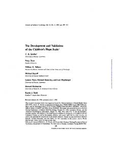
Simplicity. Zone surfaces are defined by their area and orientation. Additional geometric information is required only for solar shading calculations. For cubical enclosures with arbitrary surface emissivities, long-wave radiant exchanges are exactly calculated by the Carroll model. The model is surprisingly accurate for a wide variety of shapes, such as hip roof attics and geodesic domes. Carroll (1981) and CEC (2013) apply four models (some using geometric view factors) to a number of space shapes including one with a 10:1 length-to-width ratio. Comparison of results shows that the Carroll model predictions are within a few percent of exact and have accuracy comparable to those from the other formulations. Carroll’s approach to long wave exchange has been adapted to handle distribution of short wave (solar) radiation as documented in CEC (2013). The zone is approximated as a sphere with diffusely reflecting surfaces. Solar gains from specific windows can be targeted to specific surfaces by user input; all untargeted and reflected radiation is distributed according to surface area, reflectance, and transmittance. Because of the lack of full surface geometry, CSE does not calculate sun patch locations within the zone. Figure 1 shows a simplified schematic of the zone model network. Note the central positions of Ta and Tr which act clearinghouses for convective and radiant exchanges respectively. The following sections describe the modeling approaches for the elements shown in Figure 1. Component models Opaque surface conduction is modeled using a onedimensional forward-difference scheme. A zone can have any number of surfaces. User input specifies construction layer thicknesses and properties. The layers are algorithmically subdivided to yield one or more series-coupled numerically stable “T” networks. This approach inherently captures the short time constant behavior at the construction faces. Each T has heat capacitance centered between two thermal conductances. Conductances can be adjusted by node temperature – this is done for fiberglass insulation, for example. No lateral (2-D) conduction is explicitly modeled (framed constructions are represented as separate surfaces), although 1-D equivalent factors are used for ground contact surfaces (see below) and attic perimeters. The implementation could be easily extended to handle phase-change, open cavities, or other nonstatic “materials.”

- 235 -

Proceedings of BS2013: 13th Conference of International Building Performance Simulation Association, Chambéry, France, August 26-28

AjIjFPj

Qi,c

Construction AiiIi

Windowj AjIjFMj hxi

AjIj

Qi,r j

solar distribution

Figure 1. CSE Zone Network (simplified) Ground contact surfaces are modeled using an approach built on work by Bazjanac et al. (2000) that gives conductances between a fixed zone temperature and moving average outdoor temperatures over several periods. To accommodate varying zone temperature, CSE models 0.6 m (2 ft) of soil coupled to the moving average temperatures via conductances adjusted to preserve to overall values specified by Bazjanac et al. Fenestration. The ASHWAT complex fenestration model is used to represent windows (Barnaby et al. 2009). ASHWAT is a multilayer model that uses a common representation of glazing and shading materials, allowing essentially any combination to be modeled. Wright et al. (2011) describe the integration of ASHWAT into the MRT zone model and show that the fenestration’s complex thermal circuit can be reduced to an equivalent delta shown for the window in Figure 1. ASHWAT additionally calculates the factors FP and FM which are the fractions of window irradiation that is converted to convective and radiant gains by e.g. interior shades. Transmitted solar (short wave) radiation is distributed to zone surfaces. CSE also includes a “ratings matching” scheme that selects and adjusts a multi-layer fenestration assembly to exactly match a rated U-factor and SHGC (Solar Heat Gain Coefficient). This capability is essential in compliance applications, since regulations are generally stated in terms of ratings as opposed to physical construction. Exterior boundary conditions. CSE uses conventional hourly weather files to specify exterior conditions. Several source formats are supported. Time-step values are calculated from hourly

information using linear interpolation. Local wind speed is calculated based on terrain and local shielding using procedures of Sherman and Grimsrud (1980). For conduction through ground-contact surfaces, CSE derives a deep ground temperature and maintains 7, 14, and 31 day moving averages of drybulb temperatures. Sky temperature is modeled using methods developed by Palmiter based on work of Martin and Berdahl (1984) (see Niles et al. 2007 and CEC 2013). Exterior surface convection coefficients are derived from surface tilt, surface temperature, direction of heat flow, and local air velocity. Both natural (temperature difference) and forced (wind) modes are considered. Wind direction effects are implicitly averaged in the models, since local direction is not reliably known. Several alternative models were explored during development and remain available via input choice. Exterior long-wave radiant exchange relies on linearized radiation coefficients derived from surface emissivity, view factors from the surface to the sky and ground, and current temperatures. Ground surface temperature is assumed be the same as air temperature and sky temperature is assumed to approach air temperature at the horizon (Walton 1983). Convection and radiation coefficients are updated each time step. Air temperature, sky temperature, and current coefficients are combined to derive an effective environmental temperature for each surface, simplifying other calculations. Interior boundary conditions. Interior natural convection coefficients depend on surface tilt, surface temperature, and direction of heat flow.

- 236 -

Proceedings of BS2013: 13th Conference of International Building Performance Simulation Association, Chambéry, France, August 26-28 Convective transfer is enhanced as a function of the rate of zone air change from all sources (infiltration, ventilation, and HVAC). Interior radiant exchange uses linearized radiation coefficients that couple surfaces to the zone radiant node (Tr) using the MRT zone model formulation. Internal gains. CSE includes general scheduling capabilities that allow specifying heat gains at any time during the simulation. Gains can be any mix of convective, radiant, or latent and are added to the zone heat and/or moisture balances. Energy consumption represented by gains can be optionally accumulated to a meter (described below).

Zone heat balance CSE uses heat balances to find zone conditions at each time step using procedures detailed in CEC (2013). The following illustrates the basic structure. With reference to Figure 1 and considering only surface and HVAC (Qhc) heat transfers, Equations 1 and 2 can be formed.

 

 

 Ai hci Ti  Ta  C x Tr  Ta   Qhc  0 (1) i  Ai hri Ti  Tr  C x Ta  Tr   0 (2) i In these equations, the novel term Cx is a conductance between Ta and Tr that occurs because some long-wave radiation is absorbed in zone air (depending on zone humidity and mean free path length). Additional contributions to Cx are due to YΔ transforms used to simplify window and surface models. As explained in Y-Δ Transform (2013), three-resistor circuits can be converted from star (Y) to equivalent triangle (Δ) arrangements. This transform is commonly used to simplify electrical circuit analysis and it is useful in thermal problems as well. Equations 1 and 2 are elaborated by adding more terms, grouping, and rearranged to give Equations 3 and 4. Ta 

Qv  Qhc  N a  C xTr Da  C x

(3)

Tr 

N r  C xTa Dr  C x

(4)

Here N and D include all couplings to Ta and Tr such as the surface summations included in Equations 1 and 2, internal gains, and infiltration. At the beginning of each time step, all coefficients (e.g. hci and hri) are updated and the couplings are accumulated to N and D. In some cases prior-step (lagged) values are used. Equations 3 and 4 can then be combined to eliminate Tr, yielding

Ta 

( Qv  Qhc  N a )( Dr  C x )  C x N r ( Da  Dr )C x  Da Dr

(5)

Equation 5 is used to find the uncontrolled (floating) zone air temperature for known conditions or is rearranged to solve for Qhc when the zone air temperature is controlled and thus known. Alternative rearrangements of Equation 5 are used to implement all zone air temperature control situations. Once Ta has been determined, Tr is found using Equation 4. The simplicity of the zone heat balance equations shows how CSE achieves reasonable run times while using short time steps. No simultaneous equations are solved and the accumulation of heat balance terms depends linearly on the number of zone surfaces.

Additional capabilities Zone humidity. A mass balance is used to calculate the zone humidity using water vapor mass that accompanies air transfers. The hygric inertia model of Vereecken et al. (2009) represents the moisture storage effects of zone surfaces and furnishings. When the predicted air moisture content is above saturation, condensation is assumed and corresponding sensible heat is added to the zone air. Surface-specific condensation is not modeled. Comfort. CSE includes an implementation of the PMV-PPD comfort model (ASHRAE 2010). Local air velocity, occupant metabolic rate, and occupant clothing are specified via user input and combined with air dry-bulb temperature (Ta) air humidity, and mean radiant temperature (Tr) to calculate Predicted Mean Vote (PMV) and Predicted Percent Dissatisfied (PPD) at each time step.

AIRFLOW NETWORK To represent air transfers due to infiltration and natural or powered ventilation, CSE models airflows among zones and the outdoors by finding zone pressures that balance all pressure-driven and fixed flows. All defined airflows, such as HVAC supply and return, duct leakage, and ventilation are included in the balances, implicitly capturing the interactions between, for example, HVAC system operation and infiltration. Handling defined flows (e.g. fans and duct leakage) in the network is a matter of accounting. For pressure-dependent leaks, a variety of models are provided (see CEC 2013). Small openings (e.g. infiltration leakage) are modeled with a power law formulation. Large vertical openings (e.g. windows) are represented by two vertically separated openings using the method suggested by Woloszyn and Rusaouën (1999). Large horizontal openings (e.g. stairwells) are modeled methods derived from EnergyPlus (2012) and Cooper (1989).

- 237 -

Proceedings of BS2013: 13th Conference of International Building Performance Simulation Association, Chambéry, France, August 26-28 The simultaneous zone pressures are found with a Newton-Raphson technique, following Lorrenzetti (2002), EnergyPlus, and Clarke and Hensen (1990). Once pressures are known, all flows and thus heat and moisture transfers can be determined and included in zone heat and moisture balances. An important feature of the air network model is that the solution for the current time step does not depend on results from prior step(s). When appropriate, CSE calculates two alternative air network solutions, one without ventilation and another with ventilation (windows open or fans operating). The zone temperature control algorithm then determines a fractional intermediate ventilation operating mode.

HVAC MODELS Simple correlation-based residential equipment models have been implemented in CSE for airconditioners, air-source heat pumps, and furnaces. These require only standard U.S. ratings as input. For example, the air-conditioning model needs only the total cooling capacity at 95 °F outdoor dry-bulb temperature and SEER (Seasonal Energy Efficiency Ratio). The equipment models are sensitive to airflow rate, entering air state (temperature and humidity), and outdoor dry-bulb temperature. The models are intended to adequately represent performance for code compliance purposes without requiring input data that are typically difficult to obtain. The CSE duct model builds on procedures given by Fransisco and Palmiter (1999 / 2003). Supply and return ducts can be independently located in any conditioned or unconditioned zone or outdoors. Conduction losses are determined by treating each duct run as a heat exhanger with known surrounding conditions and entering air temperature. The heat exchange with the surroundings and the leaving air temperature are calculated with a classical NTU model. Leakage mixes surrounding air into the duct stream (for return ducts) or adds duct air to the surrounding zone (for supply ducts). Duct leakage is included in the airflow network as fixed flows (that is, surrounding zone pressure does not alter leakage rates). Because both conduction and leakage are correctly included in the surrounding zone heat and airflow balances, the overall impact of distribution ducts can be realistically evaluated. An autosizing capability is available that allows CSE to find required equipment capacities based on design-day weather.

IMPLEMENTATION CSE is implemented in standard C++ and runs as a Microsoft Windows console application. Porting to other platforms should be straightforward but remains to be attempted. Execution speed is reasonable, given the short time steps and the computation involved in the airflow network model. Typical run times on a 2012-vintage PC are on the

order of 30 seconds for a two zone building (conditioned zone + attic). The program operates as a batch-mode application. Input is taken from a text file that uses a simple but powerful keyword-style language. Most of the features of the C pre-processor are supported, such as conditional text, macros, and inclusion of external files. In addition, a runtime expression feature allows many inputs to be varied during the simulation. Expressions can refer to internal simulation values using “probes” indicated by an @ prefix. Thus, it is possible to specify sfExtT = @zone[“attic”].tz + 20

to indicate the temperature adjacent to a surface should be the attic air temperature + 20. Expression evaluation occurs automatically at intervals required by the variability of the terms in the expression. The expression capability has proven extremely valuable for model prototyping and software testing. Meters are another powerful feature, allowing flexible accumulation and reporting of energy consumption categorized by end-use. Several standard output reports are implemented. User-defined reports can be constructed using expressions and probes to group results as required. Output can be directed to formatted files, commaseparated text files (convenient for import into spreadsheets or other downstream tools), or binary files.

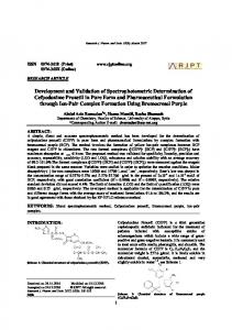
CENTRAL VALLEY RESEARCH HOMES The Central Valley Research Homes Project (CVRH) is operating four unoccupied, heavily instrumented research homes in Stockton, California. Stockton, located in California’s central valley, has hot dry summers and moderately cold winters that represent the climate challenge of inland California. The CVRH houses were built in 1948, 1953, 1996 and 2005 (shown in Figure 2). They have features found in typical older California homes including single glazing, uninsulated construction, and leaky ducts in unconditioned attics. The first year of operation (2012 – 2013) is providing baseline data on how older homes actually work. In the spring of 2013, each house will be upgraded with an efficiency package designed to save 75% of the heating and cooling energy. An additional 2 years of operation will then measure the actual savings. In addition to providing a demonstration of the potential for deep energy retrofits, the project is designed to provide detailed data to support development and validation of improved computer models for energy code compliance and home energy ratings.

- 238 -

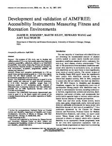
Proceedings of BS2013: 13th Conference of International Building Performance Simulation Association, Chambéry, France, August 26-28 Figure 4 shows a daily cooling consumption for the 1996 home with some days cooled with the reference system and others with the existing (old) system. The old system is strikingly less efficient and highlights the importance of keeping a constant reference system during retrofit experiments of this type. Comparisons of CSE simulations and measured results are underway. Figure 5 shows a preliminary comparison of measured daily reference system cooling energy for the 2005 CVRH home over a range of conditions. Measured and simulated results show reasonably good correspondence; detailed investigation of differences remains to be completed. Detailed daily and hourly comparisons will be performed for both hot and cold weather conditions.

Figure 2 CVRH laboratory home built in 2005

- 239 -

Figure 3. Reference air conditioning system

37 33 29

kW hours/day

Instrumentation measures space temperatures, weather data, and energy use at 1 minute intervals. Energy use is measured with true-power watt meters and utility grade gas meters, temperatures are measured with asperated and shielded thermocouples, and solar radiation is observed with a class 2 pyranometer. Slab heat flow is also measured at one house. A formal uncertainty analysis has not been performed, but overall, the instrumentation quality is very good and observations are routinely checked for plausibility and internal consistency. The CVRH project is designed to solve the problems in using field data for validating computer simulations. Occupied homes present the problem of variable occupant activity that can confound comparisons with modeled behavior. The unoccupied CVRH houses eliminate this issue by using computer controlled simulated occupancy that exactly matches the model assumptions. Separating the effects of simultaneous changes in envelope and HVAC systems is made possible by the use of special reference heating and cooling systems that are installed as part of the experimental measurement apparatus. The reference systems are located entirely in the conditioned space (for example, see Figure 3) so they have no duct losses and are designed so that the heating and cooling output can be easily measured. The reference systems will be maintained as constant throughout the project and operated on alternate sets of days with the existing system (as found and later upgraded). Comparison of reference system loads before and after the envelope upgrades can be used to establish the separate impact of envelope upgrades alone. The existing and upgraded HVAC energy consumption can be compared to the energy consumption of the reference system to establish relative efficiency.

25 21

OLD 17

REF.

13 9 5 1 75

80

85

90

95

100

105

Max Outdoor Temperature, F

Figure 4. 2012 old and reference daily cooling energy for the 1996 CVRH home

Proceedings of BS2013: 13th Conference of International Building Performance Simulation Association, Chambéry, France, August 26-28 16

140

Simulation

Measured

Total

14 120

12 100

kWh/day

10 80

8

60

6

4

40

2 20

0 11

12

15

16

19

20

23

24 27 28 Day Starting Aug 10

31

1

4

8

9

12 0

Figure 5. CSE simulated and measured daily cooling energy for a CVRH Home

CONCLUSIONS AND FUTURE WORK A number of conclusions can be drawn from the CSE development project.



The use of short time steps and forward difference numerical techniques is an accurate and practical simulation strategy. Short time constant phenomena are accurately captured. Iteration within time steps is rarely required.



Modeling residential buildings requires representing subtle effects in a few zones as opposed to handling many zones with controlled conditions (the typical non-residential case). Natural ventilation, ground heat transfer, and interzone air leakage are generally important in residences. CSE has strong capabilities in all these areas.



Even engines should be friendly. Features such as readable input formats, runtime expressions, macros, and flexible output are not strictly required for applications intended to be embedding within user interface frameworks. However, such features substantially increase productivity of development, prototyping, and testing.



C++ is a highly suitable language for simulation engine development. The object-oriented, data manipulation, and memory management capabilities of C++ are well matched to building modeling problems. Numeric performance is comparable to FORTRAN. As of mid-2013, work is underway to prepare CSE and associated software for use in compliance with the California residential energy standards for new buildings that go into effect in January 2014. Testing against ASHRAE Standard 140 (ASHRAE 2011) is planned. California energy agencies are collorating to establish a BEopt / CSE interface (Christensen 2006).

Over the next two years work will continue with the CVRH data to improve calculation procedures and algorithms for both new and existing homes. The CVRH data set will include detailed measurements for both the unimproved (as found) and extensively upgraded versions of the 4 homes. We believe this will provide an unprecedented software validation resource.

AVAILABILITY The CSE executable beta and support documents are available at www.energydataweb.com/consortium/ PACdocs.aspx. Source code for all compliance software, including CSE, will be available on an open source basis via procedures to be promulgated by the California Energy Commission. Contact the authors for information about obtaining source code, CVRH data sets, and documentation.

NOMENCLATURE = area, m2 (ft2) = zone effective heat capacity (optionally represent e.g. furniture), Wh/°C (Btu/°F) Ci,k = heat capacity of kth construction layer, Wh/°C (Btu/°F) Cx = Ta-to-Tr coupling, W/°C (Btu/h-°F) ccw = fenestration effective conductance to zone air temperature, W/°C (Btu/h-°F) crw = fenestration effective conductance to zone radiant temperature, W/°C (Btu/h-°F) D = zone heat balance denominator term, W/°C (Btu/h-°F) FM, FP = fenestration solar gain conversion factors (see text) hc = convection heat transfer coefficient, W/m2-°C (Btu/h-ft2-°F) hr = linearized radiation heat transfer coefficient, W/m2-°C (Btu/h-ft2-°F) hx = exterior surface combined convectiveradiant heat transfer coefficient, W/m2-°C (Btu/h-ft2-°F)

A Ca

- 240 -

Proceedings of BS2013: 13th Conference of International Building Performance Simulation Association, Chambéry, France, August 26-28 i, j I N Qhc Qi Qs Qv Ta Teo Ti,k Tr

 

= surface indicies = Incident solar radiation, W (Btu/h) = zone heat balance numerator term, W (Btu/h) = HVAC heat gain, W (Btu/h) = internal (casual) gain, W (Btu/h) = surface solar gain, W/m2 (Btu/h-ft2) = ventilation heat gain, W (Btu/h) = zone air temperature, °C (°F) = effective environmental temperature, °C (°F) = temperature of kth construction layer, °C (°F) = zone radiant temperature, °C (°F) = absortance = transmittance

Christensen, C., R. Anderson, S. Horowitz, A. Courtney, and J. Spencer. 2006. BEopt™ Software for Building Energy Optimization: Features and Capabilities. NREL/TP-550-39929. http://www.nrel.gov/docs/fy06osti/39929.pdf. See also beopt.nrel.gov.

ACKNOWLEDGEMENT We gratefully acknowledge financial support from the California Energy Commission (CEC), Pacific Gas & Electric Company, Southern California Edison, and Sempra Utilities.

REFERENCES ASHRAE. 2010. Thermal Environmental Conditions for Human Occupancy, Appendix D (Computer Program for Calculation of PMV-PPD). ANSI/ASHRAE Standard 55-2010. ASHRAE, Atlanta, GA. ASHRAE. 2011. Standard 140-2011 – Standard Method of Test for the Evaluation of Building Energy Analysis Computer Programs. ASHRAE, Atlanta, GA. Balcomb, J. D. 1997. Energy-10: A Design Tool Computer Program. Building Simulation 1997 (Prague), IBPSA (accessible at www.ibpsa.org) Barnaby, C. S., Wright, J. L., Collins, M. R., 2009. Improving Load Calculations for Fenestration with Shading Devices, ASHRAE Transactions, Vol. 115, Pt. 2, pp. 31-44. Bazjanac V., J. Huang, and F. C. Winkelmann. 2000. DOE-2 Modeling of Two-dimensional Heat Flow in Underground Surfaces. California Energy Commission. Carroll, J. A., 1980. An ‘MRT Method’ of Computing Radiant Energy Exchange in Rooms, Proc. Second Systems Simulation and Economic Analysis Conference, San Diego, CA. Carroll, J. A., 1981. A Comparison of Radiant Interchange Algorithms, Proc. ASME Solar Energy Division 3rd Annual Conf. on Systems Simulation, Economic Analysis/Solar Heating and Cooling Operational Results, Reno, NV. CEC. 2013. 2013 Residential Alternative Calculation Method: Algorithms. California Energy Comission. http://www.energy.ca.gov/title24/ 2013standards/implementation/documents/

Clarke, J.A. and J.L.M. Hensen. 1990. An Approach to the Simulation of Coupled Heat and Mass Flows in Buildings. 11th AIVC Conference, Belgirate, Italy. Cooper, L.Y. 1989. Calculation of the Flow Through a Horizontal Ceiling/Floor Vent. NISTIR 894052. EnergyPlus. 2012. EnergyPlus Engineering Reference. http://apps1.eere.energy.gov/ buildings/energyplus/pdfs/engineeringreference. pdf Francisco, P.W. and L. Palmiter. 1999 (revised 2003). Improvements to ASHRAE Standard 152P. U.S. DOE Subcontract 324269-AU1. Lorenzetti, D. M. 2002. Computational Aspects of Multizone Airflow Systems. Building and Environment 37, p. 1083 – 1090. Martin, M. and P. Berdahl. 1984. Characteristics of Infrared Sky Radiation in the United States. Solar Energy Vol. 33, No. 3/4, pp 321-336. Niles, P., L. Palmiter, B. Wilcox, and K. Nittler. 2007. Unconditioned Zone Model. PIER Research for the 2008 Residential Building Standards. CEC-400-2007-021. See http://www.energy.ca.gov/2007publications/CE C-400-2007-021/CEC-400-2007-021.PDF Sherman, M.H. and D. T. Grimsrud. 1980. Measurement of Infiltration Using Fan Pressurization and Weather Data. LBL-10852. Vereecken, E., S. Roels, and H. Janssen. 2009. In Situ Determination of the Moisture Buffering Potential of Room Enclosures. Building Simulation 2009 (Glasgow), IBPSA (accessible at www.ibpsa.org). Walton, G.N. 1983. Thermal Analysis Research Program Reference Manual. NBSSIR 83-2655. National Bureau of Standards. Woloszyn, M. and G. Rusaouën. 1999. Airflow Through Large Vertical Openings in Multizone Modelling. Building Simulation 1999 (Kyoto), IBPSA (accessible at www.ibpsa.org). Wright, J. L., C. S. Barnaby, P. Niles, and C. Rogalsky. Efficient Simulation of Complex Fenestration Systems in Heat Balance Room Models. Building Simulation 2013 (Sydney), IBPSA (accessible at www.ibpsa.org). Y-Δ Transform. 2013. http://en.wikipedia.org/wiki/ Y-Δ_transform.

- 241 -