Project Report No. 388 (Appendices A - K Pgs 49 - 127) February 2006
Development and validation of ‘Weed Management Support System’ (Weed Manager) by LV Tatnell1, JH Clarke1, D Ginsburg1, PJW Lutman2, A Mayes2, L Benjamin2, DJ Parsons3, AE Milne3, DJ Wilkinson3, DHK Davies4 1
2
ADAS Boxworth, Battlegate Road, Boxworth, Cambridge CB3 8NN Rothamsted Research, West Common, Harpenden, Hertfordshire AL5 2JQ 3 Silsoe Research Institute, Wrest Park, Silsoe, Beds, MK45 5HS 4 Scottish Agricultural College, Kings Buildings, West Mains Road Edinburgh, Midlothian EH9 3JG
Weed Manager was a collaborative Sustainable Arable LINK (LK0916) project between ADAS, Rothamsted Research, Silsoe Research Institute and SAC that ran for 5 years, starting in October 2000 and ending in September 2005. Defra (£812,052, through SA LINK) and HGCA (£373,022, project 2286) sponsored the project, with industrial support from Bayer CropScience (£158,868), BASF (£150,255), Dow AgroSciences (£155,320), DuPont (£150,255), and Syngenta Crop Protection UK (£304,351). The total cost of the project was £2,104,123.
The Home-Grown Cereals Authority (HGCA) has provided funding for this project but has not conducted the research or written this report. While the authors have worked on the best information available to them, neither HGCA nor the authors shall in any event be liable for any loss, damage or injury howsoever suffered directly or indirectly in relation to the report or the research on which it is based. Reference herein to trade names and proprietary products without stating that they are protected does not imply that they may be regarded as unprotected and thus free for general use. No endorsement of named products is intended nor is it any criticism implied of other alternative, but unnamed, products.
6.0 APPENDICES A: B: C: D:
Herbicide Screening experiments Field validation trials Weed Manager Encyclopaedia (Draft paper version 3 ) A model to simulate the growth, development and competitive effect of weeds in a winter wheat crop in the UK (Draft paper version 3) E: Modelling weed management over a rotation in the UK using stochastic dynamic programming (Draft paper ) F: A model based algorithm for selecting weed control strategies that maximise profit margin in winter wheat (Draft paper) G: System architecture – A summary H: The resistance module summary I: Example page from a herbicide spreadsheet for product Ally J: Technology Transfer for Weed Manager K: A spray nozzle selection support system for herbicide applications L: User reports by Glasgow Caledonian University WMSS User Group Activities - November 2002 to March 2003 WMSS Training Session Results - December 2003 WMSS User Interview results, Field based trials - October 2004 The WMSS Heuristic Evaluation – June 2004
50 52 59 67 83 98 107 115 119 120 122
1 12 18 57
*Appendix L is available electronically on the HGCA website, and does not form part of the printed report.
49
APPENDIX A Herbicide Screening experiments Materials and Methods Trial design, planting and maintenance The herbicide screen was blocked by herbicide, and there were three replicate blocks. Ten seeds of each weed species (Table 1) were sown into individual 3’ plastic plant pots containing John Innes No. 2 (low OM sterilised soil) and pots were thinned to 3 plants per pot when seedling emerged. Pots were maintained in the glasshouse under the conditions of 18oC day temperature with 12 hours daylight and 10oC at night. The benches were covered with capillary matting to allow watering from below, and initially the pots were covered with clear plastic to prevent the seedlings drying out.
Table 1 The list of weed species tested in the glasshouse herbicide screening experiments. BAYER code Latin name SCAPV Scandix pecten-veneris ANTAR Anthemis arvensis ANTCO Anthemis cotula BRSNI Brassica nigra CENCY Centaurea cyanus CENNI Centaura nigra CERVU Cerastium vulgatum CHYLE Leucanthemum vulgare DAUCA Dauca carota ECHVU Echium vulgare GAESE Galeopsis speciosa GASPA Galinsoga parviflora LYCAR Anchusa arvensis MATCH Matricaria recutita MELAL Silene latifolia PAPDU Papaver dubium PAPHY Papaver hybridum RANAR Rananculus arvensis RESLU Reseda lutea SSYOF Sisymbrium officinale STEME* Stellaria media POANN* Poa annua * standard weed species used at both sites
Common name Shepherd's-needle Corn chamomile Stinking chamomile Black mustard Cornflower Knapweed Common mouse-ear Oxeye daisy Wild carrot Viper’s-bugloss Large flowered hempnettle Gallant soldier Bugloss Scented mayweed White campion Long-headed poppy Rough poppy Corn buttercup Wild mignonette Hedge mustard Common chickweed Annual meadow grass
Herbicide applications For the post-emergence herbicides the plants were sprayed when they had reached approximately the 3-leaf stage, which required grouping the species into 3 different spray batches based on their growth stage. The 3 replicates were sprayed in a covered polytunnel using a knapsack sprayer, fitted with a 1m wide boom with flat fan nozzles, at a spray pressure of 2-3 bar, applied at a rate of 200 l water /ha. The products were applied at two rates of the chemical, normal field rate and half field rate (Table 2).
50
Table 2 Herbicide treatments and application rates for glasshouse screening experiments. Application rates Herbicide product Active ingredient Full field rate Half rate Eagle Amidosulfuron 40.0 g/ha 20.0 g/ha Harmony -M Thifensulfuron 60.0 g/ha 30.0 g/ha Lexus Flufensulfuron 15.0 g/ha 7.5 g/ha BASF MCPA MCPA 3.0 l/ha 1.5 l/ha Duplosan Mecoprop-P 2.0 l/ha 1.0 l/ha Quantum Tribenuron 20.0 g/ha 10.0 g/ha Boxer Flurasulam 0.15 l/ha 0.075 l/ha Picopro Picolinofen + PDM 2.0 l/ha 1.0 l/ha Oxytril Bromoxynil/Ioxynil 1.5 l/ha 0.75 l/ha Lotus Cinodon-ethyl 0.25 l/ha 0.125 l/ha Starane 2 Fluroxypyr 1.0 l/ha 0.5 l/ha Dow Shield Clopyralid 1.0 l/ha 0.5 l/ha Arelon Isoproturon 4.2 l/ha 2.1 l/ha Panther DFF + IPU 2.0 l/ha 1.0 l/ha Crystal Flufenacet + PDM 2.0 l/ha 1.0 l/ha Fortrol Cyanazine 2.5 l/ha 1.25 l/ha Treflan Trifluralin 2.3 l/ha 1.15 l/ha Avadex Excel 15G Tri-allate 15.0 kg/ha 7.5 kg/ha Ally* Metsulfuron 30.0 g/ha 15.0 g/ha Stomp* Pendimethalin 1.5 kg/ha 0.75 kg/ha * standard herbicides used at both sites Assessments Post-spraying the pots were returned to the glasshouse and assessed 1-2, 5-7, 14-16 and 21-24 days after treatment for any herbicidal effect. Assessments were on a visual % damage basis, using the 09 scale Results The results from the herbicide screening experiments are displayed within the system on the relevant herbicide or weed page, called additional information. These data are for reference only and are not included in any decision making processes.
51
APPENDIX B Field validation trials Materials and Methods In the autumn of 2002 field trials were established (Table 1) in a crop of winter wheat at two different ADAS sites, Boxworth (Cambridgeshire) and Rosemaund (Herefordshire) and at SAC in Edinburgh. In 2003 two trials were established at ADAS Boxworth only (Table 1). Fields were selected with a low natural weed population and the desired weed species were hand sown. Table 1. The location and weed species chosen for each field trial site. Species/trial year Sites ADAS Boxworth SAC ADAS Rosemaund Black-grass 2002/03 aa Black-grass 2003/04 a* Chickweed 2002/03 a a Cleavers 2002/03 a aa Cleavers 2003/04 a aarepresents two drilling dates for that particular experiment. *individual plots were selected from a large black-grass trial, with a natural population of blackgrass, therefore no specific trial was sown for this project in 2003/04. Where two drilling dates were required the target drilling dates were late September and late November. No herbicide treatments were applied other than the trial treatments, but all other farm inputs were to standard commercial practice for that particular farm. Trial design For the trials with multiple drilling date a split plot design was used, with 3 main blocks for the 3 replicates, sub-divided into 2 blocks in each main blocks for the drilling dates and sub-plots for the combinations of herbicide programme and weed density. Trials with a single drilling date were a randomised block design. The minimum plot size was 3m x 12m. Weed density The densities for each species (Table 2) were selected to cover a range where the models predict that the rate of change of crop yield with weed density is at its highest. Weed seed was hand sown into each plot on the day of drilling ahead of a commercial crop of winter wheat being sown. Weed seeds were purchased from Herbiseed, UK and were known to be from non-resistant populations. Table 2 The weed species target densities for the field validation trials Density (plants per m2) Weed species Low Medium Black-grass 6 36 Chickweed 6 36 Cleavers 4 16
High 216 216 64
Herbicide treatments Application timings of the herbicide treatments were determined by the growth stage of the weed species. The early herbicide treatment was applied at 2-leaf growth stage of the crop, and the late treatment at the 8-leaf stage and after canopy closure. The choice of herbicide products and doses were weed dependent and are presented in Table 3. Herbicides were applied using a knapsack sprayer and 3m boom, with Lurmark 02 F110 nozzles, at a rate of 200L water/ha and a pressure of 3.0 bar.
52
Table 3 The herbicide treatments, application timings and dose rates. Weed species Treatment Timing Application Timing Herbicide Chickweed
Black-grass
Early Late
Post-em (autumn) GS30 (after 1st Feb)
Treflan Ally (+ Starane)*
Full control
Autumn (Ally-Spring, after 1st Feb) Autumn (up to 2-3 tillers) Feb/March Autumn post-em Autumn 2-3 lvs.
Panther (fb. Ally if needed) Lexus 50DF
Early Late Full control
Cleavers
Early Late Full control
Autumn Feb/March Autumn Crop GS 31-32 Autumn Spring
Topik Crystal Hawk + Lexus 50DF IPU Eagle IPU Starane (+Ally if needed) Panther Starane
Rate 2.0 l/ha 7.5g/ha l/ha)* 2.0 l/ha (30g/ha) 20 g/ha
0.16 l/ha 4.0 l/ha 2.5 l/ha + 20g/ha 3.0 l/ha 20 g/ha 3.0 l/ha 0.5 l/ha 2.0 l/ha 1.0 l/ha
Assessments Within each plot one 0.5 m2 permanent quadrat was marked out for seedling emergence (of crop and weeds) counts. Up to 4 other 0.5 m2 quadrats per plot were destructively sampled as detailed below:i) Seedling Emergence Counts On one of the weed density plots in each replicate, the number of weed and wheat seedlings was counted every 3 or 4 days, depending on the change in numbers observed, until emergence was complete. When emergence is complete, the numbers of seedlings in a sample quadrat in each plot should be recorded to determine the density of weeds. ii) Biomass assessments and GAI assessments On the no herbicide application treatments only, a visual assessment of the ground cover was recorded in one 0.5 m2 permanent quadrat and all plants were hand harvested and separated into the different species. Individual weeds and crops were counted and a growth stage measurement of weed and crop was assessed and recorded by selecting 6 representative plants from each species. For each species (all weeds including natural populations and crop), the leaves and stems were separated and the green area measured. This process was repeated at each of the following timings on the appropriate plots:• Three weeks after Early Herbicide Application (when symptoms of treatment were visible) • At Canopy Closure (defined as when the GAI of all weeds plus crop reaches 0.75). • Three weeks after Late Herbicide Application (when symptoms of herbicide treatments were visible) • June (before combining the plot) – all plots. iii) Final Crop Yield Harvest from combine yield area The fertile tillers were counted in each plot using each side of a 0.5m rod placed between the crop rows at 5 points per plot. Plots were harvested using a Sampo plot combine and plots length measurements were recorded. Sample of grain were collected and processed for grain moisture content and a thousand grain weight. Plot yields were calculated. Data analysis The data collected from measurements were entered into EXCEL spreadsheets and sent to Rothamsted for further collation and analysis. Given the GAI observed at complete seedling 53
(0.5
establishment and daily meteorological records, a model of green area expansion was run in Matlab to predict the GAI at canopy closure in the no herbicide control treatments. The model used parameter values from the literature. These simulations were used to predict the weed GAI before herbicide application. The difference between this value and that observed after applications was compared with the expected efficacy of the herbicide. The ratio of weed species GAI to winter wheat GAI at canopy closure was used as inputs to the equations used to relate these ratios to winter wheat yield loss. Statistical Analysis of Observed Data The times of weed and crop seedling establishment were estimated by fitting logistic curve to the seedling numbers observed in the permanent quadrats. The yield of the winter wheat at harvest, the biomass of each weed species prior to harvest and the GAI of each sown species at emergence, canopy closure was subjected to an ANOVA in Gentstat. Regressions between visual assessments of cover and GAI were conducted. The differences between observed and predicted winter wheat yield loss and between observed and predicted GAI at emergence and canopy closure, were also subjected to an ANOVA. Additionally, the simulation models were fitted separately to each replicate and the fitted values subjected to an ANOVA. Results The results from the field trials were evaluated by the experts and tested against the model outputs. Comparison of the predicted and observed crop growth stages from the first season (2002-03) showed good agreement. The model was compared with data from the black-grass trial at ADAS Boxworth on crop and weed green area index (GAI) and the effect of weeds and herbicide treatments on crop yield. Autumn 2002 was very dry, leading to exceptionally low germination of the weeds. The model predicted slightly higher germination rates and consequently higher weed GAI than were observed. The weed densities were so low that the differences between treatments (weed sowing density and herbicide programme) were not significant. The predicted yields were lower than the mean observed yields, but these differences also were not significant. Inspection of the data showed similarly low GAIs for the other weed species, so the testing was not repeated, as it was unlikely to show additional information. The second season (2003-04) included fewer weed species, but the weather conditions gave rise to high weed populations resulting in significant yield losses. The model was assessed on the basis of yield loss in sprayed and unsprayed plots (using several spray programmes), thus testing the combined effects of all the steps in the model. Examples of the results are summarised below from the 2003/04 cleaver and black-grass trials. Cleaver trial 2003/04 ADAS Boxworth Crop Sown Previous harvest Cultivation Density sown Potential yield
Wheat 14 Nov 2003 31 Aug 2003 (assumed) Direct drill (assumed) 200-300 based on emergence data 10.6 t/ha (see yield table below)
Weed Sown Density sown
Cleavers 14 Nov 2004 low = 4 medium = 16
high = 64
54
Plant Emergence (mean over treatments) Date Crop Weed density density low 15/12/03 213 2 22/12/03 269 4 5/01/04 278 15 12/01/04 294 21 19/01/04 299 26 2/02/04 301 29 13/02/04 289 30
Weed density medium 9 16 50 73 81 87 83
Weed density high 35 71 182 238 265 273 263
Spray programmes (table from protocol; dates from diary) Treatment Timing
Application Timing
Herbicide
Rate
Early
08/12/03
IPU (6159)
3.0 l/ha
Late
04/03/05 08/12/03
Eagle (6131) IPU (6159)
20g /ha 3.0 l/ha 0.5 l/ha
Untreated
02/05/04 Starane (7370) Pre-emergence spray only
Full control
08/12/03
Panther (6128)
2.0 l/ha
13/04/04
Starane (7370)
1.0 l/ha
All include 05/12/03 – Pre-emergence spray to kill black-grass – Topik and Avadex. System data: Topik ID = 8 (with adjuvant), Dose = 1.0; Avadex ID = 7419, Dose = no data – omit Eagle doses are 0.03 and 0.04 – use 0.03 on the assumption units are kg. Starane 2 doses are 0.75, 1.0, 2.0 – use 0.75 in place of 0.5 Cleavers trial results – yield t/ha Weed density sown Sprays None Untreated Early Late Full 10.17-11.15 (10.61)
Low 9.75-10.73 (10.17) 10.42-10.84 (10.63) 9.86-10.84 (10.29)
Medium 8.67-9.70 (9.10) 9.19-11.25 (10.29) 9.86-10.58 (10.32)
High 7.17-9.60 (8.51) 10.01-10.63 (10.37) 9.96-10.84 (10.37)
Model runs Used Bedford weather (closest available DESSAC site), with gaps filled by Wittering weather site. Cleavers model results (parameter set 1.02) – yield t/ha Weed density sown Sprays None Low Medium Untreated 10.54-10.60 8.23-9.00 5.01-6.09 Early 10.60 10.34-10.43 9.66-9.99 Late 10.54-10.60 8.27-9.00 5.06-6.15 Full 10.60 10.54-10.56 10.36-10.44
55
High 2.04-2.79 7.80-8.58 2.08-2.83 9.77-10.04
Comments • The yield losses in the model from uncontrolled cleavers were far higher than observed. • The control obtained by the late spray programme was far less than observed. • Therefore, in order for it to have an effect, the second treatment had to be brought forward to March. With this timing, the yield is similar to that from the Early programme. This was thought to be a feature of the model. The model was tested using the alternative parameter sets that were considered on 8 March: 1.04 – emergence refitted by Jonathan Storkey, rejected because of large changes in many weeds 1.05 – other parameters fitted by Laurence Benjamin using PCA – small changes to most weeds 1.06 – combination of 1.04 and 1.05 Cleavers model results (parameter set 1.04) – yield t/ha Sprays Weed density sown None Low Medium High Untreated 10.60 10.36-10.45 9.74-10.03 7.84-8.61 Early 10.60 10.58-10.59 10.52-10.55 10.28-10.39 Late 10.60 10.37-10.45 9.76-10.04 7.88-8.64 Full 10.60 10.60 10.58-10.59 10.52-10.55 Cleavers model results (parameter set 1.06) – yield t/ha Sprays Weed density sown None Low Medium High Untreated 10.60 10.26-10.38 9.36-8.76 6.91-7.84 Early 10.60 10.44-10.50 10.00-10.20 8.54-9.16 Late 10.60 10.27-10.39 9.38-9.78 6.96-7.88 Full 10.60 10.60 10.56-10.57 10.44-10.50 Parameter set 1.05 gave even lower yields than 1.02. Comments • The evidence is insufficient to recommend a change of parameter sets, especially as the results for black-grass (see below) are different. Further investigation of GAI, etc was required before a decision was made whether the fault is with weed development, crop development or competition. Black-grass trial (ADAS Boxworth 2003/04) Crop Sown Previous harvest Cultivation Density sown Potential yield
Wheat 16 Oct 2003 31 Aug 2003 (assumed) Direct drill (assumed) 150-250 based on emergence data 9.2 t/ha (see yield table below)
Weed Black-grass Sown Natural population Density 100-250 based on early emergence Emergence Date 4/02/04 27/04/04 6/07/07
Crop density untreated 162-286 (239) 168-244 (202) 128-182 (155)
Crop density sprayed 144-358 (260) 216-316 (253) 180-218 (200)
56
Weed density untreated 98-240 (144) 208-506 (388) 124-212 (168)
Spray programmes (table from protocol; dates from diary) Treatment Timing
Application Timing
Herbicide
Rate
Early (T4 from BG slots trial) Late (T20 from BG slots trial) Untreated (T44 from BG slots)
02/12/03
Lexus 50DF + Stomp [+Fortune] (6141) + (7214)
20 g/ha + 3.3 l/ha [+ 1.0 l/ha]
23/01/04
Atlantis [+ BioPower] (7185)
0.4Kg/ha [+ 1.0 l/ha]
Full control
21/10/03
Use untreated plots from black-grass slots trial 2004
18/12/03
Crystal (6130) Hawk + Lexus [+Fortune] (6134) + (6141)
4.0 l/ha 2.5 l/ha + 20g/ha [+ 1.0 l/ha]
From system Lexus 50DF dose 0.02 Stomp 400 EC dose 3.3 Atlantis WG no data Crystal dose 4.0 Hawk no data Hawk = clodinafop-propargyl + trifluralin 12.383 g/l clodinafop-propargyl = Topik (250 g/l, ID = 8 (with adj), dose = 1) trifluralin = Alpha Trifluralin (480 g/l, ID = 6148, dose = 2.3) Black-grass trial results Treatment Timing Untreated Early spray Late spray Full control
Yield t/ha 2.13-6.47 (4.91) 5.38-9.03 (7.12) 8.2-9.11(8.73) 8.59-9.77 (9.21)
Model runs Used Bedford weather (closest available DESSAC site), with gaps filled by Wittering. Black-grass model results (parameter set 1.02) – yield t/ha Treatment Timing Sensitive Resistant Untreated 6.44-8.48 6.44-8.48 Early 8.61-9.14 8.25-9.07 Late * * Full 9.00-9.18* 8.66-9.14* *Unable to simulate the late programme due to the absence of data for Atlantis. Full programme used mixture in place of Hawk due to absence of data. Comments • The yield losses from untreated or partly controlled black-grass are too low. • Parameters sets 1.04 and 1.06 increased the mean untreated yield to 9.0. Set 1.05 reduced it to 6.67, which is still high.
57
If the density is increased to 250-500 (the range for late emergence) the results are Black-grass model results (parameter set 1.02, high density) – yield t/ha Treatment Timing Resistant Untreated 4.95-7.36 Early 7.52-8.75 Late * Full 8.21-8.98 Comments • These are closer to the trials, but still on the high side for untreated, and required very high densities. The potential yield probably should be increased, given that the maximum with the full treatment is lower than observed, which would then raise all the yields. • We need to look at the leaf areas, etc., but these results tend to suggest that black-grass should be made more competitive in the model.
58
APPENDIX C
Draft paper version 3 on 05/12/05
Weed Manager Encyclopaedia D. Ginsburg ADAS Boxworth, Boxworth, Cambridge, CB3 8NN Abstract Weed Manager is a decision support system running within the ArableDS data sharing environment to assist farmers and their advisors with weed related issues within a wheat cropping season and over a six year rotation. The weed manager uses databases to deliver data to the Weed Manager mathematical models. These data are also available to users through the encyclopaedia thus increasing their confidence in the system. Most of the other encyclopaedic information is stored in the database and is viewed with a combination of static and dynamic pages, some of which are wholly or partially database driven. User input in the design process has resulted in an intuitive and easily navigated system. Introduction Weed manager was developed to aid people working in the agricultural industry with decisions about weed management in a single crop of winter wheat (within-season module) or in an arable rotation (rotational module). The program was developed to run within the ArableDS data-sharing environment to share common information about pesticides, weather and farm data. (Parsons et al,2004,). The previous ArableDS modules have been released with background information in the form of an encyclopaedia. Parker and Clarke (2001) have argued that users were more confident in the use of decision support systems when fully aware of the information used to predict outcomes. The primary aim of the encyclopaedia was to make information used in the rotational and within season modules available to the user by sharing information across the system. The data used by Weed Manager and the common data provided to the ArableDS decision support modules change frequently so are held in databases. Background information about weeds and herbicides also needed to be collected and displayed There are various internet sites that show information on weeds. For example ‘The Arable Seed Identification System’ (http://www.scri.sari.ac.uk/asis/) and ‘The Ecological Flora of the British Isles’ (http://www.york.ac.uk/res/ecoflora/cfm/ecofl/index.cfm, and some PC based programmes such as Hypermedia for Plant Protection (INRA) are available, but no electronic encyclopaedia dealing with all weed related issues exists. The weed manager encyclopaedia was developed to co-locate and display all this information satisfying three criteria: 1. To increase user confidence in Weed Manager. 2. To provide a simple interface that would be user friendly and intuitive and incorporated user requests. 3. Be easy to update. Methodology Design criteria and approach Previous ArableDS module encyclopaedias (in Wheat Disease Manager and Oilseed Rape Pest Manager) have information on both pesticide products and their targets, so the Weed Manager encyclopaedia needed to display information both on herbicide products and on weeds (defined as arable non-crop plants). In order to increase confidence in the system, it was necessary to make information used in the rotational and within-season modules available to the user and to respond to their-requests for particular data and types of data display.
59
This led to a two direction approach; effective system design exploited the data needs of both the system and encyclopaedia, while user-consultation helped define and refine both information displayed and the user interface. User input An iterative user consultation process was carried out (Park, Parker and Ginsberg, 2004). Users requested the following information: Herbicides Basic information on products Some information on tank mixes and adjuvants Off-label information Efficacy information from other sources Environmental information Weeds A single, up to date source of weed biology. Basic information on the full range of weeds Simple, clear text and good quality images and graphics Some information on weed management specifically resistance management Weed identification system And the following design structures Card index format with the most important information immediately visible Encyclopaedia Design As a result of discussion with users, five encyclopaedic sections were defined; herbicide information including herbicide - weed interactions, weed information including weed - herbicide interactions, weed searches, a simple guide to weed management and environmental searches. Encyclopaedic information in ArableDS is viewed within the Rothamsted Browser which uses Internet Explorer. Since the encyclopaedia was to be installed on a local drive, encyclopaedic pages were coded using HTML and Javascript. Weed Manager was developed with information on over 140 common weeds of winter wheat, and more than 100 herbicides, but needed to be easily extended. Each weed required the same types of information. The same structure was true for herbicides. Large volumes of information needed to be collected and stored for display. Database storage had several advantages. For the system as a whole: • Information can be fed to both the modules and encyclopaedias from one source. • Updating the database automatically updates both the system information and display information. For individual encyclopaedic sections: • The large volume of information can be broken into separate headings for storage and also for output. • Data can be collected and stored at any time. • Data are easier to check and validate. • Missing data areas are easily identified. • Display is independent of the data, if changes are made to the display it does not affect the data used and so reduces updating time, while editing. • Changing information does not require change to the HTML code used for the display. • Interactive searching of the data is facilitated.
60
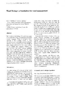
The guide "Principles of Weed Management" is a single text so does not lend itself to database storage. The encyclopaedia also displays information from the ArableDS data sharing environment (Parsons et al, 2005). Data storage and use The data were stored in an Access database. In addition to storing the collected data. each item has its source identified for traceability, attribution and validation. Information was stored with the removal of as much technical language as possible. Storage and flow of encyclopaedic data is shown in figure 1.
Data Sharing Environment Weed Manager
Pesticide data
Herbicide label information Herbicide & cultivation effect data
Herbicide encyclopaedia
Weed information
Weed names
Images Weed searches Environmental searches Principles of weed biology /Wrag guidelines
Discursive HTML pages
Weed descriptive information Weed Biology, Geography Agriculture Icons and Search queries Graphic Paths
Weed Manager Module
Pages
Key Database driven Combination Static
Data Infrequently updated Frequently updated Files stored on hard drive
Figure 1: Storage and flow of information in Weed Manager and the ArableDSE. There are two types of encyclopaedic data available; that used both by the Weed Manager modules (dotted lines) and the encyclopaedia (solid lines), and information only used in the encyclopaedia. Some information feeds to one part of the encyclopaedia whereas other information is used by many parts of the system, for example, herbicide effect information feeds into both herbicide and weed information pages and also into the decision module. The shading on the databases indicates the updating requirements. Similarly, the shading on the pages indicates the nature of the pages. The weed information consists of over 60 different types of information such as descriptions, geographical locations and image files. In order to simplify data entry, validation and access, the data were split into separate tables with a common key. The key selected was the Eppo Code which is a five letter unique identifier of every vascular plant derived from the scientific name. The Eppo Code was used in the naming of all images simplifying the development of the encyclopaedia, and image source links. Information display The data stored in the database can be displayed in three ways; directly from the database; pages generated in advance, or a combination of the two methods. In all cases there is a balance to be struck.
61
Pages which are drawn dynamically (straight from the database) have a significant time penalty on loading, but require only one file change for updating. Pages that are stored as individual files will have an increased size for storage compared with the information stored only in the database but will load more quickly. Table 1 shows the page type and reason for choosing this for each part of the encyclopaedia. Table 1: Encyclopaedic parts of the encyclopaedia. Part of encyclopaedia Type of page Herbicide information Directly from database Weed information
Combination
Weed identification searches Directly from database Principles of weed Static stand-alone pages management Environmental searches Directly from database
reason Frequently updated + data used in the module includes weed - herbicide interactions which are frequently updated + data used in the module Requires interactive queries Essay style information Requires interactive queries
The pages with content drawn directly from the database use a specifically written component which isolates the files from the database, so that pages do not have to be rewritten if the database structure, information or the location changes. User interface design Simple rules were used in the design of the encyclopaedic interface: 1. Sections and pages should be easily navigated. 2. The section of the encyclopaedia being viewed should be clear (obvious location). 3. Users should see as much information as possible without scrolling at 600*800 resolution and with minimal use of the mouse. Navigation The ArableDS browser displays an index so that navigation to any section of the encyclopaedia is simple. Links between pages and section are available as tabs or buttons on each page. Location The basic division of the encyclopaedia into product-related and weed-related information is marked by a change in livery, controlled by external stylesheets. Information display Information is presented in a card index format with almost all information visible on each card to reduce the need for scrolling,. Each card tab activates layers in the page to display relevant information and photographs. I have removed " " for consistency - if included should be single quotes ''. Some information is common to both the weed and herbicide pages and is displayed in the same way to help users navigate. For example, the information relating to the effect of herbicides and cultivations on weeds, which is used in the decision module, comes from the database and is displayed in both the herbicide and weed information pages in a similar format with colour coding used for emphasis. Extra herbicide efficacy information which has been collected for encyclopaedic use from papers and independent trials is displayed separately, but in the same format.
62
Implementation The basic structure of each page type is simple HTML using javascript to hide and display page layers, and modify page information. When a page is loaded, all the information for that page is present, but only the most important is displayed with the rest on hidden layers.
Herbicide information The herbicide encyclopaedia is fully database driven. There is only one file which allows a user to select herbicides. The data for the selected herbicide then populates the page. Users requested that the 10 most useful items of information should be immediately visible (Park, Parker and Ginsburg, 2004); these are displayed on the top layer. Hidden layers can be accessed at the click of a button.
Figure 2: Picture of the herbicide encyclopaedic page Weed information Weed biology information combines information generated in advance with database driven sections. Each weed has a separate file in index card format. Hidden layers are accessed by clicking the card index tabs. The herbicide and cultivation effects information are displayed in a pop-up window. A dialog application was written to create static pages from a database. A template page was developed specifying the format of the new file, the location of the populating data in the database and the javascript required to display the herbicide effect information from the database and control the page dynamics. The output is a series of files, one for each Eppo code in the database. It was not possible to remove all the technical language from the encyclopaedia so some explanation is necessary. Two mechanisms are used to provide these explanations. For each weed information page, tool tip style explanations are added to words and phrases in the encyclopaedia. A second dialog application was written to add tool tips to selected words and phrases in the html files. This allows the definitions to be stored separately from the basic data in a database table. The program searches for each glossary item in the text of a file and replaces the item with the required html and definition. All the terminology is also listed on a single glossary page
63
Figure 3: Picture of weed biology page Weed identification searches Weed searches presented a new design problem. There are various available keys for plants and weeds with common identification systems, which divide weeds into different classes and identify them by this class (i.e. Chancellor; 66, Hanf, 83). The botanical keys used in printed botanical guides usually identify plants by flower although some include mature plant stages, agricultural guides show early plant growth stages at which time weeds are usually controlled. Where keys are language based, botanical terms are often used, increasing the difficulty for non botanists.. Traditionally, users may have to make from 5- 20 decisions to identify the plant. In most botanical keys, one pathway through the key leads to the plant in question but this does not take user error into account. As a result they may discard the key, and instead skim through every possible picture before they recognise the plant. Electronic identification keys can have a "many to one" relationship, where, for example a cotyledon can be a member of several different sets of characters. (Figure 3).
Notched cleavers
Oblong
hemp nettle
field bindweed
prickly sowthistle
Round or wide Figure 3. A leaf can be characterised by one or many sets, choosing one of the sets defined in Weed Manager will retrieve all the members of that set., even if they belong to other sets.
64
The number of options that can be displayed on a screen is limited and the users preferred fewer choices. The Weed Manager identification keys were designed to minimise the number of decisions and allow for overlapping sets. The first decisions, the type of weed (grass or broad-leaved), and the growth stage (young or flowering), have mutually exclusive classes and are made by clicking on the index card tabs which call the appropriate search interface page. Each page is populated with simple radio button or check box choices with a maximum of 7 categories (sets) from which to choose. These pages are database driven because they display the results of queries. The results are displayed as thumbnails, which link to the weed information pages. Insert figure Figure 4: The search page for young broad-leaved weeds A simple guide to weed management The Principles of Weed Management includes background information on weed biology, soils, weed control in conventional and organic systems, and access to the WRAG guidelines (herbicide resistance management), and biodiversity. There are guides to growth stages of wheat, grasses and broad-leaved weeds, and pictures showing the number of weeds which give 5% yield loss in winter wheat. This was included to increase the users' confidence in the data they were entering into the mathematical modules which leads to greater confidence in the output. Each section of the principles is a single static file. Insert figure Figure 5: The simple guide to weed management Environmental searches Weed Manager contains a search to enable users to find weeds with particular environmental characteristics such as support for farmland birds (a prime environmental indicator), butterflies and rarity. This was a late requirement so was developed as a static page, but it should be converted to a database driven page in the future. This information is also displayed as icons in the decision module and weed information pages. The Environmental search page uses select controls to output lists of non-crop plants in any particular environmental category, with links to the relevant weed information page. Insert figure Figure 6: An environmental search User feedback Weed Manager was reviewed by users in 2004 (HGCA reference). Users were very positive about the design of the encyclopaedia and found it intuitive and easy to find the information they required. The encyclopaedia and the module are seen as complementary sources for information on weed control.
65
Conclusion Although the Weed Manager encyclopaedia has met the defined user needs, it is still being reviewed and updated to reflect changing needs and interface problems. Developers continuously monitor user-feedback for incorporation into future editions. The database driven pages are slow to load, at present this is met by showing the proportion of information gathered with a progress bar. While reducing worry about loading, this does however slightly increase page loading time. Further work needs to be done to speed up these pages. The security patch update for windows XP has also presented problems to naïve users, by blocking the dynamic pop up windows. The solution to this problem will require some design changes. References Chancellor, R.J., The identification of weed seedlings of farm and garden, 1966, Blackwell Scientific Publications Hanf, M. 1983, The Arable Weeds of Europe with their seedlings and seeds, 1983, BASF Park, C., Parker, C., and Ginsberg, D., Workshops as a cost-effective way to gather requirements and test user interface usability? Findings from WMSS, a decision support developemnt project., 2004, Contemporary Ergonomics Parker, C. G. and Clarke, J. H., Weed Management: Supporting Better Decisions., 2001, Proceedings of the BCPC conference - Weeds 2001 Parker, C., G., Decision Support Systems: Lessons from past failures, 1999, Farm Management, 10 (5), , 273-289, Parsons, D., A. Mayes, Meakin, P. A. Offer, and Paveley, N., Taking DESSAC forward with the Arable Decision Support Community., 2004, Aspects of Applied Biology
66
APPENDIX D (Draft paper version 3 on 02/12/05)
A model to simulate the growth, development and competitive effect of weeds in a winter wheat crop in the United Kingdom. L. R. Benjamin, P J Lutman, J. Cussans, J. Storkey Introduction The decision whether to control weeds, and what weed control measure to choose, is often a complex trade-off between likely economic impact of the weeds at the density and size present, the cost of weed control measure and the efficacy of the weed control measures, given the growth stage of the weeds. Many attempts have been made to attempt to quantify this trade-off by developing growth, development and competition models. Simple empirical relationships relating crop yield loss to weed density has been developed (Cousens, 1985) and this has been developed to relate yield loss to the early relative leaf areas of weeds and the crop (van Acker et al., 1997). More complex ecophysiological models have been developed, which are able to take a more mechanistic approach to simulating weed – crop competition (Kropff and van Laar, 1993). Several decision support systems for weed control have been developed from these models, for example (Hoffman et al., 1999) (need to check this paper, I do not have a reprint!!). The effects of tillage on Amaranthus species seedling emergence have been simulated with the intention of incorporating the emergence models within ecophysiological growth and competition models for decisions on weed control (Oryokot et al., 1997). A decision support system (WHEATMAN) for was developed to take account of the specific conditions for Australian wheat growers (Woodruff, 1992). In this model, weed infestation was only one of several environmental factors affecting wheat productivity. A GIS-based decision support software has been developed to aid weed control in developing countries (Zesheng and Ling, 1997). This approach included a database of herbicide activities and dose-response curves for various weed species. The decision support software produced a herbicide spray map. Weed management decision models have been perceived as having mainly an educational value rather than as a tool for making specific strategic or tactical decisions (Wilkerson et al., 2002). Decision support software may be perceived as too simple; not taking into account all the factors that influence the interaction between crop and weed, or ignoring all the factors that growers need to consider in crop husbandry. Decision support can also be considered too complex, requiring information that is difficult or impossible to obtain in commercial practice (Wilkerson et al., 2002). To date, no decision support software has been developed for crops grown in the United Kingdom. In this paper the models that lie behind a new decision support system, WMSS are described. WMSS is a Weed Management Support System, intended to support strategic decision for weed control in winter wheat crops in the United Kingdom. This paper deals with the methodology of the biological models that simulate weed and crop growth within a growing season. A complementary paper will describe the population dynamics of weed species through a crop rotation which includes winter wheat crops. The models described in the paper have been calibrated for the following weeds; black-grass, chickweed, cleavers, wild oat, barren brome, Italian ryegrass, annual meadow grass, fat hen, poppy and knotgrass. Also, the following two crops that act as volunteer weeds were parameterised; winter oilseed rape and field beans. WMSS is part of the suite of models that take advantage of the DESSAC platform. This allows the advantage that many features of a site, such as soil type, meteorological data, and features of herbicides, and be accessed from the DESSAC platform. Description of the Within Season Model Climate and Astronomical Data Calculation of day length is based on time of year and latitude, using the ASTRO procedure (Kropff and van Laar, 1993). The duration of the photoperiod was calculated as for day length, but assumed that the start and end were determined when the sun was 6 degrees below the horizon.
67
Maximum and minimum temperatures, radiation, rainfall, evapotranspiration from a reference crop were collated from a range of sites across the United Kingdom ((Parsons et al., 2004)). For any one site and season these data records were retrieved from 1st of January of year of drilling to 31st December of the year of harvest. Daily day degrees were calculated based on integrating the area above the base and a diurnal sine curved around the maximum and minimum temperatures (refer to appendix to write out full set of equations). Seedling establishment Seasonality of Emergence and Soil Water For most weed species seedling establishment is confined to periods of the year, even when temperature and soil moisture are adequate for establishment at other times of the year. This seasonality of establishment has been described for several weed species by (Roberts and Feast, 1973). The numbers of seedlings established in each month of the year was read off the graphs of seasonality and tables of establishment for A. myosuroides, Avena fatua, Chenpodium album, G. aparine, Matricaria matricoides, Papaver rhoeas, Poa annua, Polygonum aviculare and S. media from the Weed Control Handbook (1990), for Capsella bursa-pastoris, Euphorbia helioscopia, Fumaria officinalis, Fallopia convolvulus, and Veronica hederifolia from (Roberts and Feast, 1973) and Anisantha sterilis from (Froud-Williams, 1983). For each species, the numbers establishing each month were expressed as a proportion of the maximum number of seedlings emerging in the year. These numbers of seedlings emerging on any one day are a function of the dormancy of the seeds and the soil water and temperature regime. To quantify the extent of seed dormancy, it was necessary to allow for any effects that soil moisture and temperature may have had on the seasonal emergence patterns reported by (1990; Froud-Williams, 1983; Roberts and Feast, 1973). The influence of soil moisture on seasonal emergence was assumed to have been obscured by the use of data from several years. Although soil moisture is likely to be lower in summer, sporadic rainfall may produce periods in the summer when soil moisture is higher than in some periods in the winter. Hence, it was assumed that soil moisture had a negligible effect on the seasonal emergence patterns reported. Although there are sporadic fluctuations in temperature throughout the year, the soil temperature in summer can be assumed to be never lower than that in winter. A means of adjusting the reported seasonal emergence patterns for soil temperature was sought by examining the seasonal emergence of P. annua, which has no dormancy. Hence, for this species, the difference between numbers emerging in different months could be attributed entirely to soil temperature. More explicitly, for each month, the ratio of emergence of P. annua in July (the month with the greatest emergence) to the monthly emergence was taken as a weighting factor to apply to the monthly emergence of each other weed species, to render the emergence pattern independent of soil temperature. For each weed species, the numbers emerging each month were adjusted by the P. annua weighting factor, and these numbers summed for all twelve months of the year. The numbers emerging in each month were then scaled as a proportion of the total numbers emerging over the entire year. The accumulated scaled and P. annua adjusted monthly emergence values for each species were calculated, n. A cubic polynomial fitted was fitted to n for each species. Hence, nt = a + b.t + c.t 2 + d .t 3 1 where t is the day of the year. The rate in change in the value of n is a measure the daily dormancy value of the species. That is, where the change in cumulative numbers of seedlings appearing is great, then the dormancy must be low, whereas where the cumulative numbers remains constant with time, then dormancy must be high.
68
By differentiating eqn 5, the rate of change in cumulative numbers,
dnt
dt
= b + 2.c.t + 3.d .t 2
The value of
dnt
dt
dnt
dt
, is given by 2
was calculated as a proportion, S, of the maximum value of
dnt
dt
, so that on
any day the value S varied between 0 and 1. The value of S was used in eqn 3 to calculate the value of Dm. Temperature-Driven Seedling Emergence For the each species, the accumulated number of seedlings emerged, n, at any site s on day t is described by a logistic equation, based on thermal time.
n s, t = A + C s /(1 + exp(-B.(Xt - M)))
3 where Xt is the accumulated day degrees, modified by the seasonality and moisture limitation, above a base temperature Tb from the sowing date to day t. A is a number of seedlings present at Xt=0, and A + C is the maximum number of seedlings to establish, and varies between sites and years. M is the duration to the inflexion point of the logistic curve and B is the slope of the curve at the inflexion point. The seedling emergence counts used for fitting eqn 3 were for winter wheat (Triticum aestivium), black-grass (Alopecurus myosuroides), cleavers (Galium aparine), and chickweed (Stellaria media), recorded at six sites in the England in one year and five of these sites in the subsequent two years, giving a total of 16 site/year combinations (Ingle et al., 1997). Differences between species in observed seedling emergence patterns were not great (Table 1, Figures 1, 2, 3 and 4). Wheat was the fastest species to emerge with a mean emergence date of 33 days after sowing, with a range of 8 to 89 days. Cleavers was the slowest with a mean emergence date of 40 days with a range of 14 to 98 days. Initially when fitting eqn 3, A, C, B, M and Tb were determined by fitting eqn 3 to seedling emergence counts using a Nelder – Mead unconstrained minimisation procedure, called FMINSEARCH (Matlab, 1996). The estimated values of Tb were often unreasonable low (of the order of -40oC), and it was concluded that the range of temperatures during the experimental period were not sufficiently broad to allow this parameter to be estimated accurately from the data. Consequently, the value of Tb was set at 0oC and the dormancy modified day degrees for each species were calculated from sowing to each of the seedling counts. Eqn 3, was fitted to each species separately using the FITCURVE directive of Genstat (Genstat, 2002). First of all, with the value of Tb fixed at 0, and the accumulated effective day degrees for each of the species was calculated from crop sowing each of the seedling emergence recording dates. For each species common values of B and M (Table 2) were estimated over all the datasets, but A and C were allowed to vary with site – year combination. The agreement between observed and fitted data was generally close (Figs 1, 2, 3 and 4). The fitted lines were sometimes not smooth because the driving variable for eqn 3 is day degrees modified by the dormancy, which varies with day of the year and species. The data in the figures are plotted against days after sowing, as this is more meaningful a scale than day degrees. It may seem odd that the value of M for wheat is greater than that for any of the weed species (Table 1). This is because given the dormancy that occurs within the species, there is no close linkage between chronological time and time on a day degrees basis. Within WMSS, emergence of winter wheat is simulated as a single cohort of seedlings emerging M day degrees after drilling. The density of seedlings in this cohort is taken as the average of the range specified by the user. The simulation of weed emergence with WMSS is more complex. Each weed species emerges as eight cohorts of seedlings. The number of seedlings in each cohort is calculated as an eighth of the average of the density range specified by the user. Furthermore, the accumulation of thermal time
69
for progression to germination and emergence is modified by daily soil moisture and seasonality of establishment factors. The stimulus for establishment is in reference to the date of drilling for one of the cohorts and to the date that the previous crop was harvested for the remaining seven cohorts. For the cohort whose establishment is in reference to drilling, germination occurs on the drilling date and establishment occurs after 80 modified day degrees have accumulated. For the other cohorts, the accumulated modified day degrees, Xˆ e , when a proportion f of the population has emerged can be obtained by re-arranging eqn 1.
Xˆ e = (M.B - log((1 - f)/f))/B
4
The values of Xˆ e that corresponds to values of f of 0.125, 0.250, 0.375, 0.500, 0.625, 0.75 and 0.875 were calculated, and assigned to the day degree requirement for emergence of cohorts one to seven, respectively. The germination requirement was calculated as Xˆ g = max[ Xˆ e − 80,0] for each cohort. The dates of seedling germination and emergence from either the drilling date or date of the previous harvest was determined when the accumulated modified day degrees exceeded the germination and emergence requirements, calculated from eqn 2. On each day, the day degrees, Dm, were calculated as
Dm = D.ψ .S
5 where D is the day degrees above a the base temperature (calculated based on a diurnal sine curve fluctuation between the maximum and minimum temperatures), ψ is a term for soil water content and S is a term for the seasonality of seedling establishment. It was assumed that the soil after harvest or drilling is initially dry and the value of ψ was set to 0. On each day, t, a running rainfall total, R, was calculated, with the total incremented by rainfall, r, and subtracted by evapotranspiration, E. The running total was not allowed to fall below zero or exceed 20 mm.
R t = Rt −1 + rt − Et Rt = max[ Rt ,0]
6
Rt = min[ Rt ,20] If Rt exceeded 5, then ψ was set to 1. Phenology For graminaceous weeds, the decimal code scale of development for cereals was adopted (Zadoks et al., 1974). The progression of development along the decimal code was based on thermal time modified by vernalisation and photoperiod effects. An accumulated photovernal thermal time (PVTT) was calculated for each cohort of each species (Milne et al., 2003). The Zadoks values for the plants from anthesis to maturity were identical to that of Milne et al. (2003), but their paper dealt only with the timing of appearance of culm leaves and ear maturity, because their model was targeted at disease control on the upper canopy. The model by Milne et al. (2003) used the timing of anthesis and the calculation of the phyllochron as a reference point for the production of the culm leaves. The phyllochron ρ, was related to the rate of change of day length by
70
ρ=
1 α + βR
7
where α and β are parameters, and R is the rate of change of day length on the day of plant emergence, te (with 1st January equal to 1). The value of R was approximated by
R=
10π (t − 444) cos 2π e 365 365
8
Growth stage 0 was achieved on the date of germination, and the growth stage, Z, on any date, t, from germination to emergence was given as i =t
∑D
i =t g
i
Z = 10. i = t e
9
∑D
i =t g
i
where D is day degrees. After emergence, the value of Z remains at 10 until the first leaf is formed. A new leaf was assumed appear when the accumulated day degrees from the appearance of the previous leaf had exceed the value of the phyllochron, ρ . On the appearance of a leaf, any difference between the accumulated day degrees and ρ was not lost, but contributed to the accumulation of day degrees for the appearance of the next leaf. The values of Z increased from 11, 12, 13 … 19 with the appearance of first, second, third … and ninth leaves, respectively on the entire plant. The value of Z remains at 19 when there were nine or more leaves present. In practice values of Z greater than 13 or 14 are never utilised, because once the tillers appear, the value of Z was increased from 21, 22, 23 … 29 with the appearance of first, second, third … and ninth tillers, respectively on the entire plant. The progress towards tillering is assumed to occur when a set number of phyllochrons, Φ , have been produced from emergence. Also, secondary and higher order tillers start to be produced once Φ phyllochrons have elapse since the initiation of the mother tiller. Tillers are produced once the accumulated thermal time exceeds the phyllochron for tillering, φT . The processes of leaf production, and tillering continue until main stem extension, Zadoks 30, which is calculated as a fixed number of phyllochrons before the time of anthesis (Milne et al., 2003). For broad-leaved weeds, a similar approach is taken. The calculation of germination and emergence time is identical in approach as that for graminaceous weeds. The subsequent growth stages are based solely on the number of leaves on the entire plant. Unlike graminaceous weeds, the equivalent of tillering (that is branching) does not directly affect the growth stage code. Branching, however, is simulated in an identical process to tillering, so that a correct number of leaves on the entire plant is estimated. One further difference is that the number of leaves produced per phyllochron may be more than one. For G. aparine, each whorl of leaves is treated as though it is a single leaf. Crop Yield Loss The estimation of crop yield loss is based on a mixture of a complex eco-physiological model and a simple empirical static yield loss equation. The underlying principle is to allow the entire community of plants to increment in green area to the point of canopy closure. The ratio of individual weed species green area to the sum of the crop and individual weed species leaf area is used to estimate the crop yield loss associated with that species. The growth of each species in the community from emergence to canopy closure is simulated using the ecophysiological model of (Kropff and van Laar, 1993). The initial green area index (GAI) of each cohort of the weed and that of the crop is based on the green area per seedling at the time of full hypocotyls or cotyledon expansion and the density of the cohort or of the crop.
71
Where this initial seedling green area is not known, then for grass species, the value is estimated as the product of the green area per black-grass seedling (0.000035 m2) and the ratio of the species seed weight to the seed weight of black-grass (1.1 mg). For broadleafed species, the initial green area is estimated as the product of the green area per chickweed seedling (0.000031 m2) and the ratio of the species seed weight to the seed weight of chickweed (1.1 mg). The simulation commences on the date of emergence of the first cohort of the weed or the crop (which ever is the earliest), and the simulation allows the inclusion of further weed cohorts as the simulation proceeds. The simulation ends when the GAI of the entire community equals 0.75, which is taken as the point of canopy closure. The yield loss associated with a species is calculated as
YL =
Y.q.Lw 1 + (q - 1).Lw
10
where Y is the crop yield in weed-free conditions, q is the damage coefficient constant specific to the combination of crop and weed species and Lw is given by
Lw =
GAI weed GAI weed + GAI crop
11
(Kropff et al., 1995). Note, that the value GAIweed is the GAI summed over all the cohorts of the weed species present at the time of canopy closure. The weeds are assumed to act independently of one another, but the summated yield losses were not allowed to exceed weed-free crop yield. This assumption removed the necessity to simulate weed-on-weed interactions. In most commercial conditions, weed densities are sufficiently low to render these interactions to be of no biological importance, although they can be considerable in experimental circumstances. Weed Control Measures Herbicides and mechanical cultivations are assumed to destroy the GAI of the weeds, with an efficacy that varies with weed species and weed growth stage. For the purposes of WMSS, grass weed growth stages were grouped into the following nine categories of Zadoks values, 0-7; 8-10; 1113; 14-21; 22-29; 30-31; 32-39; 40-45 and 46-93. Broadleafed weed growth stages were grouped into the following six categories, pre-emergence; cotyledons – two leaves; two – four leaves; four – six leaves; six leaves – eight leaves; more than eight leaves to flowering. Note that the flowering growth stage will take precedence over the vegetative growth stages if flowing occurs sooner than eight leaves. The proportion of GAI lost due to cultivations or herbicides (hereafter called ‘product’) was grouped according the following levels as, 0.00 for certain growth stages, where weeds are immune to weed control such as weed pre-germination; 0.01 for weeds resistant to a product, or a product of unknown efficacy; 0.51 for weeds moderately resistant to a product; 0.76 for weeds moderately sensitive to a product; 0.91 for weeds sensitive to a product; 1.00 for herbicidal sprays applied to emerged weeds pre-crop emergence. Each weed species, growth stage and product combination was assigned a level of proportional kill (D. H. K. Davis, personal communication). This level of control was assumed to be unaffected by the cohort number of the weed species. A programme of cultivations and sprays was considered by calculating the efficacy of each spray and cultivation. Let ξ s,i be the percentage control of cohort i of product s as determined by the growth stage of the cohort at the time of product application. Hence, the survival is given by 1 − ξ s,i . For a spray program of M products, then the combined survival of cohort i is given by the multiplicative s=M survival response model, ∏ s =1 (1 − ξ s ,i ) . The proportion of cohort i controlled, Ci, by the spray
72
s=M
program is given by 1 − ∏s =1 (1 − ξ s ,i ) . For the entire species, containing n cohorts, the percentage control, K, is given by i=n
K=
∑ Gi .Ci
i =1 i =n
.100
12
∑ Gi
i =1
where G is GAI at the time of canopy closure. Hence, a feature of WMSS, is to calculate the proportion of the erosion of GAI according to the growth stage of the weed at the time of the application of the product. The next assumption is that this erosion of GAI occurs at the time of canopy closure. This assumption may appear odd, but it has important implications for reducing the number of calculations, which is particularly important when different spray programmes are being compared by the optimisation model within WMSS. This assumption means that the complex dynamic ecophysiological model to calculate the species value for G need be run only once at the outset with a control cultivation programme that is sufficient only to establish the crop. Cultivations can stimulate the emergence of weed seedlings (Vleeshouwers and Kropff, 2000). This breakage of dormancy is due to complex physiological processes that have not yet been successfully simulated (Vleeshouwers and Kropff, 2000). In WMSS, an empirical approach is taken, in which the stimulation of weed emergence is handled relatively empirically, with the emergence date of cohort number seven being advance to emerge 80 modified day degrees after the first cultivation. In effect, the assumption within WMSS is that delay in emergence of cohort seven is due to a dormancy mechanism that is broken by soil disturbance. Ploughing is treated differently to other cultivations. This is because whereas other cultivations disturb the soil, ploughing inverts the soil profile. In effect, ploughing replaces the soil seedbank in the soil layer from which weed seedlings can establish with a new soil seedbank. WMSS assumes that the entire soil profile weed seedbank is so large that the new seedbank in the shallow layer after ploughing is just as great as the pre-ploughing one. The impact of ploughing id to delay the emergence of cohorts one to seven to be with reference to the date of ploughing rather than with reference to the date of the last harvest. Observations An important feature of WMSS, is that users can provide observations of the crop and/or weed, which will adjust the simulation results to current circumstances. Observations of growth stage, cover and density can be entered. Growth stage observations are handled by comparing the growth stage that the user is specifying for a weed on a date with the growth stage that is currently calculated for the most precocious cohort. The growth stages of all the cohorts is advanced or retarded by the difference in time between the observed and currently expected values. Wheareas WMSS deals with GAI, users are more likely to be able to observe percentage ground cover. Hence, the first action when dealing with a cover observation is to convert it to a GAI value. The simple conversion, GAI=0.0278.percentage ground cover. The equation is robust up to 5 percent ground cover (J. Storkey, personal communication). The procedure within WMSS is to calculate the ratio of the summed GAI for all cohorts of a species expected at the date of the observation to the GAI observed for the species. In calculating the expected GAI any potential reduction in GAI due to weed control measures are included in the simulation from emergence of the first cohort to the date of observation. The ratio of observed to expected GAI is used as a factor to multiply the green area per seedling at the time of emergence. 73
Hence, if the observed GAI is twice that which would be expected, then the entire wmss model is run gain with the GA at emergence being inflated by the discrepancy between emerged and expected GAI.
74
Table 1. The difference between the expected and observed days after sowing to achieve the observed numbers of seedlings
Wheat mean observed days after sowing first observed day after sowing last observed day after sowing
32.9
Species Black-grass Chickweed 34.3
34.5
Cleavers 39.5
8
10
9
14
89
89
98
98
75
Table 2. Value of parameters B and M from eqn (1) for wheat, black-grass, chickweed and cleavers, fitted to the seedling emergence data from (Ingle et al., 1997) ± standard error.
Wheat Parameter B (oC-1) M (oC) number
0.0174±0.00280 159±9.4 138
Black-grass
Species Chickweed
0.0261±0.00388 112±3.9 150
76
0.0263±0.00293 103±4.0 144
Cleavers
0.0228±0.00252 142±6.9 156
LITERATURE CITED 1990. Weed control handbook: principles. Blackwell Scientific Publications, Oxford, UK 8. Cousens, R. 1985. A simple model relating yield loss to weed density. Annals of Applied Biology 107:239-252. Froud-Williams, R.J. 1983. The influence of straw disposal and cultivation regime on the population dynamics of Bromus sterilis. Annals of Applied Biology 103:139-148. Genstat. 2002. Genstat, 6th Edition VSN International Ltd, Hemel Hempstead, United Kingdom. Hoffman, M.L., D.D. Buhler, and M.D.K. Owen. 1999. Weed population and crop yield response to recommendations from a weed control decision aid. Agronomy Journal 91:386-392. Ingle, S., A.M. Blair, and J.W. Cussans. 1997. The use of weed density to predict winter wheat yield. Aspects of Applied Biology 50:393-400. Kropff, M.J., and H.H. van Laar. 1993. Modelling crop-weed interactions CAB International, Wallingford, UK. Kropff, M.J., L.A.P. Lotz, S.E. Weaver, H.J. Bos, J. Wallinga, and T. Migo. 1995. A two parameter model for prediction of crop loss by weed competition from early observations of relative leaf area of the weeds. Annals of Applied Biology 126:329-346. Matlab. 1996. The Matworks Inc., Nantick, Massachussetts, USA. Milne, A., N. Paveley, E. Audsley, and P. Livermore. 2003. A Wheat Canopy Model For Use In Disease Management Decision Support Systems. Annals of Applied Biology in press. Oryokot, J.O.E., L.A. Hunt, S. Murphy, and C.J. Swanton. 1997. Simulation of pigweed (Amaranthus spp.) seedling emergence in different tillage systems. Weed Science 45:684690. Parsons, D., A. Mayes, P. Meakin, A. Offer, and N. Paveley. 2004. Taking DESSAC forward with the Arable Decision Support Community. Aspects of Applied Biology submitted. Roberts, H.A., and P.M. Feast. 1973. Weeds in cultivated and undisturbed soil. Journal of Applied Ecology 10:133-143. van Acker, R.C., P.J.W. Lutman, and R.J. Froud-Williams. 1997. Predicting yield loss due to interference from two weed species using early observations of relative weed leaf area. Weed Research (Oxford) 37:287-299. Vleeshouwers, L.M., and M.J. Kropff. 2000. Modelling field emergence patterns in arable weeds. New Phytologist 148:445-457. Wilkerson, G.G., L.J. Wiles, and A.B. Bennett. 2002. Weed management decision models: pitfalls, perceptions, and possibilities of the economic threshold approach. Weed Science 50:411424. Woodruff, D.R. 1992. 'Wheatman' a decision support system for wheat management in subtropical Australia. Australian Journal of Agricultural Research 43:1483-1499. Zadoks, J.C., T.T. Chang, and C.F. Konzak. 1974. A decimal code for the growth stages of cereals. Weed Research 14:415-421. (ed.) 1997. 1997 ESRI user conference.
77
Legend For Figures
Figure 1. The relationship between number of black-grass seedlings emerged and days after sowing of (a) Boxworth, (b) Bridgets, (c) Drayton, (d) High Mowthorpe, (e) Rothamsted and (f) Woburn (Ingle et al., 1997). Symbols are the observed counts and the lines fitted by Eqn (3) with common values of B and M but different values of C and A between years and sites. Circles and solid line for 1994-5, squares and dashed line for 1995-6 and triangles and dotted line for 1996-7. Figure 2. The relationship between number of chickweed seedlings emerged and days after sowing of (a) Boxworth, (b) Bridgets, (c) Drayton, (d) High Mowthorpe, (e) Rothamsted and (f) Woburn (Ingle et al., 1997). Symbols are the observed counts and the lines fitted by Eqn (3) with common values of B and M but different values of C and A between years and sites. Circles and solid line for 1994-5, squares and dashed line for 1995-6 and triangles and dotted line for 1996-7. Figure 3. The relationship between number of cleavers seedlings emerged and days after sowing of (a) Boxworth, (b) Bridgets, (c) Drayton, (d) High Mowthorpe, (e) Rothamsted and (f) Woburn (Ingle et al., 1997). Symbols are the observed counts and the lines fitted by Eqn (3) with common values of B and M but different values of C and A between years and sites. Circles and solid line for 1994-5, squares and dashed line for 1995-6 and triangles and dotted line for 1996-7. Figure 4. The relationship between number of wheat seedlings emerged and days after sowing of (a) Boxworth, (b) Bridgets, (c) Drayton, (d) High Mowthorpe, (e) Rothamsted and (f) Woburn (Ingle et al., 1997). Symbols are the observed counts and the lines fitted by Eqn (3) with common values of B and M but different values of C and A between years and sites. Circles and solid line for 1994-5, squares and dashed line for 1995-6 and triangles and dotted line for 1996-7.
78
Fig. 1 a)
b)
350
400
300 300 Numbers (m-2)
Numbers (m-2)
250 200 150 100
200
100
50 0
0 0
20
60
80
Days After Sowing
c) 600
300
500
250
400
200
300 200
20
40
60
80
100
Days After Sowing
150 100
100 0
0
d)
Numbers (m-2)
Numbers (m-2)
40
50
0
20
40
60
80
0
100
Days After Sowing
e)
0
20
60
80
100
120
Days After Sowing
f)
500
40
350 300
400 Numbers (m-2)
Numbers (m-2)
250 300 200
200 150 100
100 0
50 0
10
20
30
40
0
50
Days After Sowing
0
10
20
30
Days After Sowing
79
40
50
Fig. 2 a)
b)
500
300 250 Numbers (m-2)
Numbers (m-2)
400 300 200 100 0
150 100 50 0
0
20
40
60
80
Days After Sowing
c)
600
300
500 Numbers (m-2)
200 150 100
20
40
60
80
100
Days After Sowing
400 300 200 100
50 0
0
d)
350
250 Numbers (m-2)
200
0
20
40
60
80
0
100
Days After Sowing
e)
0
20
60
80
100
120
Days After Sowing
f)
600
40
400
500 Numbers (m-2)
Numbers (m-2)
300 400 300 200
200
100 100 0
0
10
20
30
40
50
0
0
10
Days After Sowing
20
30
Days After Sowing
80
40
50
a)
b)
80
80
60
60 Numbers (m-2)
Numbers (m-2)
Fig. 3
40
20
20
0
0 0
20
60
80
120
100
100
80
80
60 40 20 0
20
40
60
80
100
Days After Sowing
60 40 20
0
20
40
60
80
0
100
Days After Sowing
e)
0
20
40
60
80
100
120
60
70
Days After Sowing
f)
120
50
100
40 Numbers (m-2)
80 60 40
30 20 10
20 0
0
d)
120
Numbers (m-2)
Numbers (m-2)
40 Days After Sowing
c)
Numbers (m-2)
40
0
10
20
30
40
50
60
0
0
10
Days After Sowing
20
30
40
50
Days After Sowing
81
a)
b)
500
500
400
400 Numbers (m-2)
Numbers (m-2)
Fig. 4
300 200
0 0
20
60
80
500
400
400
300 200 100 0
20
40
60
80
100
Days After Sowing
300 200 100
0
20
40
60
80
0
100
Days After Sowing
e)
0
20
40
60
80
100
120
Days After Sowing
f)
500
400
400 Numbers (m-2)
300
300 200
200
100
100 0
0
d)
500
Numbers (m-2)
Numbers (m-2)
40 Days After Sowing
c)
Numbers (m-2)
200 100
100 0
300
0
10
20
30
40
50
0
0
10
Days After Sowing
20
30
Days After Sowing
82
40
50
APPENDIX E Draft paper on 05/12/05
Modelling weed management over a rotation in the UK using stochastic dynamic programming L R BENJAMIN*, A E MILNE*, P J W LUTMAN*, J CUSSANS*, J STORKEY* & D J PARSONS† *
†
Rothamsted Research, Harpenden, Hertfordshire, AL5 2JQ, UK, and Cranfield University, Silsoe, Bedfordshire, MK45 4DT, UK
Short title: modelling weed management over a rotation Correspondence: L R Benjamin, Rothamsted Research, Harpenden, Hertfordshire, AL5 2JQ, UK. Tel: (+44) 1582 763133; Fax: (+44) 1582 760981; Email:
[email protected] Introduction
Weed control in UK arable crops is an expensive necessity for all arable farmers. The survey of pesticide usage in Great Britain in 2002 shows that on average herbicides were applied to wheat on 2.8 occasions, included 4.3 products and 5.3 active ingredients. Adequate weed control can often be achieved by tackling the problem as it occurs in the season of production. This is not necessarily the most cost effective approach, and as species become increasingly resistant to herbicides, it may not always be effective. An approach to weed control based on consideration of crop rotations is therefore likely to be more successful in the long term. By carefully planning the future rotation and cultivations, the weed seedbank, which controls the weed infestation level in the crop can be kept to a manageable level. Although a number of groups have developed models that endeavour to advise on within season weed control (Berti et al., 2003; Neeser et al., 2004; Bennett et al., 2003), much less attention has been paid to rotational weed management. The model presented here simulates changes in weed seedbank density (seeds m-2) from season to season given crop, sowing time, cultivation and herbicide control. Yield loss due to weeds is estimated in each season, and the associated margin calculated. This allows the effect of control strategies to be assessed in both terms of seedbank density and margin. Once the model is constructed, one is still faced with the question – given a certain size seedbank, what sequence of actions will give the best long term profit? The answer to this may not be straight-forward because controlling a weed in the current season may not give immediate financial reward, but could help avert uncontrollably high weed densities in a future season. The stochastic dynamic programming method (Howard, 1960) is ideally suited to solve problems of this type. It analyses a system and evaluates a strategy for each system state to maximise future rewards. In the case discussed here, the system is the weed population dynamic model, the system state is the seedbank density (seeds m-2), the strategy specifies crop, sowing time, cultivation and herbicide choice, and the reward is made up of future profit margins. 83
The model and dynamic programme were developed as part of a ‘rotational’ module within a decision support system for weed control in the UK (Collings et al., 2003). This decision support system is called Weed Manager (formerly Weed Managment Support System or WMSS) and it would be run on a personnel computer. Weed Manager is currently being parameterised for 12 common annual weed species, and was designed so that the user selects a subset of weed species that are most important in the selected field. They can then choose either to run the model for a 6 year time period choosing their own crop, sowing time, cultivation and herbicide control settings in each season, or ask the system to suggest a forward plan which gives the best profit margin. In both cases, the system presents the result of the actions both in terms of changing seedbank population and in terms of profit margin. Weed Manager is designed so that this rotational module runs alongside a ‘within season’ module that estimates in some detail the yield losses caused to winter wheat in any one growing season by alternative cultural and chemical management tools. The rotational module is based on the life cycle model developed by Moss (1990) for Alopecurus myosuroides Huds (black-grass), but can be applied to many annual plant species. In essence, it is based on estimation of seed fecundity and survival. Similar models have been proposed by Doyle et al. (1986) and Cousens et al. (1986) to describe the life cycle of A. myosuroides and Avena fatua L. (wild oats) respectively. These consider the soil to have a deep and shallow layer, and they track the changes in the seedbank in each layer. Seeds migrate between layers when cultivations are applied. Seedlings emerge from the shallow soil depth and are killed to variable degrees by the weed control practices. Surviving plants produce seeds that are returned to the soil seedbank in the shallow layer. These two state variables (shallow and deep seedbank) drive the change in the weed population through the rotation as modified by a series of management influenced parameters. Because of the large uncertainties present in many of the steps outlined above, it is necessary to describe them by probability distributions, leading to a stochastic model. Sells (1993, 1995) modified these later two models for use in a stochastic dynamic programme (Howard, 1960) which calculated the optimal strategy for controlling A. fatua and A. myosuroides. Because the memory requirements for a dynamic programme increase exponentially with the number of state variables (“the curse of dimensionality”) it was necessary to simplify the model to contain a single soil layer only. For the present system, it was decided that it was essential to include two layers (shallow and deep), so that the impact of alternative cultural practices on seed distribution in the soil could be modelled. By using slightly fewer discrete states for the seedbank in each layer than Sells, and given the increases in computing power available, it was found to be possible to solve a two-layer model for up to two weed species in an acceptable time. The method used to handle larger numbers of species will be discussed below.
84
Materials and methods The Dynamic Program Formulation
The formulation of the stochastic dynamic program is N f t (i ) = max ∑ pijk ( Rijk + λf t +1 ( j )) (1) k j =1 where ft(i) is the optimal expected financial reward for years t and beyond given that the system state is i at the beginning of year t. In this application the system state describes the number of seeds in the seedbank. The transition probability of going from state i to j given a strategy k is denoted pijk . The strategy describes a set of actions under which the system is
run. Here the strategy defines the crop, cultivation, sowing time and herbicide control. Rijk is the financial reward associated with going from state i to state j given strategy k, and λ is a discount factor which scales future expected rewards. The discount factor is 1+ I (2) λ= 1+ Ω where I is the current rate of inflation, here assumed to be 3%, and Ω is the interest rate, here assumed to be 6 %, giving λ the value 0.9717.
The solution of Equation 1 consists of a set of decision rules that describe the actions that should be followed given the state at the beginning of year t. Collectively, these rules form a strategy (usually known as policy in dynamic programming literature) for weed control throughout the rotation. The equation can be solved either to find a finite horizon solution or the infinite horizon solution (steady state solution). It is not always possible to find the infinite horizon solution either because the system does not satisfy the necessary conditions for the existence of a solution or because the problem does not converge within a reasonable time. For reasons discussed later, the model described here is solved as a finite horizon problem. Defining the state variable
To use a stochastic dynamic programme, the state variable (the weed seedbank density in each layer, seeds m-2) needs to be composed of discrete states. This is achieved by dividing the seedbank density into ranges. Sells (1993) divided the seedbank density into bands that increase in a geometrical progression, because of the exponential nature of weed population growth. A similar approach is taken in Weed Manager, but the bands used are related to the plant density bands used elsewhere in the system. As the relationships are dependent on the transition probabilities, and are also used when setting the initial states, the details will be described in a later section. For each layer there are six bands: [Ll(i-1), Ll(i)), i = 1,...,6; l = s (shallow) or d (deep) For a single weed species in the dynamic programme, the state of the system is thus described by a pair of index values (is , id ), where is is the shallow seedbank index and id is the deep seedbank index. If n weed species are considered at the same time, the state of the system is therefore described by 2n index values. Each combination of these index values is
85
a single state in the dynamic programming formulation, so the total number of states increases exponentially with the number of weeds. The seedbank dynamic model
The seedbank dynamic model describes the effect of a strategy on the weed seedbank. The starting point of the annual life cycle is taken, for convenience, shortly after the harvest of the crop. At this time, the entire weed population of each species is present only as a seedbank. The numbers of seeds (seeds m-2) in the shallow and deep layers at the start of year t are denoted by Ns (t) and Nd (t) respectively. The shallow layer is defined as the top 5 cm and the deep layer as between 5 and 25cm, the latter being the average depth of ploughing in the UK. When soil is then cultivated, a proportion d of the seeds in the shallow layer are buried to the deep layer and a proportion u of the seeds in the deep layer are brought up to the shallow layer. A proportion g of the seeds in the shallow layer then germinate (seedling establishment is possible only from seeds in the shallow layer). Herbicides are then applied with a proportion 1– θ of the seedlings surviving to become mature plants. The number of mature plants in year t is therefore N m (t ) = [N s (t )(1 − d ) + N d (t )u ]g (1 − θ ) (3) The number of viable seeds produced by the mature plants is N (t )(1 − l )vhβ S (t ) = m (4) 1 + αN m (t ) where α and β are constants relating plant density to fruit production, v is the proportion of seeds that are viable, l is the proportion of seeds lost by herbivory and h is the number of seeds per fruit (note, h for some weed species is 1). If m is the proportion of ungerminated seeds that die in the soil per year. Then the number of viable seeds that persist in the shallow layer during year t is Q(t ) = [N s (t )(1 − d ) + N d (t )u ](1 − g )(1 − m) (5) Therefore the number of seeds in the shallow layer at the beginning of year t+1 is N s (t + 1) = S (t ) + Q(t ) (6) There is no direct contribution of seed rain to the deep seed layer at the start of each year. Hence the number of seeds in the deep layer at the beginning of year t+1 is N d (t + 1) = [N s (t )d + N d (t )(1 − u )](1 − m) (7) Season of drilling
The rotational model augments the kill of seedlings, θ, from mechanical and herbicide weed control measures, with the loss of weed seedlings due to delayed drilling. This is done by using the seasonal emergence patterns of the weed species Mortimer (1990), that were described by a cubic polynomial relation between accumulative seedling emergence and day of the year (Benjamin et al., 2005) . The proportion of kill due to delayed drilling was assumed to be the ratio number of seedlings that emerged before drilling to the total number of seedlings to emerge.
86
An earliest possible seedbed preparation date was defined for each crop, based on expert opinion. The period of total seedling emergence was assumed to be from this earliest sowing date to 60 days after this date, or, for spring-sown crops, from the 1st August of the previous year to 60 days after the earliest sown date. The period for emergence for seedlings that emerge before drilling is from the earliest sowing date to the date of drilling, or, for springsown crops, from the 1st August of the previous year to the date of drilling. The amount of emergence on each day was calculated by differentiating the cubic polynomial equation in Benjamin et al. (2005). This value was not allowed to be negative, which can occur with cubic polynomials. The more simple approach of differencing the values of emergence at two dates from the undifferentiated cubic polynomial was not taken because the slopes of the curve could be negative. Calculating the transition probabilities
The stochastic dynamic programme requires the probabilities associated with going from a known state i in year t to each of the possible states in year t + 1 for a defined strategy. Ideally each of the model parameter values should be described by a probability distribution, as this reflects the natural processes occurring. However, it is not always practical to assign a distribution to each of the parameters, either because of lack of appropriate data or because the calculations are computationally too time consuming. Sells (1993) considered only the effect of the herbicide application to be uncertain in her models as this had the largest effect on future seedbank. She considered the effects of five commercial herbicides for which she had data, but because of the way herbicide effects are included here, no similar data are available for Weed Manager (see section on ‘The strategy’ below). For simplicity, the uncertainty in seed numbers is solely attributed to the uncertainty of the starting state. When considering only a single weed species, the initial state is defined by [is id ]. To estimate the probability of ending up in shallow layer state js , first the lowest and highest seedbank densities that can occur in year t + 1 for a given strategy are calculated. To do this, equations 3–6 are used. Because Ns(t+1) is an increasing function of both Ns(t) and Nd(t), the lowest shallow seedbank density in season t + 1 (ρL ) is given when Ns(t) = Ls(is – 1) and Nd(t) = Ld(id – 1) are substituted in these equations. Similarly, the highest shallow seedbank density in season t + 1 (ρH) is given when Ns(t) = Ls(is) and Nd(t) = Ld(id) are substituted in equations 3–6. Further, it is assumed that having started in initial state [is , id ] the shallow seedbank density in year t + 1 will lie in the range (ρL, ρH) with uniform probability. The probability that the shallow seedbank will be in state js in year t + 1 is therefore given by the proportion of range (ρL, ρH) that overlaps the range defined by state js. That is (ρ L , ρ H ) ∩ (L( js − 1), L( js ) ) (8) P[ is ,id ], js = (ρ L , ρ H ) where
denotes the length of an interval.
87
A similar calculation is carried out to define the probability of going from state [is , id ] in year t to the deep layer state jd in year t + 1. In this case the possible range of values that can occur in year t + 1 is calculated using equation 8. The probability of going from state i to state j for more than one species is simply the product of the probabilities calculated for the single species. For example, for the two weed case, the probability of weed species A in state [ isA , idA ] and weed species B in state [ isB , idB ] going to states [ jsA , jdA ] and [ jsB , jdB ] the following year is (9) Pi , j = P[i A ,i A ], j A P[i A ,i A ], j A P[i B ,i B ], j B P[i B ,i B ], j B s
d
s
s
d
d
s
d
s
s
d
d
where state i = {[isA , idA ], [isB , idB ]} and state j = {[ jsA , jdA ], [ jsB , jdB ]} . Seedbank band limits and the initial state
As discussed above, it is necessary to divide the shallow and deep layer seedbanks into discrete bands or ranges. These need to be related to the bands used for plant density elsewhere in the Weed Manager system. Estimating seedbank density is very difficult, so users are asked to assess the expected weed density of each species emerging in the crop during the autumn with the selected cultivations, in the absence of herbicides. This assessment is based on four bands, which were chosen to represent similar yield losses for each species. The seedbank bands in the rotational model refer to the number of seeds after harvesting the previous crop and before autumn cultivations. Relating the two sets of bands and setting the initial seedbank therefore involve the germination rate and the effects of cultivations. Consider first the relative numbers of seeds in the shallow and deep layers. Solving equation 7 for steady state, gives N d / N s = (1 − m)d /(1 − (1 − u )(1 − m)) (10) In practice, the seedbank is unlikely to be in steady state, but this is an adequate approximation. Now, rearranging equation 3 gives N m / N s = (1 − d + uN d / N s ) g (1 − θ ) (11) However, θ depends on the timing of germination and the herbicides used. As the initial density is set in the absence of herbicides, their effect can be neglected. By tabulating the values for all weeds and both methods of cultivation, it was found that an adequate approximation could be obtained simply by using N m / N s = g / kc (12) where kc is a constant depending on the type of cultivation: 10 for ploughing and 2.5 for non-inversion. Equations 12 and 10 thus provide a simple way of setting the initial seedbank states from the expected number of plants. To define the band ranges, first consider the 4 bands used for the assessment of expected plant density [Lp(i-1), Lp(i)), i = 1,...,4 where Lp(0) = 0 for all weed species. These are converted to an approximate geometric progression as follows:
88
Lq(0) = Lp(0) Lq(1) = Lp(1) / 4 Lq(2) = Lp(1) Lq(i) = Lq(i-1) r, for i = 3,...6 where r = (Lp(3)/Lp(1))1/3. This replaces the upper 3 bands of the plant density with a geometric progression of 4 bands. The lowest band is split into 2, where the ratio of the split is the ratio between the kc values for ploughing and non-inversion cultivations. The shallow band limits are then (13) Ls (i ) = Lq (i ) k c / g with the corresponding deep band limits defined by equation 10. The choice of limits for bands 1 and 2 is such that the lowest plant density band maps to band 1 when using noninversion tillage and band 2 when ploughing. These band definitions were tested by running the model for all weed species and all bands, with no herbicide, to ensure that the predicted number of plants in the first year was approximately the same as that set in the initial conditions. Calculating the yield loss due to weed density
The financial benefit associated with going from state i in year t to state j in year t + 1 for a given weed control strategy k is Rijk = [Y0 – Y(t)] mc – vc – cc – hc (14) where k indicates the chosen strategy (which defines crop, sowing time, cultivation, and herbicide control), Y0 is the expected weed-free yield of the crop, Y(t) is the yield loss from the weeds, mc is the crop market value, vc are the variable costs associated with growing the crop, cc is the cost of the chosen cultivation sequence and hc is the herbicide programme cost. The yield loss from several weeds is assumed to be the sum of the losses from the individual species. The yield loss from a single species has to be calculated from the state variables. Re-arranging equation 6 gives the number of seeds that were produced S (t ) = max( N s (t + 1) − Q(t ),0 ) (15) The value of S(t) is determined by letting Ns(t), Nd(t) and Ns(t+1) be equal to the midpoints of the ranges specified by states is , id and js respectively. As it is possible to get negative values of S(t) it is necessary to include the “max” term. Rearranging equation 4 gives S (t ) (16) (1 − l )vhβ − S (t )α Then substituting in the value calculated for S(t) in equation 15 gives the number of mature plants (Nm(t)). The yield loss due to the presence of the weed is Y rN (t ) (17) Y (t ) = 0 m 1 + γN m (t ) N m (t ) =
89
where Y0 is the expected yield in a weed free crop and, r and γ are constants. This follows the density dependent hyperbolic model of Cousens (1985). The strategy
The strategy identifies the set of actions under which the model is run. In our case the strategy defines the crop, cultivation, sowing time and herbicide control. In the model described here the choice of crop will affect the estimate of the weed free yield Y0, the crop market value mc, and the variable costs vc in equation (14). The crops considered are winter and spring wheat (Triticum aestivum L.), winter and spring barley (Hordeum vulgare L.), winter and spring oilseed rape (Brassica napus ssp oleifera (DC) Metzg.), winter and spring beans (Vicia faba L.), spring peas (Pisum sativum L.), potatoes (Solanum tuberosum L.), sugarbeet (Beta vulgaris L.) and a ryegrass ley (Lolium spp.). Cultivations affect the migration of seeds between shallow and deep layer. Therefore the parameters d and u in equations 3, 5 and 7 are cultivation dependent. For simplicity, instead of modelling each individual cultivation of a seedbed preparation, three classes of cultivation sequence are considered. These are defined as inversion, non-inversion or rotary cultivation. Some cultivation sequences are not permitted in some crops. In a potato crop only rotary cultivation can be used. Inversion or non-inversion cultivation can be used in all other crops. Sowing time affects both the expected weed free crop yield Y0 (equation 14) and the proportion of weed seedlings that can be killed by cultivations during seedbed preparation. Hence, although later sown crops have a reduced expected yield, delaying sowing improves weed control. The amount of control achieved by herbicides is described by parameter θ in equation 3. Within Weed Manager, 12 weeds growing in 12 crops are parameterised. Parameterising θ for all currently available commercial herbicides is not feasible. Therefore herbicide control in each crop is defined as low, moderate, moderately high and high cost. For each crop, expert knowledge was used to estimate the percentage kill of a weed given the costing band of the herbicide programme. The philosophy being that cheap programmes will effectively control weeds which are easy to kill in a crop, whereas, a more expensive programme is needed to kill harder to manage weeds, such as winter emerging weeds in an early autumnsown crop. There may be occasions where a weed that is difficult to control can be controlled cheaply, but these will be the exception rather than the rule. Solving the dynamic programme
Backward recursion solution iteration (Howard, 1960) was used to solve the dynamic programme, to determine the most cost-effective combination of crops, cultivations and weed control practices. In this method, a starting solution fF is chosen that represents the final year’s reward. Equation 1 is then solved iteratively until either the solution reaches a steady state or a maximum number of iterations have been completed. It was decided that
90
the dynamic programme with two weeds should be solved on a 2.8GHz personnel computer in less than a minute. The maximum number of iterations (years) achievable in this time was 10. It was unlikely that the system would have always reached steady state in this time so the estimate of fF suggested by Sells (1995) was used: R f F ( j ) = jj (18) 1−α where Rjj is the reward associated with going from state j to state j under an arbitrarily chosen strategy, and α is the discount factor calculated in equation 2. The time required to solve a dynamic programme is proportional to the square of the number of states. In this problem, there are 36 states for each weed, so the time increases by a factor of 1296 for each weed added. Test runs confirmed this: took about 14 s to solve the dynamic programme for two weeds, and 15540 s for three. The latter is an unacceptable time to wait for a solution, so when the weed list contains more than two weeds, only the two most competitive species are considered. If there are two species of equal competitively, then the one with the higher initial density banding takes precedence. This implementation does not guarantee that the optimal solution is found but does produce a solution that is practically sound. Results and discussion Performance of the model
The population dynamics of three weed species (A. myosuroides, Anisantha sterilis (L.) Nevski and Stellaria media (l.) Vill.) was simulated using the Moss (1990) model over a five year rotation, with contrasting combinations of cultivations, drilling dates and herbicide efficacies (Table 1). The three weed species represented a range of population dynamics parameter values (Table 2). For example, A. myosuroides is characteristed by moderate seedbank persistence, viability and germinability; A. sterilis has no persistence in the soil seedbank, but high viability and germinability and S. media is characteristed by long seedbank persistence, moderate germinability and high viability (Table 2). For A. myosuroides, rotation 1, which had a continuous tine (minimal soil cultivation) on a mid date drilling (14 October), led to a steady increase in population size, despite a 90% kill annually from herbicides (Table 3). A plough in year 3 of this rotation reduced the population 19 fold in rotation 2 compared with rotation 1. Imposing ploughing in years 3 and 4, however, produced a density of A. myosuroides in year 4 as great as that from continuous tine, comparing rotations 1 and 3. Ploughing continuously from years 2 to 5 caused a 146 fold reduction in plant density in year five compared with continuous tine (rotation 4 compared with rotation 1). Interestingly, in rotation 4, there was an increase in plant density from years 2 to 3, presumably because ploughing for the second time had brought viable seeds back up to the surface. Tine cultivations combined with drilling early (1st August) in years 2, 3 and 4, caused a 2.1 fold increase in plant density in year 4 compared with a continuous mid drilling date in each
91
year (comparing rotations 5 and 1). This effect of drilling date was because of the reduced kill of weeds in the early drilling. Correspondingly, drilling late (1 December) in years 2, 3 and 4, caused a 2.2 fold decrease in plant density in year 4 compared with a continuous mid drilling date in each year (comparing rotations 6 and 1). Combining ploughing with early season drilling resulted in a reduction in plant populations compared with continuous tine cultivations (rotations 7 compared with 1), but the reduction was not as great as when compared with ploughing in mid date drilling (rotations 7 compared with 4). Similarly, combining ploughing with late season drilling resulted in a marked reduction in plant populations compared with continuous tine cultivations (rotations 8 compared with 1), and the reduction was greater than ploughing in mid date drilling (rotations 8 compared with 4). Ploughing was particularly effective in reducing populations. For example, in rotation 9, the population was allowed to increase to 126 plants m-2 in year 2 by tine cultivations combined with an early drilling (Table 3), but a plough in year 3 brought about a 10.7 fold decrease in density from years 2 to 3 in rotation 9. In contrast, late tine cultivation in year 3 instead of a plough in year 3 did not even cause a reduction in plant density from years 2 to 3 in rotation 10. Interestingly, ploughing in year 3 in rotation 9 gave a better weed control in year 3 than increasing the effectiveness of the herbicide from a 90 to 99 percent kill (comparing rotations 11 and 9). The pattern of results for A. sterilis were broadly similar to those observed for A. myosuroides, but the populations of A. sterilis were more responsive to control measures (or lack of them) than A. myosuroides. The results of running the dynamic programme Running the dynamic programme for any two weeds always gave the optimal strategy of growing continuous potatoes. This is because when considering only crop value and variable costs potatoes are a very profitable. In actual fact, to grow potatoes a farmer must have invested substantially in suitable equipment and so fixed costs (which are not included) make it a less attractive crop. Additionally there are disadvantages to continuous cropping that are not included in the model, such as a reduction in appropriate nutrients and increased risk of disease from season to season; both causing yield reduction. This meant that allowing to dynamic programme to choose the crop, leads to unsatisfactory results. Therefore a fixed rotation was imposed on the dynamic programme. This rotation is selected by the user and can be between two and five seasons in length. The dynamic programme is then left to decide sowing time, cultivation, and herbicide control. This effectively means the state is now described by the season within the rotation as well as the seedbank density. If there are n seasons in a rotation then the probability of going from a state in season i to one other than in season i+1 is zero, unless i is the nth state in which case the only non-zero probabilities are associated with going to states in season 1.
92
Comparisons with other decision support systems
The wheat disease manager is an arable crop decision support system worthy of note. A mechanistic model is used to simulate the effects of fungicide programmes on winter wheat disease induced yield loss (Milne et al., 2004, Audsley et al. 2005, Milne et al. 2006). The model was designed to couple with a genetic algorithm optimisation routine (Parsons & TeBeest, 2003) which produces a list of good fungicide programmes for a user specified scenario. Unlike weed control there is little to be gained from taking a long term (i.e. multiple season) view of disease control so the system simple considers a single season at a time. The model described here is stochastic which means uncertainty can be incorporated in a meanful way at each point of the simulation. Unfortunately current computational hardware is not sufficiently powerful to incorporate uncertainty at all appropriate points in the simulation, and in fact in many cases sufficient data does not exist to parameterise the uncertainty. None the less even with the limited amount of uncertainty incorporated into the model described here the resulting variability means that solutions will be more robust. Acknowledgements
We would like to thank Defra (through Sustainable Arable LINK) for sponsoring this project, along with HGCA, BASF, Bayer CropScience, Dow AgroSciences, DuPont, and Syngenta. We are also very grateful to all the farmers, advisers and distributors who have provided valuable information through our user groups and questionnaires. Many thanks to all the staff in the research organisations involved, including ADAS, Rothamsted Research, Silsoe Research Institute and the Scottish Agricultural College. References
Benjamin, L.R., L. PJW, J.W. Cussand, and J. Storkey. 2005. A model to simulate the growth, development and competitive effect of weeds in a winter wheat crop in the United Kingdom. Weed Research Submitted. Bennett, A.C., A.J. Price, M.C. Sturgill, G.S. Buol, and G.G. Wilkerson. 2003. HADSSTM, Pocket HERBTM and WebHADSSTM: decision aids for field crops. Weed Technology. Weed Science Society of America, Lawrence, USA 17:412-420. Berti, A., F. Bravin, and G. Zanin. 2003. Application of decision-support software for postemergence weed control. Weed Science. Weed Science Society of America, Lawrence, USA 51:618-627. Collings, L.V., D. Ginsburg, J.H. Clarke, A.E. Milne, D.J. Parsons, D.J. Wilkinson, L.R. Benjamin, A. Mayes, P.J.W. Lutman, and D.H.K. Davies. 2003. WMSS: improving the precision and prediction of weed management strategies in winter dominant rotations. The BCPC International Congress: Crop Science and Technology, Volumes 1:10-12. Conn, J.S., and R.E. Deck. 1995. Seed viability and dormancy of 17 weed species after 9.7 years of burial in Alaska. Weed Science 43:583-585. Cousens, R. 1985. A simple model relating yield loss to weed density. Annals of Applied Biology 107:239-252.
93
Cousens, R., C.J. Doyle, B.J. Wilson, and G.W. Cussans. 1986. Modelling the economics of controlling Avena fatua in winter wheat. Pesticide Science 17:1-12. Doyle, C.J., R. Cousens, and S.R. Moss. 1986. A model of the economics of controlling Alopecurus myosuroides Huds. in winter wheat. Crop Protection 5:143-150. Howard, A.J. 1960. Dynamic programming and Markov processes. Wiley,, London. Miller, A.C.E., P.J.W. Lutman, K.J. Wright, and G.M. Wright. 1998. A preliminary report on patterns of seedbank decline and the relationship between seedbank and seedling emergence for seven arable weed species in winter wheat. Aspects of Applied Biology 51:59-67. Mortimer, A.M. 1990. The biology of weeds. Weed control handbook: principles.. Blackwell Scientific Publications, Oxford, UK 8:1-42. Moss, S.R. 1990. The seed cycle of Alopecurus myosuroides in winter cereals: a quantitative analysis. Symposium on integrated weed management in cereals. Proceedings of an EWRS symposium, Helsinki, Finland, 4-6 June 1990. European Weed Research Society, Wageningen, Netherlands.:27-35. Neeser, C., J.A. Dille, G. Krishnan, D.A. Mortensen, J.T. Rawlinson, A.R. Martin, and L.B. Bills. 2004. WeedSOFTReg.: a weed management decision support system. Weed Science. Weed Science Society of America, Lawrence, USA 52:115-122. Roberts, H.A., and M.E. Ricketts. 1979. Quantitative relationships between the weed flora after cultivation and the seed population in the soil. Weed Research 19:269-275. Sells, J.E. 1993. Calculating transition probabilities for modelling weed management options using stochastic dynamic programming. Agricultural Systems 41:41-52. Sells, J.E. 1995. Optimising weed management using stochastic dynamic programming to take account of uncertain herbicide performance. Agricultural Systems 48:271-296. Smith, G.L., R.P. Freckleton, L.G. Firbank, and A.R. Watkinson. 1999. The population dynamics of Anisantha sterilis in winter wheat: comparative demography and the role of management. Journal of Applied Ecology 36:455-471. Sobey, D.G. 1981. Biological flora of the British Isles. No. 150. Stellaria media (L.) Vill. Journal of Ecology 69:311-335. van Acker, R.C., P.J.W. Lutman, and R.J. Froud-Williams. 1997. Predicting yield loss due to interference from two weed species using early observations of relative weed leaf area. Weed Research (Oxford) 37:287-299. Wilson, B.J., S.R. Moss, and K.J. Wright. 1989. Long term studies of weed populations in winter wheat as affected by straw disposal, tillage and herbicide use. Proceedings of the Brighton Crop Protection Conference, Weeds. 1:131-136.
94
Table 1 Contrasting rotations and cultural practices applied to models for A. myosuroides, A. sterilis and S. media Cultivations: tine cultivation or ploughing. Drilling dates early = 1 August, mid = 14 October, late = 1 December). For Tine cultivations d=0 and u=0, for plough cultivations d=0.95 and u=0.35, Herbicides kill 90 percent of weeds in each year, except in year 3 of rotation 11, where the herbicide kill is 99 percent.
Rotation Year number 1 1 Tine, mid 2 Tine, mid 3 Tine, mid 4 Tine, mid 5 Tine, mid 6 Tine, mid 7 Tine, mid 8 Tine, mid 9 Tine, mid 10 Tine, mid 11 Tine, mid
2 Tine, mid Tine, mid Tine, mid Plough, mid Tine, early Tine, late Plough, early Plough, late Tine, early Tine, early Tine, early
3 Tine, mid Plough, mid Plough, mid Plough, mid Tine, early Tine, late Plough, early Plough, late Plough, mid Tine, late Tine, early
4 Tine, mid Tine, mid Plough, mid Plough, mid Tine, early Tine, late Plough, early Plough, late Tine, early Tine, late Tine, early
5 Tine, mid Tine, mid Tine, mid Plough, mid Tine, mid Tine, mid Plough, mid Plough, mid Tine, mid Tine, mid Tine mid
Table 2. Parameter values of the Moss (1990) model used in evaluating different rotations for A. myosuroides, A. sterilis and S. media
Parameter α β g h l m v
A. myosuroides 0.00181 3.881 0.302 1001 0.551 0.71 0.551
A. sterilis 0.0023 1203 0.603 1.08 0.583 1.03 1.03
1
Doyle et al., 1986; Moss, 1990 Wilson et al., 1989 3 Smith et al., 1999 4 van Acker et al., 1997 5 Miller et al., 1998 6 Sobey, 1981 7 Conn and Deck, 1995 8 Plants assumed produce one seed per head or capsule 2
95
S. media 0.0084 8404 0.275 1.08 0.785 0.37 0.956
Table 3 The number of mature A. myosuroides plants (m-2) surviving each year under the rotations described in Table 1
Rotation number 1 2 3 4 5 6 7 8 9 10 11
Year 1 42.4 42.4 42.4 42.4 42.4 42.4 42.4 42.4 42.4 42.4 42.4
2 89.0 89.0 89.0 5.6 126.1 63.6 7.9 4.0 126.1 126.1 126.1
3 174.7 9.1 9.1 9.7 322.8 96.4 14.1 6.8 11.7 162.9 32.3
4 307.0 20.1 18.5 4.1 656.5 139.7 7.0 2.5 36.6 217.4 155.6
5 466.6 43.6 40.3 3.2 709.2 268.1 4.4 2.4 75.2 381.6 270.3
Table 4 The number of mature A. sterilis plants (m-2) surviving each year under the rotations described in Table 1
Rotation number 1 2 3 4 5 6 7 8 9 10 11
1 87.2 87.2 87.2 87.2 87.2 87.2 87.2 87.2 87.2 87.2 87.2
2 292.8 292.8 292.8 14.6 497.7 166.1 24.9 8.3 497.7 497.7 497.7
96
Year 3 728.3 36.4 36.4 2.8 1672.7 279.1 7.9 0.9 49.2 558.3 167.3
4 1169.4 133.9 6.7 0.6 2581.4 400.9 2.6 0.1 300.3 590.3 840.5
5 1381.5 416.5 26.1 0.1 1652.2 877.6 0.5 0.0 740.1 1067.8 1236.6
Table 5 The number of mature S. media plants (m-2) surviving each year under the rotations described in Table 1
Rotation number 1 2 3 4 5 6 7 8 9 10 11
1 33.2 33.2 33.2 33.2 33.2 33.2 33.2 33.2 33.2 33.2 33.2
2 43.8 43.8 43.8 4.2 70.2 37.1 6.7 3.6 70.2 70.2 70.2
97
Year 3 51.0 3.9 3.9 11.6 86.0 42.3 18.8 9.8 4.1 45.5 8.6
4 55.5 10.9 12.9 8.8 95.4 45.7 15.8 7.1 17.9 47.7 67.7
5 58.4 22.8 25.4 9.8 62.9 56.3 11.6 9.3 27.5 57.8 52.6
APPENDIX F Draft paper on 02/12/05
A model based algorithm for selecting weed control strategies that maximise profit margin in winter wheat A E Milne, D J Parsons Silsoe Research Institute, Wrest Park, Silsoe, Bedford, MK45 4HS, UK D H K Davies Scottish Agricultural College, Bush Estate, Penicuik, Midlothian, EH26 0QE, UK
Abstract To be completed
Introduction Weed control in UK arable crops is an expensive necessity for all arable farmers. It is generally achieved using a combination of cultivations and herbicides: the aim being to maximise profit margin. The choice of cultivations and herbicides is not straight forward. It depends on what weeds are growing in the field, and how damaging their presence is to the crop. There is little point controlling a weed if the cost of the control exceeds the income gained from removing it. Cultivations can both stimulate weeds to grow and act as a hoe. One common practice is to cultivate well before sowing hence stimulating weed growth, then follow this with a herbicide or cultivation prior to sowing to kill the weeds that have emerged. This removes a proportion of the weeds that would have otherwise come up in the crop. The ability of an herbicide to control a weed will depend on product, application timing and dose, as the sensitivity of a weed to a product will depend on the amount of chemical applied and the growth stage of the weed. Typically n herbicide applications are carried out within a season, each potentially comprising of a mixture of products. The decision algorithm presented here aims to provide a list of alternative weed control strategies that maximise profit margin over weed control costs in a winter wheat crop. The algorithm interfaces with a model of weed and crop growth which estimates yield loss due to weeds for a given control strategy. The weed model is parameterised for weed species blackgrass, chickweed, cleavers, wild oat, barren brome, Italian ryegrass, annual meadow grass, fat hen, poppy, knotgrass, volunteer winter oilseed rape and volunteer field beans. The model and decision algorithm were developed for use in a decision support system that would be run on a home PC (Collings et al., 2003). The decision support system was designed so that the user selects a subset of weeds that they are interested in controlling in their field. They can then either choose to run the models with their own control strategies or ask the system to suggest a list of alternative control strategies. These are calculated by the decision algorithm described here. Many algorithms have been developed to optimise systems. Objective function… form of model and data made it difficult to use these … speed of system search space discrete Algorithm designed around model and data…………..to complete
98
The aim of the optimiso be used in a home PC decision support system it is important that the optimisation algorithm runs quickly (ideally in less than a minute). There are many methods of optimising systems such as ….() but these rely on the a continuous whasit surface. The form of the herbicide data and model mean that there will be discrete jumps in the surface making these algorithms in appropriate. On top of this optimisation algorithms will run the model thousands of times and so a really fast run time is important.
The search space is large so the algorithm needs to know the yield loss associated with applying potentially thousands of different herbicide and cultivation programmes. This is not practical as the time taken would be too great. Therefore efficient ways of searching and filtering solutions were devised. These were based on expert knowledge of weed control, the form of the model, and herbicide and cultivation data.
Method The weed and crop models The model simulates the emergence and growth of grass and broad-leaved weeds in a winter wheat crop, and from this yield loss due to weed infestation is calculated. It is assumed that there is no competition between weed species, which is a reasonable assumption for most commercial conditions. The weed and crop models are reported in Benjamin et al. (2005), here we outline the features relevant to the optimisation algorithm. To initialise the weed and crop models an estimate of the expected number that will emerge is required. The user is asked to provide this information by selecting from one of 4 categories. For winter wheat the categories are ….. , for the weed the ranges are weed dependant but they represent the numbers of weeds which would cause between 0 – 10%, … yield loss in an untreated crop. The emergence and growth of the winter wheat crop is simulated as a single cohort of seedling emergence, with the density of plants (plants m-2) taken as the average of the user specified range. It is not reasonable to model each weed species as a single cohort of seedling emergence as they will typically emerge over a longer period of time than the winter wheat crop, the extent of which will depend on – amongst other factors – the particular species. Therefore each weed species is simulated as eight cohorts. The total density of plants of a weed is the average of the user specified range, and this is assumed to be equally distributed between the cohorts. Cultivations can stimulate the emergence of weed seedlings and therefore the emergence pattern of the weed cohorts depends on the seedbed preparation. If the seedbed preparation consists of only direct drill, one of the weed cohorts germinates on the drilling date (we refer to this as cohort 1) and the others (cohorts 2 – 8) germinate at specified intervals from the date of the last crop’s harvest. These intervals depend on weed species, cohort number, temperature and soil water content. Note that cohorts 2 – 8 germinate in numerical order, but cohort 1 may germinating out of this sequence (depending on the timing of drilling) often it occurs between cohorts 2 and 8. If the seedbed is prepared by a sequence of cultivations that does not include ploughing, then the calculation of cohort emergence is identical to the direct drill case except that the germination of the final cohort (cohort 8) is brought forward to the date of the first cultivation. The biological justification for this is that the delay in emergence of the final cohort is due to a dormancy mechanism which is broken by soil disturbance. If the seedbed preparation includes ploughing, the timing for germination of cohorts 2 – 8 is calculated from ploughing instead of the previous crop harvest date. Cohort 1 still germinates on the
99
drilling date. The biological justification for this is that ploughing inverts the soil profile burying and destroying those seedlings that have emerged, seeds that have germinated and those that would have germinated. The model assumes that the seeds being brought to the surface will be of similar number to those being buried to a depth where they cannot germinate. The weed and crop grow as a function of daily weather variables with growth stage and GAI being calculated. The progress of development for crop and grass weeds is measured by the Zadoks scale (Zadoks et al. 1974). The development of the broad-leaved weeds is measured in terms of the number of leaves on the plant. The simulation of green area index (GAI) continues until the sum of the individual GAI exceeds 0.75. This point in time is defined as canopy closure. The ratio of the GAI of an individual weed species to the GAI of the crop is used to estimate the crop yield loss due to that species. The total yield loss due to weed infestation is the sum of the yield loss of each individual species. Herbicides and cultivations The effect of using herbicides on yield loss is modelled by reducing the GAI of each of the weed cohorts at canopy closure. The size of the reduction depends on the product used, weed cohort growth stage (or timing) and dose. This information is captured in the herbicide data. The herbicide efficacy data in the system is extensive with information on the activity of over n herbicides against each of the weed species modelled, including all resistant types. The data takes a similar form to product label data, with efficacies given for fixed doses against weed species at consecutive growth stage ranges. For grass weeds the growth stage ranges are 0 – 7, 8 – 10, 11 – 13, 14 – 21, 22 – 29, 30 – 31, 32 – 39, 40 – 45 and 46 – 93; for broad-leaved weeds the ranges are pre-emergence, pre-emergence – cotyledons, cotyledons – two leaves, two – four leaves, four – six leaves, six – eight leaves, and eight leaves – flowering. The efficacies are categorised as resistant (R), moderately resistant (MR), moderately sensitive (MS), sensitive (S) and complete kill (G). These map to 1.0, 51.0, 76.0, 91.0 and 100.0 percent kill in the model. Mixtures and sequences of products are dealt with in one of two ways. If a product mixture (including product plus adjuvant) is known to be synergistic then the combination is treated as a pseudo product with its own efficacy data. Otherwise the combined efficacy E, of products either in mixture, sequence or both is calculated by: n
E = ∏ (1 − ei )
(1)
i =1
where ei is the efficacy of the ith product (or pseudo product) against the weed at the cohort growth stage at which it was applied, and n is the number of products in the herbicide programme. Rules on timing and dose of herbicides need to be incorporated into the decision algorithm in order for it to produce sensible results. In the system these rules belong to one of two categories. The first are restrictions data (or approvals data), which are part of the legal registration process, therefore mandatory and every chemical has them. The second are recommendations for effective use, and are defined by the herbicide companies. They often partially duplicate the approval and most are on the product label. The restrictions data includes rules on maximum dose for a single application, maximum total dose, and restrictions on the timing of application. The rules on timing can be in terms of crop growth stage, calendar date, or a restriction on application within a fixed number of
100
days from an event such as drilling or harvest. The recommendations data also include advice on timing of application. These recommendations are also in terms of either crop growth stage, within/not within a fixed number of days of an event or calendar date. For example if a product is known to perform badly in cold weather there will be a recommendation not to apply over the winter period (which is defined in terms of date). Both the restrictions and recommendations data contain “do not mix” rules. In the case of the restrictions data these rules prohibit dangerous tank mixes, where as the recommendations data prohibits the mixture of products that are known to be antagonistic or the effects of mixing are unknown.
As well as affecting the emergence patterns of the weed cohorts, cultivations also act as weed control measures. They are processed in the same way as herbicides, each cultivation having efficacy data and timing restrictions in the forms described above. There are also restrictions on the sequences of cultivations that can be used pre-sowing. These restrictions ensure that the sequence of cultivations prepare the seed bed sufficiently for sowing (ref?). The optimisation algorithm – sowing date is fixed and drills have no kill The optimisation algorithm’s objective function is the margin over weed control costs which is given by M = (Y − YL ) g − H − C (2) where Y is the expected yield in a weed free winter wheat crop, YL is the model estimate of yield loss due to weed infestation, H is the cost of the herbicide programme and C is the cost of the cultivation programme. Running the model once takes over a second on a ** PC which if run thousands of times in the algorithm, would make the time taken to obtain a set of solutions unacceptable. One of the slowest parts of the model is calculating the emergence pattern of the weeds, which depends on the pre–sowing cultivation programme. The next step in the model is to grow the weeds and crop to canopy closure and to evaluate the GAI of each weed cohort and the crop at canopy closure (this step is also time consuming). After this herbicide and post sowing cultivation effects are imposed and yield loss calculated. Once the emergence pattern is evaluated, herbicides and post–sowing cultivations have no effect on the model growth stage estimates or the GAI at canopy closure. The algorithm was designed to take advantage of this model feature by running the slower parts of the model a minimum number of times. Firstly a maximum of three pre-sowing cultivation programmes are defined. The model is run to canopy closure with the first of these, and the GAIs are stored. A list of viable herbicide and post-sowing cultivations are defined and their effects on the weed GAI are calculated using Equation 1. These were applied in turn to the canopy closure GAI and the revised GAIs are used to calculate the yield loss due to weed infestation using the same relationships that are used in the model (Benjamin et al., 2005). The margin is calculated using Equation 2 and stored with the complete herbicide and cultivation programme. This procedure is carried out for each of the cultivation programmes. Finally the weed control programmes are sorted in terms of margin and up to the top 20 are displayed to the user. A schematic of the process is shown in Figure 1. Defining the pre-sowing cultivation programme The system has efficacy data and restrictions information on 14 cultivations. These are mouldboard plough, spring tine, harrows, rollers, powered harrows, rotary cultivator, heavy tines, discs, heavy disc, drill direct, drill, tine weeding, and inter-row hoeing. The first 9 are can only be applied before sowing, the next two on the drilling date and the last two can only be applied between sowing and crop growth stage 31. There are many possible pre-sowing cultivation sequences that could be considered. The model structure means that even searching though a few of 101
these will take a very long time. Because of this we only consider a subset of cultivation plans. If the current date is before the sowing date and no cultivations have applied previously in that season then up to three pre-sowing cultivation plans will be defined. The first is made up of the sequence cultivation 1 on the day after the current date, cultivation 2 on the day before the sowing day and a drill on the sowing day. The reason for this structure is that the first cultivation will stimulate weeds to grow, and then the second will remove a proportion of those that have emerged before sowing. To maximise the number of weeds that will have emerged the maximum amount of time is left between the first two cultivations. This sequence is tested for all combinations of cultivations 1 and 2, including those where cultivation 2 is null. The sequences are tested to ensure that they do not fail any restrictions. The model is then run with those that pass, and the margin calculated. The cultivation plan which gives the highest margin is defined as the first pre-sowing cultivation programme. The second cultivation programme is mouldboard plough two days before sowing, harrow the following day and finally and drill. This is included because ploughing inverts the seed bed and so weeds coming up in the crop will have been stimulated at this point in time, not before. This makes them less competitive with the crop. The third cultivation programme is simply direct drill. If the current date is before the sowing date and a cultivation (or cultivations) has already been applied then only one cultivation sequence is considered. This is made up of the cultivations that have been applied in the past, cultivation 1 on the day before sowing, and drill on the sowing date. This sequence is tested against the restrictions with cultivation 1 being any one of the possible cultivations including null. The model is then run with those that pass, and the margin calculated. The sequence that gives the highest margin is chosen to be the cultivation. If no cultivations have been applied and the current date is within two days of sowing the cultivation sequence is direct drill. Comment on the fact that the way of choosing cultivations doesn’t guarantee the optimal result but does insure that sub optimal solutions are found. Define valid Defining the herbicide and post-sowing cultivation programme Within the context of the model the cultivations considered here act in the same way as herbicides so for simplicity we will refer to herbicides and cultivations as products. The season is split into four concurrent spraying periods, namely pre-emergence, autumn, spring and desiccant. Preemergence is defined … In each period a maximum of one product or product mixture can be applied by the algorithm. This follows the usual practice of farmers where a spray in each period would be targeted at species (or in some cases cohorts) that emerge at different times of the year. To search all possible combinations of product sequences would take to long so we needed to reduce the search space. This was done by creating a list of valid products and product mixes with an associated application timing for each application window. Valid combinations of products from each window then make up the weed control programmes that are evaluated. For each application window a set of test timings are defined. These timings are a maximum of 14 days apart ( why 14 days). Each herbicide and cultivation is then considered in turn. For each defined time the product is tested against the timing and dose restrictions data, if it is valid then the yield loss associated with its application is calculated. The timing which
102
gives least yield loss for the product is saved with the product in a list. Following this, mixtures of two products are evaluated in the same way and added to the list. Finally a null herbicide is added to the list. Separate lists are created for each application window. Each list is then reduced by removing products which have less than or equal efficacy against the weeds in the weed list than cheaper products in the list. All valid combinations of the reduced lists make up the list of herbicide programmes that are evaluated. This is illustrated in Figure 2. Filtering the solutions –to complete Conclusions To complete
103
References Benjamin LR, Lutman PJ, Cussans J, Storkey J (2005) A model to simulate the growth, development and competitive effect of weeds in a winter wheat crop in the United Kingdom, to be submitted
104
Figure 1. Define n pre-sowing cultivation programmes i=1
is i < n + 1 Run model with pre-sowing cultivation programme i and store canopy closure GAIs Define m herbicide/post-sowing cultivation j=1
is j < m +1 Calculate the effect of herbicide/post-sowing cultivation programme j on the GAIs using Equation 1 Calculate yield loss due to weeds given revised GAIs
Calculate margin using Equation 2 Store the complete herbicide and cultivation programme along with margin. j=j+1 i=i+1
Sort programmes in terms of margin
105
Figure 2 Split the season into 4 spray application windows i=1 is i < 5
no
4 lists complete
yes Define n test spray timings within application window i p=1 no
is p < the number of yes j=1 is j < n + 1 yes
no
Does product p pass timing
no
yes Calculate yield loss y associated with applying product p at time j if y < Y then Y = y and t = j j=j+1 if y < 1000 add product p at timing t to the list p = p+ i = i+ 1
106
APPENDIX G System Architecture – A Summary The outline structure of the system is shown in figure 1 of the main report. All the data is stored in MS Access databases that are accessed via dynamic link libraries. The encyclopaedia is displayed in the Rothamsted browser (Castells-Brooke et al., 1999), which uses the Microsoft Web Browser component to display the encyclopaedia pages. The encyclopaedia is described in detail in (Appendix C). The decision support module has been developed in Microsoft Visual C++ V6.0 using object oriented, component based software development methods to ensure that the system can be extended to encompass more functionality as required and can be developed on multiple sites. The wrapper The wrapper component is an OLE in-place and automation server complying with the requirements for decision support modules set out in the final report for ‘The framework to enable generation of decision support systems’ (MAFF project OCS 9409, 1998). The application was generated using the Microsoft AppWizard and so uses the MFC view of the document/view architecture. This component provides all the data handling in the document class. This class is used to retrieve the user’s data from the ArableDS data sharing environment (DSE). The user’s farm and weather data is supplied in databases that are defined by the module and accessed using DLLs as described below. The view class is responsible for displaying the information. In this case, the view has to communicate the information stored in the document to the OCX that is used to implement the user interface and to the spray nozzle selector program. The view class converts the data into the format required by the OCX component and writes a file containing the necessary spray and cropping information for spray nozzle selector. The in-place frame provides the toolbar used by Weed Manager. The module weather data is read-only but the farm data is expected to be updated by the module. The user can change several different aspects of the farm data from within the OCX. This requires the view class to respond to an event initiated by the OCX. Changes to the cropping information, farm costs and observations are stored immediately in the local copy of the farm data. The view then passes the data to the document that uses the DLL to write the data to the database. The treatment programs, consisting of cultivations and sprays are stored as a result of user requests not every time the user changes a treatment product or date. This is to allow users to test different scenarios without affecting the underlying data. When the view is notified of a change in a user’s plan it sets a flag. When the user switches to a different module in the DSE or closes the Weed Manager, the user is given the option to save modified plans before all the data is written to the main farm database in the DSE for future use by this or other modules. The OCX The user interface and model controlling functionality was developed as an OCX control. The user interface contains two views, figs 3 and 4 , one for assistance with within season control of weeds in winter wheat and one for control of weeds in a rotation of up to 6 years. The use of an ActiveX control gives several benefits. Firstly, it separates database handling from user interaction. Secondly, it allows the inclusion of the system within a different wrapper program. Any such program would need to provide the same interface functions as the existing wrapper. Finally, it solved some technical difficulties that occur when using multiple views in an in-place server. Inside the OCX, the data is managed by single class. The data in this class is initially set up by the control class and is then accessed and edited by the two views – within season and rotational – and all the dialogs provided to allow users to enter data. The within season view is designed to provide decision support for weed control in a current crop of currently of winter wheat. This view therefore uses actual herbicide product and cultural control efficacies and prices. The rotational view looks at 107
the current season and up to five future seasons using expert defined values and published data for calculating the weed control costs and crop values. This part of the system looks at the cultivation, sowing date and control cost options that can be used to control weeds over the set time span. The cultivation and control costs for the current season are transferred from the within season to the rotation screen via the class managing the data. The user interface interaction with the various models is initiated from many user actions. In order to simplify the development and maintenance processes a class was developed to control the interactions between the user interface and the models and between the models themselves. One of the user interaction requirements was that the system should provide defaults wherever possible to allow users to interact with the system quickly. Most of the user data is provided by the DSE so is available when the system is first run. Two types of data are not always available in the user data so the module has developed strategies to cope with this. The missing data relates to cultivations or treatments and the identity and type of weeds in the field. The system needs both sets of data in order to function correctly. It was decided to use a standard pre drilling treatment of ploughing followed by harrowing the day before drilling as a default plan. There is no such thing as a standard set and number of weeds in any field so the user needs to enter this before any data can be displayed. A major function of the system is to allow the user to create cultivation and treatment plans. The user compares plans on the basis of the expected mean outcome and the variability that the system expects around that mean. The user can create an unlimited number of plans in a session. The majority of these plans are only relevant to either the within season or rotational part of the system so the data is held in a specifically defined class and unless specifically requested for storage is deleted at the end of the session. Users need to be able to print out their plans and requested the ability to print plans without having to save them first. The DSE provides the container for the Weed Manager module. In order to be consistent with Windows standards, the option to print is found under the File menu. This means that the DSE communicates the users request to the wrapper, which then passes the request on to the OCX to allow un-saved plans to be printed. The spray nozzle selector The choice of spray nozzle can affect product efficacy and spray drift. In some cases advised spray quality and nozzle type are specified on the product label. Literature also exists, such as the HGCA nozzle selection guide (HGCA, 2002), to help farmers decide which nozzle type to use. The spray nozzle selection support system is a computer application, which draws together label information and expert rules, to evaluate which nozzle type is most appropriate for a given circumstance. Details of the system are available in (Milne et al., 2003). This program was designed to be applicable to fungicide and insecticide spray programs as well as herbicide programs. It is to be made available to developers of other decision support modules as part of the developers toolkit (DESSAC final report, 2000). The data for the products is held in the DSE pesticide database. The wrapper program provides the spray nozzle sector with information about the current spray plan. The selector program then requests the spray requirement information from the pesticide database and uses the information to suggest suitable spray nozzles and volumes. The data In figure 1 in the main report, the data shown above the dotted line is provided by the DSE. The data below the line is part of Weed Manager. The pesticide data provided by the DSE consists of the statutory information relating to the herbicides that can be used in winter wheat. This information is imported from the LIAISON (www.liaison.csl.gov.uk) database developed by Central Science Laboratory in York. The 108
information regarding the dose and timing of applications is converted into mathematical terms for use by the decision support process models (Defra final report AR0915). The data from this database are combined with efficacy and tank mix information, provided by the chemical companies, to drive the models used to calculate the expected outcomes and to be viewed by users in the encyclopaedia. In addition, the pesticide database contains default values for the cost of each pesticide and some label data relating to the application of the product. The basic agronomic data is used to provide default values for drilling and harvest dates, crop value, basic costs for operations such as ploughing, spraying as well as values for the variable costs associated with each crop. The weather data used in the Weed Manager consists of user data and climate data for the location of the farm(s) (models (Defra final report AR0915). In order to predict the plant growth over the complete season, the system combines the actual user weather data with climate data to provide weather data for the full season. The user weather data is specific to each site. Weather data can be downloaded from the ArableDS web site with over 100 possible weather sites being available or added from a weather station. Users can also add their forecast data. The UK is divided into 26 different regions for the provision of climate data, which is intended to provide representative data for the models when forecasting future outcomes. It has been designed in consultation with the developers of several modules. It contains 12-year averages of the daily temperature, solar radiation, and wind and transpiration data. Because rainfall is a sporadic event, and the magnitude of the even is important, daily means are not appropriate, and the method used is designed to ensure that certain rainfall statistics are maintained, including the 5 day mean, the number of dry days and the number of high rainfall days. The method uses 5-day intervals and calculates the number of dry days and number of days with more than 5mm rain and keeps the numbers correct. The dry days are added consecutively. The data for days with more than 5mm rain is then added. The value used is the total rain in those wet days divided by the number of wet days unless the total of those wet days is more that the average for the full 5 days for all years. In that case it is reduced to 80% of the full value before being assigned to each day. The remaining rain is added to the remaining days to give different proportions on each day. This calculation is not designed to be a scientifically accurate representation of rainfall patterns but is designed to give reasonable average plant growth and disease predictions for each particular region. The rainfall calculation system gives the average rainfall for 5-day periods and for the whole year so is a reasonable dataset for systems that include soil leaching data. Some diseases are affected by total daily rainfall. The value of 5mm is selected, as this is the amount used to trigger Septoria tritici on winter wheat crops. Seed germination requires moist soil. The use of the 5 day average means that the soil does not dry out for long periods and therefore favours weed growth making the prediction risk averse. The farm specific data consists of farm location, field and cropping information including observations of plant growth and treatment plans. The database also stores the user application, cultivation and herbicide costs and variable crop costs. In order to avoid different decision support modules using different default values for the same items, the DSE provides default values for all data items that are required for decisions. The farm data provided to the decision models therefore combine the user’s own information, and that supplied by the DSE. If user costs have not been entered the default values supplied by the system are used. In addition to the shared data provided by the DSE, the Weed Manager module requires its own private data. There are 2 sets of private data. The first is the data provided with the system and the 109
second is the users’ data. The data provided by the system includes weed and herbicide information. The herbicide information comprises the weed sensitivity, label information, permitted adjuvants and herbicide sequencing and mixing information supplied by the chemical companies and is imported into the database in a format suitable for use by the models (Appendix I). The weed information covers details of all the characteristics of over 140 weed species, the information used to provide help with weed identification, the parameters used by the models to predict the crop and weed growth and the costs of controlling each modelled weed in each crop. This data is used to generate the weed encyclopaedia pages as well as providing data to the system. This data is stored without duplication in a relational structure. A password protected release version of the database is created for installation. In order to improve the speed of response, some of the raw data is processed during the creation of the release database. For example, the encyclopaedia and biological model both need access to the efficacy data. The process of generating the data in a suitable format requires the use of several queries, which take a significant amount of time. The data is therefore pre-generated in new tables. The users’ data stores the lists of weeds that the user sets up for use on the farms. These lists store the identity of each weed, the number present and the field(s) which use that list. Database Access The Weed Manager data is stored in Access databases and is accessed via DLLs. The DLLs have been designed to give the required view of the data to the software and to simplify the process of updating the system if changes to the databases become necessary. The format of the data provided by each DLL is designed to fit the needs of the calling program so a variety of formats have been used. Internally, the DLLs have a similar structure to simplify future enhancements and bug fixes. All the database access is via ADO. Similar functions are used to provide common functionality such as opening databases and record sets as well as trapping any errors. The variations have occurred because of the slightly varying requirements of each DLL. All the DLLs apart from the one providing the herbicide data to the module report database errors via message boxes. The herbicide data used by the biological process models is a combination of data from the pesticide database in the DSE and the herbicide and weed biology database in the Weed Manager. When an error occurs the pesticide data DLL returns an integer flag. Each value has a specific meaning. The data from the weed and herbicide database supplied for this purpose also uses an integer flag with the text accompanying the error being generated when an error occurs. The models implementing the spray nozzle selector and the biological processes require native C++ types. The interfaces for these programs have therefore been implemented to return only those types. The herbicide data shown in the encyclopaedia is a combination of data in the supplied in the pesticide database and the herbicide and weed biology database. All the data is read directly from the database. When the page is loaded, all the required data is read from the database. This includes the list of herbicides for which information is available. The use selects a product and the data is then displayed. In order to provide data in a form that can be sorted and filtered for displaying to the user, the data is provided in ADO record sets. The wrapper module uses the farm data. Both the DLL and the wrapper are written using Visual C++ allowing the data to be supplied as objects. The classes implementing the objects are defined in a separate DLL. The DLL supplying the user’s farm data provides both cropping information and financial information. Models must have values for all the information that is required to perform the calculations. This DLL therefore merges default data with user data where necessary.
110
Comments on the system architecture People on different sites implemented the system. This and inevitable time constraints made it necessary to define the system architecture early in the project and did not allow the opportunity to make the changes that were identified as desirable. The current design of the wrapper providing all the database handling means that the interaction with the OCX is complex and difficult to maintain. In retrospect, the data handling would have been done by a subsystem of the OCX. The toolbar could also have been provided by the OCX. This would allow a simple interface such as • • • •
SetFarmData (data location) – called during start up SetWeatherData (data location) – called during start up Print() – called in response to the File..Print menu Save() – called when the user closes the wrapper or switches to another module.
Separate DLLs are used to provide different views and formats of the data. This has simplified the development of the system because each DLL only provides the functionality needed by the developer of that part of the system. Ideally, there would be one DLL accessing the database that is accessed by the DLLs providing the different views and formats. This would isolate code changes required as a result of any future database structural modification. Herbicide data import The herbicide data provided by the chemical companies has to be added to the database so that it is available for use in the encyclopaedia and decision support module. These data have to be updated once or twice a year so dialog applications were written to perform the major tasks required: • import herbicide sensitivity • import tank mix data • import product sequence data • validate herbicide data These programs are used by a person responsible for updating the system prior to release of the system, so in this section the term ‘user’ does not refer to the farmer/adviser using the Weed Manager. The label data provided by the companies was in a format that could be directly imported into a table in the database. Herbicide sensitivity data The data was supplied on predefined spreadsheets. The header of the spreadsheets contained some basic information about the product so that the data could be linked to the correct statutory product information held in the DSE pesticide database. The header also contains the HRAC groups for the product, which is used in assessing the risk of developing herbicide resistance. The rest of the data on the spreadsheet defined the sensitivity of each weed to the product at each stage. The herbicide sensitivity importer is a dialog-based program. The importing of the data is carried out in a worker thread. The program is designed for level 1, 2 (company data) and 4 (glass house trials) data. In order to check that there are no inconsistencies in the data a herbicide data validation program has been written. The spreadsheets could contain actual products or generic names. The generic names are converted into actual products, which have the same composition. This is necessary because the module takes the cost of products into account when calculating the efficacy of the treatment.
111
The Herbicide sensitivity Data Importer interface
Select crop The list of crops is filled using the ADO DESSAC shell data server. This means that the DESSAC shell database and the shell server must be installed on the machine. The default value is winter wheat. This selection is allowed to provide for future expansion of the Weed Manager system. The spreadsheet directory Use the button on the right to navigate to the directory, or type in the path of the directory, containing the spreadsheets. The program uses only the selected directory. It does not look in subdirectories. The database file Use the button on the right to navigate to select the database, or type in the path and name of the database, to which the data is to be added. The log files The program writes error messages to a file named errors.htm and success messages to a file named success.htm. By default these files are placed in the directory containing the spreadsheets. The button on the right can be used to select the directory, or type in the path of the directory, if the reports are wanted in a different directory. Process files button After selecting the above information, the process files button is active. Clicking this button starts the processing of the files in the selected directory. When the system is ready to add data the caption on the button changes to pause and the stop button becomes active. Pause button Clicking the pause button temporarily stops the files being processed, the caption changes to resume when it is clicked, and then after a pause the program it can be restarted by clicking the button again. Stop button This button stops the processing of the data. No data is added to the database if the stop button is pressed.
112
Progress bar When the program is working it updates a progress bar. The text above the box indicates the number of files to process and which one it is on. When processing is finished the message changes to ‘x files have been processed’. Finishing After the files have all been processed the error file and success file are displayed in the default browser. The success file is opened. Check data consistency A check is run on the data by using stored queries in the master database. These queries check there are no silly mistakes in the data where a higher dose of a product or a product in a mixture is less effective than a lower dose. Any problems are corrected and the data re-imported. Tank mixes and sequences There is a large amount of commonality between the processes of importing tank mix data and sequence data so one dialog based program was written. The user selects the directory containing the spreadsheets to be imported, the database to which the data is to be added and the location for the log files. The program imports tank mix and sequence data only for the products that are known about by the system. The data is stored using the unique ID within the system.
While the program is running, text at the bottom of the window indicates which file is being read or if the data is being written to the database. The log file details where there are problems with the data; this can be due to typing errors adding the names or products being included in the list for which there are no other data. Validating the data In the spreadsheets, the activity of the herbicide is given as S, MS, MR, R and G. These letters are converted to numbers for use in the models. In order to ensure that this has been done correctly a dialog based program was developed. After the release database is created, the validateHerbicideData.exe program is run to check that the data supplied to the encyclopaedia and the module matches that in the spreadsheets. Some inconsistencies are inevitable because the level 1 and 2 data is provided on separate spreadsheets but these two levels are not differentiated between in the encyclopaedia and module. The output file is manually checked to ensure that the only errors caused are by the merging of the data.
113
The user selects the data containing the spreadsheets, the database containing the data and the directory to which to write the log file.
114
APPENDIX H
The Resistance Module Summary Alice Milne, Stephen Moss, Peter Lutman Introduction Five species of weeds are considered in the system for potential resistance to herbicides. These are black-grass, wild-oats, Italian rye-grass, chickweed and poppy. The system uses basic rules to decide when a user is at risk and then displays it to the screen. These rules are described below with an example calculation to clarify the methodology. Method of calculating risk The user selects a list of weeds they wish to consider in the wizard. Those weeds in the list that are considered to have a potential for resistance to herbicides (i.e. black-grass, wild-oats, Italian ryegrass, chickweed and poppy) are then processed by the resistance module. Black-grass, wild-oats and Italian rye-grass can be input by the user as sensitive, or as exhibiting metabolic resistance, target site resistance or mixed resistance (ie exhibiting both mechanisms). Chickweed and poppy are input as either sensitive or resistant (target site). The system calculates risk of developing/increasing target site and/or metabolic resistance. The risk of developing/increasing target site resistance in grass weeds is greater than developing/increasing metabolic resistance if HRAC group A (see “Managing and preventing herbicide resistance in weeds – Guidelines 2003” by HGCA, for herbicide functional groups) are used; however this is less commonly seen in wild-oats or Italian rye-grass. Therefore if the user observes any type of blackgrass the risk of target site to group A is calculated using higher values (see Table 1). If the user observes sensitive or metabolic Italian rye-grass or wild-oats the lower values are used to calculate the risk of developing target site resistance, but if the user observes target site resistance in these species the higher values are used. The system considers information from the past 5 seasons (harvest to harvest), if available. Each season is assigned a resistance risk value based on the herbicides used. Herbicides from HRAC group A (these control grass-weeds only) are assigned to category α; from HRAC group B that control both grass weeds and broad-leaved weeds to category β1; from HRAC group B that control only broad-leaved weeds category to β2; all others to category γ. The risk factors associated with using herbicides from one or more of these categories are shown in the Table 1. These values can be adjusted in the system if risk to resistance becomes commoner. Time of sowing, cultivation type, and size of weed population are assumed to affect the risk of resistance. These factors are incorporated into the system by scaling the risk value. If the crop is spring sown the risk value for grass weeds only is multiplied by 0.7, similarly if the field was ploughed, or the weed population was set with the lowest infestation level by the user the risk value is multiplied by 0.7.
115
Table 1. Numeric Resistance Risk Values Herbicide category
Grass weed metabolic resistance and unconfirmed target site resistance in grass weeds other than black-grass. 3
Broad-leaved weeds target site resistance.
α
Black-grass target site resistance and other grass weed where target site resistance has been confirmed by the user. 5.5
β1
3
3
3
β2
0
0
3
γ
1
1
1
α and β1
3.5
3
3
α and β2
5.5
3
3
α and γ
3.5
2
1.0
β1 and γ
2
2
1.5
β2 and γ
1
1
1.5
α and β1 and γ
2
2
1.5
α and β2 and γ
3.5
2
1.5
No herbicides
0
0
0
0
If no herbicide information is available for one of the seasons the worst case scenario is assumed. The “Overall Risk Value” is taken to be the mean risk value across the five seasons. If there is missing information the user is warned that calculations are based on worst case. If the user has carried out a resistance test on a weed and the results were negative, the “Overall Risk Value” is given by the sum of the risk values since the season the test was carried out, divided by one more than the number of seasons taken into account. The “Over all Risk Value” determines whether the risk of resistance is high (∃3), medium (>1.6), or low. An example calculation for a high black-grass population and a low poppy population are presented in Table 2. If no test has been carried out the over all risk values for black grass target site resistant, black grass metabolic resistant and poppy are 2.789, 2.19 and 1.28 respectively which would flag up a medium, medium and low risk.
116
Table 2. A Worked Example n-4
n-3
Season n-2
n-1
n
Crop Management Cropping
winter
winter
spring
winter
winter
Cultivation
plough
minimum tillage
plough
minimum tillage
plough
Herbicides category
no information
α and β1
α
β1
α and β1 and γ
Black-grass target site resistant
5.5 x 0.7
3
5.5 x 0.7 x 0.7
3
2 x 0.7
Overall Risk Value 2.79
Black-grass metabolic resistant
3 x 0.7
3
3 x 0.7 x 0.7
3
2 x 0.7
2.19
Poppy (low population)
3 x 0.7 x 0.7
3 x 0.7
0 x 0.7 x 0.7 x 0.7
3x0.7
1.5 x 0.7 x 0.7
1.28
Weeds
The user interface The resistance module is launched from the within season screen. Those weeds in the users weed list that are prone to resistance (detailed above) are analysed. The current seasons information is determined by what is shown on the within season screen. The crop type is categorised as a winter or spring crop, the cultivation plan is either classed as inversion or non-inversion, and the system is able to determine the HRAC groups for each herbicide in the herbicide plan from information in the database. Where previous seasons information is saved in the database a similar breakdown of information is carried out. This information is displayed to the user on the resistance screen (Figure 1.) If the user wishes to add or change information on cropping, cultivation or HRAC group they may do so. The user can also add details of any resistance testing that has been carried out on their weeds. The system then carries out the calculations above and displays the risk of resistance (in terms of high, medium and low) to the user.
117
Figure 1. The resistance module screen.
118
APPENDIX I An example page from a herbicide spreadsheet for product Ally.
Product Active Name Concentration Units Dose: Timing: Wheat GS: LEVEL:
Ally MAPP NO. Metsulfuron-methyl 200 g/kg 30 Units 01/02 None 13 39 1
EPPO Code
Common Name Scientific nomenclature
02977
Version:
Key Species Black-grasssensitive ALOMYm Black-grassmetabolic R ALOMYt ALOMYr AVEFAs AVEFAm AVEFAt AVEFAr BRANN GALAP STEME STEMEm STEMEt STEMEr
Major species AGRRE AVELUs
Black-grasstarget R Black-grassmixed R Wild-oatsensitive Wild-oatmetabolic R Wild-oattarget R Wild-oatmixed R Oilseed rape Cleavers Common chickweed Common chickweedmetabolic R Common chickweedtarget R Common chickweedmixed R Common couch Winter wildoat- sensitive
Alopecurus myosuroides -S Alopecurus myosuroides Metabolic R Alopecurus myosuroides-Target R Alopecurus myosuroides-Mixed R Avena fatua-S
DuPont
g/ha None
Priority
BLW Growth Stages (lf or whorls)
G Grass PRE B BLW 0-0.95 ALOMYs
1 Input By: HRAC
Cts-2lf 1.0-2.2
2-4lf 2.25-2.4
4-6lf 2.45-2.6
6-8lf 2.65-2.8
G1 G1 G1 G1 G1
Avena fatua-Metabolic G1 R Avena fatua-Target R G1 Avena fatua-Mixed R
G1
Brassica napus ssp oliefera Galium aparine Stellaria media
B1
U
S
S
S
U
B1 B1
U U
U S
U S
U S
U S
Stellaria mediametabolic R
B1
R
S
S
S
S
Stellaria media-target R
B1
R
R
R
R
R
Stellaria media-mixed R
B1
U
U
U
U
U
Elytrigia repens
G2
Avena ludoviciana-S
G2
119
APPENDIX J Technology transfer for Weed Manager Popular press articles 1. AgricultureLINK Magazine (August 2001). ‘A Weed Management Support System for Winter Wheat’. 2. The Hereford Times (May 2003) – ‘Open Day focus on Weed Control’ - Advertising WMSS at the Rosemaund Open day 2003 3. Silsoe Research Institute newsletter (March 2004) – ‘Decisions Support for Arable Crops’. 4. Silsoe Research Institute Biennial Report (March 2004) ‘DESSAC Weed management Support System’. 5. Farmers Weekly (August 2005) ‘Computerised management aid offers two advantages’. 6. Farm Business (August 2005) ‘Decision support system puts weed management on desktops’. 7. Crops magazine (August 2005) ‘Grass weeds in wheat’ 8. Crop Protection Magazine (August 2005) ‘Still room for the plough? Wheat growers can now weigh up the pros and cons of different weed control strategies thanks to a powerful new computer tool’. 9. Four Seasons - Bayer CropScience magazine (August 2005) ‘Decisions, decisions: now Weed Manager offers support’. Other articles have included reference to Weed Manager and have not been listed specifically above. Conference presentations and posters (including papers in proceedings) 1. Parker CG, Clarke JH & Davies DHK (2002) WMSS – Improving Weed Management Decisions. Proceedings Crop Protection Northern Britain, 2002. 2. Parker CG and Clarke JH (2001) Weed Management: Supporting Better Decisions. Proceedings BCPC Conference – Weeds, 2001, Vol. 1:441-448. 3. Collings, L.V., D. Ginsburg, J.H. Clarke, A.E. Milne, D.J. Parsons, D.J. Wilkinson, L.R. Benjamin, A. Mayes, P.J.W. Lutman, and D.H.K. Davies (2003). WMSS: improving the precision and prediction of weed management strategies in winter dominant rotations. The BCPC International Congress: Crop Science and Technology, Vol. 1:10-12. 4. Milne AE, Finnan AP, Miller PCH & Mayes JA (2004) A spray nozzle selection support system for herbicide applications. Aspects of Applied Biology 71: International advances in pesticide application. 5. Davies DHK, Collings LV, Ginsburg D, Clarke JH, Milne A, Benjamin L, Mayes A & Lutman P (2004) Providing a framework for improved management of weeds in arable systemsWMSS. Proceedings Crop protection in Northern Britain, 195-200. 6. Collings LV, Ginsburg D & Clarke JH (2004) Balancing biodiversity and weed management through a decision support system. Proceedings Aspects of Applied Biology: Arable Weeds and Biodiversity Conference, CSL, York, 27-28 September 2004. 7. Park C, Parker C and Ginsberg D (2004) Workshops as a cost-effective way to gather requirements and test user interface usability? Findings from WMSS, a decision support development project. Contemporary Ergonomics, 551-556. 8. Davies DHK, Clarke JH, Ginsburg D, Tatnell LV, Lutman P, Mayes A, Milne A, Benjamin LR, Parsons DJ, Wilkinson DJ, & Parker CG (2006) Arable DS Weed Manager – Improving Decision making in Farming. Proceedings Crop Protection in Northern Britain Conference.
120
Conference/meeting presentations and posters (no proceedings) 1. Collings LV (2003) Improving Weed Management Decisions: How will WMSS and an Improved Understanding of grass Weed Ecology Help? HGCA/ARIA workshop, Brooms Barn, January 2003. 2. Clarke JH (2003) Update on the WMSS project. Aspects of Applied Biology: Control of weeds not on the product label – 2003. 3. Benjamin LR, Cussans JW, Storkey J & Lutman PJW (2004) A growth and Competition Model for a Weed Control Decision Support System. Rothamsted Research Open Day. 4. HGCA Road shows – December 2004 and January 2005 Events Cereals events (2002, 2003, 2004, 2005)- promotional material and demonstrations. 2. HGCA/ARIA workshop, Brooms Barn, January 2003 – Presentation. 3. Association of Independent Crop Consultants (AICC) conference (2004) – Demonstration of the system. 4. HGCA Roadshows – promotional material 5. CPNB Conference (2004) - demonstration 6. LINK Conference (2003) – poster and leaflets (fact sheet) 7. ADAS Rosemaund Open Day (2003 & 2004)- promotional material and demonstrations 8. ADAS Boxworth Open Day (2005) - promotional material and demonstrations 9. SNIFFER/SNH – (October 2005)- presentation and demonstration 1.
Website www.wmss.net
121
APPENDIX K Aspects of Applied Biology 71, 2004 International advances in pesticide application
A spray nozzle selection support system for herbicide applications By A E MILNE, A P FINNAN and P C H MILLER Silsoe Research Institute, Wrest Park, Silsoe, Bedford MK45 4HS, UK and J A MAYES Rothamsted Research, Harpenden, Hertfordshire, AL5 2JQ, UK Summary The spray nozzle selection support system is a computer program that advises on suitable spray nozzles and application volumes for given pesticide tank mixes. The program interfaces with the Weed Management Support System (WMSS), which is a DESSAC module relating to weed control. The DESSAC pesticide database contains product label data that are used by the spray nozzle selection routine. WMSS first determines the herbicides to be applied. The factors affecting spray nozzle selection are: the target weed, spray quality, drift potential, and application volume. WMSS provides the nozzle selection routine with estimated crop growth stage and type and size of the target weeds. Other relevant information is retrieved from the database. Expert rules are used to generate a ranked list of nozzle types. Once the user has selected a nozzle type from the list, the system interrogates a database of manufacturers’ nozzles and returns a list of suitable options. Key words: Spray nozzle, efficacy, drift, decision support Introduction It is well known that choice of spray nozzle can affect product efficacy and spray drift. In some cases advised spray quality and nozzle type are specified on the product label. Literature also exists, such as the HGCA nozzle selection guide (HGCA, 2002), to help farmers decide which nozzle type to use. The spray nozzle selection support system is a computer application, which draws together label information and expert rules, to evaluate which nozzle type is most appropriate for a given circumstance. The spray nozzle selection support system has been developed as part of the Weed Management Support System (WMSS). WMSS is a computer-based decision support system designed to help farmers and advisors with weed management. It aims to improve targeted weed management for cost benefit, reduce environmental impact and encourage biodiversity. The system includes an ‘inseason’ decision support system that allows the user to investigate the affect of different herbicide plans on weeds in a winter wheat crop. It also includes a rotational system that predicts the impact of cropping and cultivation on weed populations. The spray nozzle selection support system interfaces with the ‘in-season’ part of WMSS. WMSS has been designed to be a component of DESSAC (Decision Support System for Arable Crops). DESSAC was developed with the aim of integrating a suite of computer-based decision support modules so that common data can be shared (Brooks, 1998). These data include local farm and weather data, pesticide and crop variety data. Amongst the data stored in the pesticide database is information relevant to nozzle selection such as spray quality
122
and advised application volume. This information is retrieved and utilized by the spray nozzle selection program. The spray nozzle selection program operates in three phases. In the first, expert rules are used to generate a ranked list of nozzle types for the specified tank mix. Then in the second phase a range of suitable application volumes are defined either from product label information held in the pesticide database or by the user. From this a range of application rates is derived. In the final phase the user selects a nozzle type from the ranked list and the system retrieves suitable manufacturers’ nozzles from a local database, which fit with both nozzle type and flow rate specification. Materials and Methods
Generating a list of spray nozzle types The methodology used to generate a list of suitable nozzle types for the target problem is based on the HGCA nozzle selection guide (HGCA, 2002). This guide provides a lookup table for farmers to evaluate spray nozzle types based on their affect on pesticide efficacy and drift control. The nozzle selection guide indicates the spray qualities (Southcombe et al, 1997) that each nozzle type can typically achieve. It also indicates levels of drift control that would be expected from each nozzle type. Spray drift is classified as “high”, “moderate” or “low”, and for each target type the nozzle giving the lowest level of drift with acceptable efficacy is also identified. It also indicates how the efficacy of a pesticide is affected by choice of spray nozzle. For example a conventional flat fan nozzle offering a fine quality spray will potentially be more effective than a nozzle of the same type offering a medium quality spray when targeting grass leaf weeds with less than three leaves. Defining the target problem using the decision module output. The WMSS system evaluates an herbicide program (which may consist of more than one spray application) for a given field situation. The spray nozzle selection system can then be run to evaluate suitable nozzle types for any of the spray applications. The choice of nozzle type is dependent on the size and type of weeds being targeted. The user interface allows the user to define the target weeds. However, Parker (1999) found that the uptake of decision support systems is hindered if they require too much initial data entry, and that where possible it is better to provide sensible default data. Therefore, although the calculations may at first appear perverse, the nozzle selection program has been designed to deduce the target problem from information passed to it from the WMSS module. The information provided by WMSS is the list of herbicides in the tank mix, the date of spraying, target crop (which currently is always winter wheat), estimated crop growth stage on the date of spray application, the list of weeds in the field and estimates of their respective growth stage on the date of spraying. Each herbicide is evaluated in turn. Firstly the database is queried to establish if the main mode of action for the herbicide is soil and/or foliage acting. If the herbicide is foliage acting its active components are retrieved to see if it contains glyphosate, glufosinate ammonium, paraquat or diquat. If this is the case the herbicide is assumed to be non-selective, if not then the target weed types are evaluated. This is done by considering the efficacy of the herbicide against each of the weeds in the weed list. If a weed is moderately sensitive or sensitive to the herbicide then the system assumes it is targeted by the herbicide application. The weed growth stages provided by WMSS are defined in terms of the number of leaves on the weed. In the case of broad-leaved weeds a growth stage description in terms of the size of the weed across is more appropriate to consider when deciding on nozzle type. Therefore expert opinion was used to convert between the two (Lutman – personal communication). The conversion for a subset of the weeds covered in WMSS is shown in Table 1. These data are currently being validated as part of a field experiment (Storkey – personal communication). Details of the assumptions made about target problem are displayed to the user, who may override them should they wish to.
123
Table 1. The conversion between number of leaves on a weed and weed diameter Weed Name
Leaf number at 2cm
Leaf number at 5cm
1 2 1 2 4 3
5 5 5 6 >8 8
oil seed rape fat hen cleavers knot grass chickweed common poppy
The spray nozzle selection program allows the user to add other pesticides to the tank mix. Comprehensive lists of crop specific herbicides, fungicides and insecticides are retrieved from the pesticide database and displayed to the user. Any of these may then be added to the tank mix, although if the new tank mix does not appear in the system list of recommended tank mixes a warning is displayed to the user. Assigning a score to each nozzle type For each pesticide in the tank mix the manufacturer recommended spray qualities are retrieved from the pesticide database. The system evaluates compatible qualities for the pesticide tank mix, and uses this information to cut down the nozzle type search space. If there is no information or incompatible spray qualities are found the search space is not reduced. Given the target problem or problems, the system then evaluates the remaining nozzle types assigning scores based on efficacy and drift control. The scores S are calculated using the equation N N S = ∏ (1 − δ ( Ei )) D p ∑ Ei2− p , i =1 i =1
0≤ p ≤2
(1)
where δ(Ei) is the dirac delta function which takes the value zero for all values of Ei except for when N
Ei=0 where it equals one, and
∏ (1 − δ ( E )) defines the product of the N, i
( 1 − δ ( E i ) ) terms. The
i =1
parameter Ei is the efficacy score for the nozzle against target problem i, D is the drift score for the nozzle, and N is the number of target problems. The default assumption is that the user will want to consider a balance of efficacy and drift. However should they wish to, the user is able to specify a relative preference for efficacy or drift control. Parameter p defines how the user prioritises drift and efficacy. The default setting is one. The efficacy score E takes the value 2.0 for preferred nozzles based on efficacy, 1.0 for nozzles offering acceptable efficacy, and 0.0 otherwise. This means that if the nozzle offers less than acceptable efficacy against one of the target problems the total score for that nozzle will be zero. As containment of drift is classified by a logarithmic scale (Miller et al, 2002), the drift classes are allocated values of 1.0 for high, 1.66 for medium and 2.0 for low. The nozzles are ranked according to the score they achieve and displayed to the user in order of preference.
Defining a suitable range of flow rates For many of the pesticides, the label recommended range of application volumes is held in the pesticide database. The system retrieves this information and displays it to the screen. The range of volumes for the tank mix is calculated as the intersection of the component volume ranges and is displayed to the user in an editable form. A range of suitable flow rates are derived using the equation f = (v s d ) / 600, (2) where f is nozzle flow rate (litres min-1), v is application volume (litres ha-1), s is forward speed (km h-1) and d (m) is nozzle spacing on the boom. Default values of 12 km/h speed and 0.5 m nozzle spacing are assigned, although the user can alter both.
124
Retrieving Nozzles from the database of manufacturer nozzles Once nozzle type and desired flow rate have been decided the user can select a suitable nozzle from a manufacturer’s catalogue. Alternatively, the system offers information on nozzles from a limited number of manufacturers. The information is stored in a database and includes the name of the nozzle, the ISO classification, minimum (Pm) and maximum allowable pressures, minimum flow rate (fm), and lowest and highest pressures at which the nozzles can attain a given spray quality class. From this information all viable flow rates for a given spray quality can be calculated using the interpolation formulae
f = f m P / Pm
(3)
where f is the flow rate defined to occur at pressure P and fm is the flow rate defined to occur at pressure Pm. The system uses database queries to retrieve all the nozzles in the database of the user specified type that operate within the defined flow rate. The system displays the nozzle types along with a recommended pressure, application volume and speed to the user. The pressure is rounded to the accuracy of the user’s pressure gauge and the volume is adjusted to compensate. Results To illustrate the result of using the system we consider the example of an application of the herbicide Panther (isoproturon + diflufenican) (Bayer Crop Science) applied on 15 November. The output from WMSS tells the spray nozzle system that the crop is winter wheat and that the weeds the user is concerned with are Alopecurus myosuroides (black-grass), a grass weed, and Stellaria media (chickweed), a broad-leaved weed. At the time of the spray application the estimated crop growth stage is Zadoks 11 (Zadoks et al, 1974) and the estimated growth stages for black-grass and chickweed are Zadoks 11 and over 4 leaves respectively. At these growth stages black-grass is considered resistant to Panther and chickweed sensitive. The data on Panther in the database specifies that it should be applied with a medium spray, that the main mode of action is foliage acting, and that does not contain any actives that would suggest it were non-selective. Therefore the system deduces that the spray is targeting chickweed at a 2-5 cm across (see Table 1.) This defines the target problem. Using equation 1 the system evaluates each of the nozzles and ranks them according to score. The system output is shown in Fig. 1. The screen shows the assumptions made about the desired spray quality and target problem. If the efficacy/drift slider bar is moved the ranking of the nozzles changes. Fig. 2 shows the affect of moving the slider bar on the preference ordering of the suitable nozzles. The second step in the calculation is to evaluate the flow rate range. Information retrieved from the database states that the range of application volumes should lay between 200 – 400 litres ha-1. With default nozzle spacing and forward speed the range of flow rate is 2.0 – 4.0 litres min-1. Now that suitable nozzle types and a range of application volumes are defined a manufacturer’s nozzle can be selected. The results for air induction type nozzles are shown in Fig. 3.
125
Figure 1. The spray nozzle selection system main screen. 5
0 0
0.5
1
1.5
2
relative preference for efficacy and drift (p) Figure 2. The affect of changing the drift/efficacy priority on nozzle ranking. The xaxis is the slider position with the far left indicating a high preference for efficacy and the far right a preference for drift. The y – axis is the nozzle score. Air induction , low drift flat fan …, low drift deflector - -, conventional flat fan x x.
Figure 3. A list of air induction nozzles from different manufacturers with suggested pressure, application volume and forward speed.
126
Discussion The spray nozzle selection program aims to give decision support as to which spray nozzles and application volumes are suitable for a given tank mix of pesticides. It allows the user to explore which nozzles are more appropriate when considering a balance of drift control and efficacy. Decision support systems are not designed to make an absolute decision, but instead they collate and process relevant information and interpret and communicate a range of suitable options to be used in the decision making process. Although designed to interface with WMSS it was straightforward to include nozzle selection rules relating to fungicides and insecticides as well. Therefore the programme has been written in such a way that it could interface with any pesticide selection DESSAC module. The system illustrates the potential value of infrastructures such as the one provided by DESSAC as it shows how simple systems can be produced to process extensive data and provide information to the user in a comprehensive way. It would take a lot longer for the user to lookup relevant information in catalogues and charts and make a decision than it would to run the system. The speed and ease with which the system provides the user with the information they need to make a decision should improve decision-making. Systems such as the one discussed here could play an important role in the transfer of knowledge on the importance of nozzle selection to the end user. Acknowledgements We would like to thank the HGCA for sponsoring this student bursary project, which is associated with WMSS (a Defra - through Sustainable Arable LINK project). We would also like to thank the following people for their support and advice during the project: Clare Butler Ellis, David Parsons, Dave Wilkinson (SRI), Peter Lutman, Jonathan Storkey, Laurence Benjamin (Rothamsted Research), James Clarke, Lynn Collings, Denise Ginsburg (ADAS), Ken Davies (SAC), Caroline Parker, Caroline Park (Glasgow Caledonian). We are also grateful to Syngenta, Dow AgroSciences, DuPont, Bayer CropScience and BASF. References Brooks D H, 1998. A Decision Support System for Arable Crops (DESSAC): an integrated approach to decision support. Proceedings BCPC Conference – Pests & Diseases, pp. 239-245. Collings LV, Ginsburg D, Clarke, J H, Milne A, Parsons, D J, Wilkinson, D J, Benjamin L, Mayes A, Lutman P J, Davies D H K, 2003. WMSS: Improving the precision and prediction of weed management strategies in winter dominant rotations. Accepted for BCPC, Nov 2003 HGCA. 2002. Nozzle selection chart, HGCA, Caledonia House, 223 Pentonville Road, London N1 9HJ Miller P C H, Butler Ellis M C, Gilbert A J. 2002. Extended the international (BCPC) spray classification. Aspects of Applied Biology 66, International Advances in Pesticide Application, pp. 17-24. Parker C G. 1999. Decision Support Systems: Lessons from past failures. Farm Management 10: 273-289. Southcombe E S E, Miller P C H, Ganzelmeier H, Van De Zande J C, Miralles A, Hewitt A J. 1997. The international (BCPC) spray classification system including drift potential factor. Proceedings BCPC Conference – Weeds, pp. 371-379. Zadoks J C, Chang T T, Konzak C F. 1974. A decimal code for the growth stages of cereals. Weed Research 14: 415-421
127