balance analysis (FBA) is widely employed (Park, Kim & Lee, 2009). ... Heavner, Smallbone, Barker, Mendes & Walker, 2012; Heavner, Smallbone, Price & ... transcriptional regulation (Covert, Xiao, Chen & Karr, 2008; Tepeli & Hortaçsu, 2008).
PONTIFICIA UNIVERSIDAD CATOLICA DE CHILE ESCUELA DE INGENIERIA
DEVELOPMENT, CALIBRATION AND VALIDATION OF A DYNAMIC GENOME-SCALE METABOLIC MODEL OF SACCHAROMYCES CEREVISIAE
BENJAMÍN J. SÁNCHEZ
Thesis submitted to the Office of Research and Graduate Studies in partial fulfillment of the requirements for the Degree of Master of Science in Engineering Advisors: EDUARDO E. AGOSIN J. RICARDO PÉREZ-CORREA Santiago de Chile, January, 2014 2014, Benjamín J. Sánchez
PONTIFICIA UNIVERSIDAD CATOLICA DE CHILE ESCUELA DE INGENIERIA
DEVELOPMENT, CALIBRATION AND VALIDATION OF A DYNAMIC GENOMESCALE METABOLIC MODEL OF SACCHAROMYCES CEREVISIAE
BENJAMÍN J. SÁNCHEZ
Members of the Committee: EDUARDO E. AGOSIN J. RICARDO PÉREZ-CORREA JORGE R. VERA ALEJANDRO MAASS PABLO PASTÉN
Thesis submitted to the Office of Research and Graduate Studies in partial fulfillment of the requirements for the Degree of Master of Science in Engineering Santiago de Chile, January, 2014
“I don't know anything, but I do know that everything is interesting if you go into it deeply enough”
Richard P. Feynman
ii
ACKNOLEDGMENTS I am deeply thankful of many people that have helped me through my thesis. First I would like to thank both of my advisors, Professor Eduardo Agosin and Professor Ricardo Pérez-Correa, for accepting me as their student, trusting me and encouraging me to always push forward in my investigation. Also, thanks to the members of the committee that evaluated this work and provided me with valuable feedback to further enrich the manuscript.
I would also like to thank all the members from the biotechnology laboratory, in which I did all of my experiments; many thanks to Waldo Acevedo, Martín Cárcamo, Mariana Cepeda, Martín Concha, Jonathan Leon, Trinidad Pizarro, Pedro Saa, Fernando Silva, Jorge Torres, Paulina Torres and Felipe Varea for their valuable assistance, and to Marianna Delgado, Javiera López, Alejandra Lobos and Isabel Moenne for making me feel as part of a family. Thanks also to Professor Claudio Gelmi for his wise recommendations and suggestions.
Special thanks to my parents, who always have supported me in my decisions, even though sometimes they did not agreed entirely. Thanks also to my 6 siblings and my nephew, for always making my smile, and to my girlfriend Macarena, for believing in me specially when occasionally I did not. Special acknowledgments to my friends and family that read my manuscript and helped making it accessible to a broader audience.
Finally, I would like to thank the Chilean governmental agency CONICYT, for partly financing this project (grant Fondecyt #1130822) and also my graduate studies (grant CONICYT-PCHA/Magíster Nacional/2013 – #221320015).
iii
GENERAL INDEX Page Table Index…………………………………………………………………………...vii Figure Index ...................................................................................................... ……...x Abstract……………………………………………………………………………...xiv Resumen …………………………………………………………………………….xv 1
Introduction......................................................................................................... 1 1.1 Flux Balance Analysis................................................................................ 1 1.2 Dynamic FBA ............................................................................................ 2 1.3 Parameters in dFBA ................................................................................... 3 1.4 Hypothesis and Objectives ......................................................................... 5 1.5 Organization of the Document ................................................................... 7
2
Modeling ............................................................................................................. 8 2.1 Model Formulation..................................................................................... 8 2.2 Metabolic Block ....................................................................................... 10 2.3 Dynamic Block......................................................................................... 12 2.4 Kinetic Block ........................................................................................... 14 2.4.1 Glucose Consumption .................................................................... 14 2.4.2 Oxygen Consumption .................................................................... 15 2.4.3 Secondary Metabolite Production.................................................. 15 2.4.4 ATP Maintenance .......................................................................... 16 2.4.5 Biomass Requirements .................................................................. 16 2.4.6 Gene Expression ............................................................................ 17 2.5 Parameter Estimation ............................................................................... 19
3
Materials and Methods ..................................................................................... 22 iv
3.1 Strains and Conditions Assessed .............................................................. 22 3.2 Experimental Setup .................................................................................. 23 3.3 Assay Methods ......................................................................................... 28 3.4 Reparameterization Analysis ................................................................... 29 3.4.1 General Methodology of Procedure ............................................... 29 3.4.2 Pre/Post Regression Diagnostics ................................................... 31 3.4.3 Cross-Calibration ........................................................................... 33 4
Results and Analysis ......................................................................................... 34 4.1 Pre/post Regression Results ..................................................................... 34 4.1.1 Identifiability Analysis .................................................................. 34 4.1.2 Sensitivity Analysis ....................................................................... 36 4.1.3 Significance Analysis .................................................................... 37 4.2 Reparameterization Results ...................................................................... 37 4.2.1 Parameter Solutions ....................................................................... 37 4.2.2 Fittings ........................................................................................... 41 4.3 Cross-Calibration Results......................................................................... 46 4.3.1 Best Solutions ................................................................................ 47 4.3.2 Nutrient Limitation Importance ..................................................... 49 4.3.3 Strain Performance ........................................................................ 49 4.4 Approach Limitations............................................................................... 50 4.4.1 Parameters not Included in the Study ............................................ 50 4.4.2 Fed-batch Parameters ..................................................................... 51 4.4.3 Gene Expression Parameters ......................................................... 52 4.4.4 Additional Considerations ............................................................. 53
5
Conclusion ........................................................................................................ 55
6
Abbreviations .................................................................................................... 57
7
Outreach ............................................................................................................ 59 v
References .................................................................................................................. 60 Appendix .................................................................................................................... 68 Appendix A: Supplementary Tables .......................................................................... 69 Appendix B: Supplementary Figures ......................................................................... 88
vi
TABLE INDEX
Page Table 2-1: Computational time spent for the different algorithms in the 3 different computers used, and for the 2 typical types of fermentation: anaerobic batch (AB) and aerobic fed-batch (AF).................................................................. 10
Table 2-2: Parameter estimation details. The symbols, names and units of each parameter analyzed in this study are shown. Initial values, lower and upper bounds for parameter estimation are also displayed. .................................. 20
Table 3-1: Composition of all defined-media employed in this study: batch and feed media for aerobic cultivations, and the 2 different anaerobic batch media used (20 [g/L] and 80 [g/L] of glucose, respectively). ................................. 23
Table 4-1: Percentage of times that each parametric problem arose in (A) aerobic and (B) anaerobic calibrations. Identifiability was calculated as correlations between each pair of parameters, relative sensitivity was averaged among all variables, and significance was calculated using coefficients of confidence. ...................................................................................................................... 35
Table 4-2: The fixed and estimated parameters are presented along with their CC (only for the estimated parameters), after applying the pre/post regression procedure in the (A) aerobic cultivations and (B) anaerobic cultivations. ... 40
Table 4-3: The objective function value is presented for all 16 cultivations, after the initial calibration (Initial F) and after applying the iterative procedure (Final F).. ................................................................................................................. 42
vii
Table 4-4: The results of the cross calibration are presented for (A) aerobic and (B) anaerobic cultivations. Each CCC was calculated as indicated in Equation 21. The mean CCC for each solution is also presented, and the best one for each cultivation condition (aerobic/anaerobic) is blackened .…...……...…47
Table 4-5: Averaged CCCs between duplicates for (A) aerobic and (B) anaerobic cultures.......................................................................................................... 50
Table A-1: Calibration comparison between Yeast 5 and Yeast 6 for two typical cultivations. The objective function value (F) and the computation time (t) are displayed................................................................................................ 69
Table A-2: The SGD names of the essential genes for aerobic and anaerobic growth in the genome-scale metabolic model Yeast 5 (Heavner et al., 2012) are presented. The genes that are only essential for one condition but not for the other one are highlighted. As it has been done regularly (Edwards & Palsson, 2000; Zomorrodi et al., 2012), a gene is defined essential if by deleting it (constraining in zero all associated reaction fluxes) growth is not achieved when performing FBA................................................................... 70 Table A-3: All solutions with no identifiability, sensitivity and significance problems are shown below, for (A) aerobic and (B) anaerobic cultivations. The fixed parameters are highlighted, and the chosen solution in each case is highlighted with a bold box. ......................................................................... 71
Table A-4: The correlation matrices of the reparameterized models are presented for (A) aerobic and (B) anaerobic cultivations. ........................................................ 83
viii
Table A-5: The deleted genes for the different attained thresholds are displayed for each of the (A) aerobic and (B) anaerobic cultivations. This table together with Table 4-2 shows that cases which have at least one gene deleted have the lower thresholds, as expected. The associated enzymes for each gene are: YHR096C → hexose transporter with moderate affinity for glucose. YJR048W,
YMR256C,
oxidoreductase;
YOR065W
YML054C
→
ferrocytochrome-c:oxygen
(S)-lactate:ferricytochrome-c
oxidoreductase;
YML120C
YMR009W
2,3-diketo-5-methylthio-1-phosphopentane
→
→
→
NADH:ubiquinone
2-
oxidoreductase; degradation
reaction; YMR145C NADH → dehydrogenase, cytosolic/mitochondrial; YOL151W → L-lactaldehyde:NADP+ 1-oxidoreductase. .......................... 87
ix
FIGURE INDEX
Page Figure 1-1: Typical fitting problems that arise when a model has too many parameters. (A) An example of a parameter that is not significantly estimated, because the confidence interval is larger than its value. (B) An example of a nonsensitive parameter, because different values yield the same result in the associated variable. (C) An example of two parameters not identifiable, because different value combinations will result in the same output. (D) An example of parameter overfitting, in which an excessive number of parameters are proposed to explain the data. ................................................ 4
Figure 2-1: General scheme to solve the dFBA model. V is volume [L], X is biomass concentration [g/L], G is extracellular limiting substrate (glucose) concentration [g/L], Pk accounts for the different extracellular product concentrations [g/L], Fin(t) is the feed function for the fed-batch cases [L/h], O2(t) is the predefined oxygen presence or absence, t is time [h] and tF is the fermentation duration [h]. ................................................................ 9
Figure 2-2: Derivation of the FBA equations using a small metabolic network. Adapted from (Becker et al., 2007). .......................................................................... 12
Figure 2-3: Dynamic system modeled. The vessel represents the bioreactor and the figure inside of it represents yeast. .............................................................. 13
x
Figure 3-1: Photograph of one of the bioreactors used. Both temperature/oxygen and pH probes are behind the motor and therefore not shown. (1) DC motor connected to the bioreactor agitator. (2) (Filtered) gas entrance to the bioreactor. (3) Condenser. (4) Off gas exit (to CO2 and O2 analyzer). (5) Sampler (behind the condenser). (6) Bioreactor (glass flask inside the glass jacket). (7) Water entrance to the glass jacket. (8) Water exit of the glass jacket. .......................................................................................................... 25 Figure 3-2: P&ID of the system used for all cultivations. Nomenclature used: AT → Analysis Transmitter. AR → Analysis Recorder. ARC → Analysis Recorder & Controller. TT → Temperature Transmitter. TRC → Temperature Recorder & Controller. FC → Flow Controller (Not used in anaerobic conditions). ................................................................................. 26
Figure 3-3: The temporal evolutions of the design growth rate (µset) and a given feed rate (F) for experimental conditions 1 (C = 0.14 [1/h]) and 2 (C = 0.07 [1/h]) are displayed, with t = 0 as the feed starting point. Condition 1 has a quicker decay in µset than condition 2, and therefore has a slower F than condition 2. For F visualization, typical experimental conditions were selected: Vi = 0.4 [L] and Xi = 4 [g/L] (for further details refer to Equation 14). ............. 27
Figure 3-4: Methodology used in this study for obtaining dFBA models with sensitive, uncorrelated and significant parameters. As an example, a solution with 5 parameters is analyzed. ............................................................................... 30
xi
Figure 4-1: The average number of iterations performed by the procedure for aerobic cultivations is displayed in a logarithmic scale, along with all possible combinations and the non-problematic solutions achieved. The total number of combinations was calculated in each case as (
19 ), where 19 is i
the total number of parameters and i is the corresponding number of fixed parameters. .................................................................................................. 38
Figure 4-2: The average number of iterations performed by the procedure for anaerobic cultivations is displayed in a logarithmic scale, along with all possible combinations and the non-problematic solutions achieved. The total number of combinations was calculated in each case as (
14 ), where 14 is the total i
number of parameters and i is the corresponding number of fixed parameters. .................................................................................................... 39
Figure 4-3: (previous page) Calibrations obtained with the dFBA model after applying the pre/post regression analysis to the aerobic cultivations. Each graphic displays the experimental measures for biomass (♦), glucose (■), ethanol (▲), glycerol (×), citric (+) and lactic acid (●), together with the corresponding
model
prediction
(continuous
lines),
for
different
experimental conditions: (A-B) N30 strain, slow feed. (C-D) N30 strain, fast feed. (E-F) EC1118 strain, slow feed. (G-H) EC1118 strain, fast feed. ....... 44
xii
Figure 4-4: (previous page) Calibrations obtained with the dFBA model after applying the pre/post regression analysis to the anaerobic cultivations. Each graphic displays the experimental measures for biomass (♦), glucose (■), ethanol (▲), glycerol (×), citric (+) and lactic acid (●), together with the corresponding
model
prediction
(continuous
lines),
for
different
experimental conditions: (A-B) N30 strain, small G0. (C-D) N30 strain, large G0. (E-F) EC1118 strain, small G0. (G-H) EC1118 strain, large G0. .. 46
Figure B-1: Relative sensitivity for each parameter in each state variable for the 8 aerobic cultivations. For every parameter, each bar represent the impact on one state variable; from left to right the bars are biomass, glucose, ethanol, glycerol, citric and lactic acid. .................................................................... 88
Figure B-2: Relative sensitivity for each parameter in each state variable for the 8 aerobic cultivations. For every parameter, each bar represent the impact on one state variable; from left to right the bars are biomass, glucose, ethanol, glycerol, citric and lactic acid. .................................................................... 89
xiii
ABSTRACT In the biotechnology industry it is fundamental to count on accurate mathematical models that describe a microorganism with detail, so we can make predictions and avoid performing an excessive amount of experiments. Dynamic flux balance analysis (dFBA) has been widely used to simulate batch and fed-batch cultivations, the most recurrent industrial biotechnological processes; nonetheless, only a few of these models have been calibrated and validated under different experimental conditions. Moreover, to date, the importance of the different parameters usually used in this kind of models has not been appropriately addressed. In this work, we present a genome-scale dFBA model of Saccharomyces cerevisiae calibrated for the first time using both aerobic fed-batch and anaerobic batch data, together with a novel procedure to determine which parameters of the model are relevant for calibration (in terms of sensitivity, identifiability and significance). The proposed dFBA model comprises several kinetics including suboptimal growth, glucose consumption, ATP maintenance, biomass requirements and secondary metabolite production rates, and also integrates gene expression data. On the other hand, the calibration procedure uses metaheuristic optimization and pre/post regression diagnostics, and fixes iteratively the parameters that do not have a significant role in the model, so models with a reasonable amount of parameters can be proposed. Finally, the models attained are cross-calibrated to assure predictability. Using this approach, we showed that glucose consumption, suboptimal growth and production rates are far more useful for calibrating the model than gene expression constant Boolean rules, biomass requirements or ATP maintenance. Furthermore, confident models were obtained (for the first time in dFBA modeling) with sensitive, uncorrelated and significant parameters, and that are also able to calibrate numerous experimental settings. These robust and predictive yeast dFBA models will be useful to design optimized strains for metabolic engineering applications.
Keywords: GSMM, dFBA, metaheuristic optimization, yeast, nonlinear dynamic model, parameter estimation, sensitivity analysis, metabolic engineering. xiv
RESUMEN En la industria biotecnológica es fundamental contar con modelos matemáticos precisos que describan un microorganismo en detalle, de manera de que podamos hacer predicciones sin tener que incurrir en una cantidad excesiva de experimentos. El análisis dinámico de balance de flujos (dFBA) se ocupa regularmente para simular cultivos batch y fed-batch, los procesos industriales biotecnológicos más recurrentes; sin embargo, sólo unos pocos de estos modelos han sido calibrados y validados bajo diferentes condiciones experimentales. Además, a la fecha, la importancia de los diferentes parámetros usualmente utilizados en este tipo de modelos no ha sido debidamente estudiada. En este trabajo presentamos un modelo dFBA a escala genómica de Saccharomyces cerevisiae calibrado por primera vez con datos tanto de cultivos fedbatch aeróbicos como batch anaeróbicos, junto con un nuevo procedimiento para determinar cuáles parámetros del modelo son relevantes para calibración (en términos de sensibilidad, identificabilidad y significancia). El modelo dFBA contiene varias cinéticas, incluyendo crecimiento sub-óptimo, consumo de glucosa, ATP de mantenimiento, requerimientos de biomasa y producción de metabolitos secundarios. También integra datos de expresión génica. Por otro lado, el procedimiento de calibración usa optimización metaheurística y análisis de pre/post regresión, y fija iterativamente los parámetros que no tienen un rol significativo en el modelo, de manera de obtener modelos con un número razonable de parámetros. Finalmente, a los modelos obtenidos se les hizo una calibración cruzada para asegurar que sean predictivos. Usando este enfoque, mostramos que el consumo de glucosa, el crecimiento sub-óptimo, y las tasas de producción son mucho más útiles para calibrar los modelos que reglas Booleanas constantes de expresión génica, los requerimientos de biomasa o el ATP de mantenimiento. Más aún, se obtuvieron modelos dFBA confiables (por primera vez) con parámetros sensibles, significativos y sin correlaciones, y que a la vez son capaces de calibrar varias condiciones experimentales. Estos modelos dFBA de levadura robustos y predictivos serán útiles para diseñar cepas optimizadas para diversas aplicaciones en ingeniería metabólica. xv
Palabras Claves: Modelos metabólicos a escala genómica, análisis dinámico de balance de flujos, optimización metaheurística, levadura, modelos dinámicos no lineales, estimación de parámetros, análisis de sensibilidad, ingeniería metabólica.
xvi
1
1
INTRODUCTION 1.1
Flux Balance Analysis
Mathematical modeling is a fundamental tool in metabolic engineering and the biotechnology industry since it overcomes the need for excessive experiments to validate a certain biological hypothesis (Kitano, 2002). Among the different modeling tools, flux balance analysis (FBA) is widely employed (Park, Kim & Lee, 2009). Using mass balances, under pseudo steady-state assumption and with an underlying objective function (Orth, Thiele & Palsson, 2010), FBA can predict the behavior of the whole cell metabolism. Since it was first validated as a predictive tool (Varma & Palsson, 1994), there have been numerous efforts for improving its predictive performance (Copeland et al., 2012).
FBA applications have increased considerably since the introduction of genome-scale metabolic models (GSMM) (Edwards & Palsson, 2000; Osterlund, Nookaew & Nielsen, 2012). A GSMM consists of a fully detailed metabolic network, including not only most metabolites and reactions of the studied organism, but also most metabolism-associated genes (Henry et al., 2010; Thiele & Palsson, 2010). Hence, predictions can be computed to assess the impact of genetic modifications in metabolism, in order to overproduce a certain compound of interest. In the case of Saccharomyces cerevisiae (budding yeast), Förster and associates proposed the first GSMM in 2003 (Förster, Famili, Fu, Palsson & Nielsen, 2003), and since then numerous other versions have been reported (Nookaew, Olivares-hernández, Bhumiratana & Nielsen, 2011). Particularly, in 2008 a consensus model was developed in a world-wide jamboree of the yeast metabolic engineering community (Herrgård et al., 2008). This model was further expanded to improve biochemical coverage, connectivity and knockout predictability (Dobson et al., 2010; Heavner, Smallbone, Barker, Mendes & Walker, 2012; Heavner, Smallbone, Price & Walker, 2013).
2
Although all the aforementioned efforts have contributed to gain knowledge of yeast’s steady-state metabolism and to make accurate predictions for the overexpression of high-value metabolites in mutant strains (Oberhardt, Palsson & Papin, 2009), the kinetics and physiology of yeast can be better understood in a dynamic setting, with changing environmental conditions and variable cell-density, which are standard conditions of industrial processes (Gianchandani, Chavali & Papin, 2010; Oddone, Mills & Block, 2009).
1.2
Dynamic FBA
Dynamic FBA (dFBA) is an extension of FBA in which, under the pseudo-steady state premise for short time steps (Stephanopoulos, Aristidou & Nielsen, 1998), the variations of the extracellular metabolite concentrations modify the FBA problem restraints (using uptake and/or production kinetics), and in return the FBA solution modifies the consumption/secretion rates for the bioreactor’s dynamic equations (Mahadevan, Edwards & Doyle III, 2002; Sainz, Pizarro, Pérez-Correa & Agosin, 2003). This approach offers the main advantage of combining in one problem the industrial fermentation dynamics and the cell’s metabolism profile. Moreover, different metabolic engineering strategies appear when performing dFBA that are not attainable with FBA alone (Hjersted, Henson & Mahadevan, 2007).
Dynamic FBA has been mainly studied in Escherichia coli and S. cerevisiae (Antoniewicz, 2013). Although there were some previous studies that simulated E. coli growth dynamics, they did not use any kinetic constraints (Varma & Palsson, 1994), thus the first properly formulated E. coli dFBA model was published in 2002 (Mahadevan et al., 2002). Afterwards, the methodology was integrated with transcriptional regulation (Covert, Xiao, Chen & Karr, 2008; Tepeli & Hortaçsu, 2008) and, more recently, it was successfully applied at industrial scale for recombinant protein production (Meadows, Karnik, Lam, Forestell & Snedecor, 2010).
3
For S. cerevisiae, the first dFBA model was published in 2003 (Sainz et al., 2003), which was later improved to account for sugar kinetics (Pizarro et al., 2007) and expanded to a genome-scale (Vargas, Pizarro, Pérez-Correa & Agosin, 2011) using GSMM iFF708 (Förster et al., 2003). Henson’s group also reported a dynamic FBA model (Hjersted & Henson, 2006), which they later expanded at a genome scale for proposing alternatives to increased ethanol production (Hjersted et al., 2007), using the GSMM iND750 (Duarte, Herrgård & Palsson, 2004). They also studied the effect in dFBA of different parameters and model complexity (Hjersted & Henson, 2009). Recently, the shift from aerobic respiration to anaerobic fermentation was also studied using a genome-scale dFBA model (Jouhten, Wiebe & Penttilä, 2012), with GSMM Yeast 5 (Heavner et al., 2012).
dFBA has also proven useful for other applications, such as for simulating co-culture batchs of both E. coli and S. cerevisiae (Hanly & Henson, 2011; Hanly, Urello & Henson, 2012; Höffner, Harwood & Barton, 2013), co-culture batchs of S. cerevisiae and Scheffersomyces stipitis for optimal ethanol production (Hanly & Henson, 2013), recombinant protein production by Lactoccocus lactis (Oddone et al., 2009), competition between Geobacter sulfurreducens and Rhodoferax ferrireducens in uranium bioremediation (Zhuang et al., 2011), Shewanella oneidensis’s metabolism (Feng, Xu, Chen & Tang, 2012), batch and fed-batch growth of CHO cells (Nolan & Lee, 2011; Provost, Bastin, Agathos & Schneider, 2006; Provost & Bastin, 2004) and monoclonal antibody production in murine hybridoma cells (Gao, Gorenflo, Scharer & Budman, 2008).
1.3
Parameters in dFBA
In all the aforementioned studies, the use of several parameters, including kinetics of sugar consumption, production rates, biomass prerequisites and ATP maintenance, is customary. Selection of the parameter’s values is generally performed by manual fitting
4
(trial and error) (Hanly & Henson, 2011; Meadows et al., 2010), parameter estimation (Nolan & Lee, 2011; Pizarro et al., 2007), or extracted from the literature (Hjersted & Henson, 2006). If the model fits the data well enough, it is considered satisfactory.
Figure 1-1: Typical fitting problems that arise when a model has too many parameters. (A) An example of a parameter that is not significantly estimated, because the confidence interval is larger than its value. (B) An example of a non-sensitive parameter, because different values yield the same result in the associated variable. (C) An example of two parameters not identifiable, because different value combinations will result in the same output. (D) An example of parameter overfitting, in which an excessive number of parameters are proposed to explain the data. Although models with many parameters reproduce experimental data accurately, they usually present problems such as lack of parameter significance (i.e. the confidence interval for the estimated parameter is larger than the estimated value itself) (Figure 1-1A), low parametric sensitivity (i.e. strong variations of a parameter value results in small variations of the model output) (Smith & Missen, 2003) (Figure 1-1B), non identifiability (i.e. high correlation between two parameters) (Jacquez & Greif, 1985)
5
(Figure 1-1C) and overfitting (i.e. more parameters than necessary to explain a particular behavior) (Figure 1-1D). All these situations result in multiple parameter value’s combinations that yield the same simulation result. As a consequence, unrealistic model predictions arise when the model is employed under different experimental conditions. Hence, the aim should be to find an adequate number of model parameters that yield accurate predictions within a wide range of operating conditions (Balsa-Canto, Alonso & Banga, 2010; Chu & Hahn, 2008). This concern has not been appropriately addressed in genome-scaled FBA nor dFBA modeling.
Sensitivity tests have been carried out to validate the usefulness of some of the mentioned parameters, in both FBA (Nookaew et al., 2008; Varma & Palsson, 1993) and dFBA (Hjersted & Henson, 2009; Mahadevan et al., 2002; Nolan & Lee, 2011) models. However, results were dissimilar and, furthermore, most of the analyses disregarded identifiability and significance tests, and were performed considering one parameter at a time, instead of analyzing all parameters simultaneously. Pre/post-regression diagnostics (Jaqaman & Danuser, 2006) were developed to determine which parameters have one – or several – of the abovementioned problems (identifiability, sensitivity and significance). Some of these parameters should afterwards be fixed (i.e., not used for calibration), and the process iterated until the estimation can be run only with the most relevant parameters. 1.4
Hypothesis and Objectives
In this work, we propose that the development of a S. cerevisiae genome-scale dFBA model calibrated and reparameterized with several datasets will attain solutions that have sensitive, uncorrelated and significant parameters, and at the same time are able to fit a broad set of experimental conditions.
6
The main objective of this thesis is therefore to develop, calibrate and validate reliable dynamic models of S. cerevisiae metabolism. This objective can be divided in 3 specific objectives:
1. Development: to develop a yeast dFBA model that accounts for most of the kinetics employed in the field. 2. Calibration: to calibrate the model under numerous experimental conditions. 3. Validation: to propose reparameterizations of the model with no sensitivity, identifiability or significance problems, and that can be fitted to several datasets.
To achieve this, we first developed a dFBA model calibrated with S. cerevisiae experimental data from both aerobic fed-batch and anaerobic batch cultivations, the most common industrial fermentation processes. It is worthy to mention that, to the best of our knowledge, the model is calibrated for S. cerevisiae fed-batch cultivations here for the first time. Furthermore, we also present a novel methodology that employs pre/post regression analysis fixing one parameter at a time, until models with no identifiability, sensitivity or significance problems are obtained. Because usually more than one problem arises at the same time, the procedure explores different parameter combinations and uses heuristic criteria to avoid excessive computational time. We applied this procedure to 16 experimental cultivations of two different industrial S. cerevisiae strains, under different aerobic and anaerobic conditions, and cross-calibrated the results. Thus, using meta-heuristic optimization and pre/post regression analysis we determined for the first time the relevant parameters under different experimental conditions that should be considered when performing dFBA in S. cerevisiae. The use of these reparameterized models will provide more reliable predictions for designing new strategies in metabolic engineering.
7
1.5
Organization of the Document
This study is organized as follows. First, the modeling approach used is presented in detail, including all optimization schemes, dynamic and kinetic equations employed. Then, the experiments performed for model calibration are detailed, and the reparameterization procedure thoroughly explained. Afterwards, the results are presented, including initial calibrations, reparameterizations, a cross-calibration study, and relevant limitations that should be considered for the presented study. Finally, some conclusions are highlighted regarding the more relevant results obtained. A list of the abbreviations used through the study is also included.
8
2
MODELING 2.1
Model Formulation
The dFBA model was formulated following standard procedures (Hjersted et al., 2007; Meadows et al., 2010; Vargas et al., 2011). It was based on a pseudo-steady state assumption (Stephanopoulos et al., 1998), i.e. considering that intracellular kinetics are several orders of magnitude faster than extracellular kinetics and, therefore, the former can be disregarded if the FBA model is resolved iteratively in short integration periods.
Our model was designed as three linked blocks that are solved iteratively. The inputs are the initial values for each of the state variables (volume, biomass and extracellular substrate and products), the feed function (for fed-batch cases) and the presence or absence of O2 along the fermentation (Figure 2-1). This information is firstly passed to the kinetic block, which defines the FBA constraints, such as glucose uptake rate, ATP maintenance, stoichiometric requirements for biomass formation, thresholds for gene expression, production of secondary metabolites, etc. With these constraints, two FBA problems are solved in the metabolic block, first maximizing cell growth as a linear programming (LP) problem, and then minimizing absolute flux sum as a quadratic programming (QP) problem, on a sub-optimal specific growth rate that must be fitted. Next, the consumption and production rates from the solution of the FBA problem are transferred to the dynamic block, which integrates a set of ordinary differential equations to update the state variable concentrations. This way, the kinetic block can be solved again, iterating the 3-block cycle until a predefined simulation time is achieved, or the integration turns out to be unfeasible.
9
Figure 2-1: General scheme to solve the dFBA model. V is volume [L], X is biomass concentration [g/L], G is extracellular limiting substrate (glucose) concentration [g/L], Pk accounts for the different extracellular product concentrations [g/L], Fin(t) is the feed function for the fed-batch cases [L/h], O2(t) is the predefined oxygen presence or absence, t is time [h] and tF is the fermentation duration [h]. The model was coded in MATLAB® 2013a (MATLAB, 2013) and implemented in 3 different machines: a Windows 7 PC with a 3.3 GHz AMD FX™ 6100 (six–core) processor, a Windows 7 PC with a 3.1 GHz Intel® Core™ 2 Duo (two–core) processor and a Linux CentOS 6.4 with a 2.3 GHz Intel® Xeon® L5640 (six-core) processor. The average computation time for a typical fermentation varied between 7 and 31 [s], depending on the fermentation characteristics and the machine used (Table 2-1). In the following, further details of each block and all associated equations and parameters are reported.
10
Table 2-1: Computational time spent for the different algorithms in the 3 different computers used, and for the 2 typical types of fermentation: anaerobic batch (AB) and aerobic fed-batch (AF).
Computers used in the study Windows 7 PC, 3.3 GHz AMD FX™ 6100 (6–core) processor Windows 7 PC, 3.1 GHz Intel® Core™ 2 Duo (2–core) processor Linux CentOS 6.4, 2.3 GHz Intel® Xeon® L5640 (6–core) processor
2.2
dFBA solution
eSS calibration
Pre/post-regression analysis
AB
AF
AB
AF
AB
AF
7.4 [s]
31.0 [s]
7.2 [h]
13.1 [h]
14.0 [min]
51.3 [min]
7.1 [s]
28.0 [s]
6.5 [h]
12.4 [h]
13.8 [min]
49.2 [min]
6.8 [s]
25.1 [s]
4.7 [h]
13.3 [h]
11.5 [min]
41.1 [min]
Metabolic Block
FBA (Orth et al., 2010; Varma & Palsson, 1994) is based on mass balances. As illustrated for a small metabolic network in Figure 2-2, for n reactions and m metabolites a m × n stoichiometric matrix S can be formulated and, if we neglect the accumulation of metabolites – which is reasonable for short periods of time (Stephanopoulos et al., 1998) – a mass balance for all metabolites is: 𝐒∙𝐯=𝟎
(Equation 1)
Where v is the flux distribution vector [mmol/gDWh]. Additionally, lower and upper bounds for each flux can be included, based on the reversibility of each reaction (Figure 2-2), along with an objective function to be minimized or maximized, given that the problem is highly subdetermined (i.e. there are much more reactions than metabolites). As previously mentioned, in our approach the metabolic block consists of two sequential optimizations: first, a LP problem is solved by maximizing the specific growth rate (Curran, Crook & Alper, 2012; Hjersted & Henson, 2006; Sohn et al., 2010; Varma & Palsson, 1994):
11
𝐌𝐚𝐱 𝛍 𝐬. 𝐭.
𝐒∙𝐯 =𝟎
(Problem 1)
𝐋𝐁 ≤ 𝐯 ≤ 𝐔𝐁 Where μ is the specific growth rate [1/h], and LB and UB are the lower and upper bounds, respectively [mmol/gDWh]. Then, a QP problem is applied to minimize the total sum of absolute fluxes (based on the principle of enzyme efficiency maximization (Feng et al., 2012; Holzhütter, 2004; Schuetz, Zamboni, Zampieri, Heinemann & Sauer, 2012)) fixing the growth rate at a sub-optimal level: 𝐌𝐢𝐧 ∑ 𝐯𝐢𝟐 𝐢
𝐬. 𝐭.
𝐒∙𝐯 =𝟎
(Problem 2)
𝛍 = 𝛂 ∙ 𝛍∗ 𝐋𝐁 ≤ 𝐯 ≤ 𝐔𝐁 Where μ∗ is the value of the optimal specific growth rate obtained in Problem 1 [1/h], and α is a parameter that varies between 0 and 1 and is used for model calibration (see the Parameter Estimation section). For aerobic cultures, the value of this parameter has one value (α) during the batch stage of the cultivation and another one (αF ) during the fed-batch stage. This is because the fermentation conditions (including the growth rate and the substrate to product yields) change dramatically upon glucose starvation.
The genome-scaled metabolic model used was a version of the consensus model of S. cerevisiae, Yeast 5 (Heavner et al., 2012). We also tried Yeast 6 (Heavner et al., 2013), the most recent version of the consensus model. However, calibrations with our experimental data showed better agreement with Yeast 5 (Table A-1). All FBA problems were solved using the COBRA toolbox (Becker et al., 2007; Schellenberger et al., 2011), which uses the programming library libSBML (Bornstein, Keating, Jouraku & Hucka, 2008) and the SBML toolbox (Keating, Bornstein, Finney & Hucka, 2006). Gurobi® 5.5
12
(Gurobi, 2013) was chosen as the optimization solver since preliminary performance tests showed it to be 4 times faster than the default solver. Finally, Gurobi Mex (Yin, 2011) was used as a Matlab-interface for calling Gurobi.
Figure 2-2: Derivation of the FBA equations using a small metabolic network. Adapted from (Becker et al., 2007). 2.3
Dynamic Block
The dynamic block consists of a set of ordinary differential equations (ODEs) that account for volume change, cell growth and metabolite consumption/production, in a batch or fed-batch culture. Figure 2-3 depicts a representation of the fermentation process, in which the state variables (volume, biomass, limiting substrate and products) change in time depending on the feed function and the cell’s specific consumptions and productions.
13
Figure 2-3: Dynamic system modeled. The vessel represents the bioreactor and the figure inside of it represents yeast. Considering accumulation, entrance, consumption and production, dynamic balances yield the following equations: 𝐝𝐕 𝐝𝐭
= 𝐅(𝐭)
𝐝(𝐕𝐗) 𝐝𝐭 𝐝(𝐕𝐆) 𝐝𝐭
= 𝛍 ∙ (𝐕𝐗)
(Equation 3)
= 𝐅(𝐭) ∙ 𝐆𝐅 − 𝐯𝐆 ∙ 𝐌𝐌𝐆 ∙ (𝐕𝐗)
(Equation 4)
𝐝(𝐕𝐏𝐤 ) 𝐝𝐭
(Equation 2)
= 𝐯𝐏𝐤 ∙ 𝐌𝐌𝐏𝐤 ∙ (𝐕𝐗)
(Equation 5)
Where V is volume [L], t is time [h], F(t) is the feed rate [L/h] (zero for batch cases and exponential for fed-batch cases), X is the biomass concentration [g/L], μ is the specific growth rate [1/h] (obtained from Problem 2 in the metabolic block), G(t) is the extracellular limiting substrate concentration [g/L], GF is the feed’s substrate
14
concentration [g/L], Pk is the k-th extracellular product concentration [g/L], v is the corresponding flux exchange rate [mmol/gDWh] (obtained also from Problem 2 in the metabolic block; consumption for substrates and production for products), and MM accounts for the corresponding molecular mass [g/mmol]. All fermentations were carbon-limited, with glucose as the limiting substrate, and ethanol, glycerol, citrate and lactate as the most relevant products. Therefore, Equation 5 comprises 4 differential equations.
The integration solvers were chosen based on preliminary performance tests on all Matlab standard integrators; the best results were achieved with ode113 for batch cultures and ode15s for fed-batch ones. Relative and absolute tolerances of 1e-3 were small enough to obtain good fittings in reasonable computation times. A maximum integration step size of 0.7 h was defined, in order to avoid losing information in critical moments such as glucose starvation. Finally, all variables were forced to be nonnegative. 2.4
Kinetic Block
2.4.1 Glucose Consumption The kinetic block includes glucose consumption rate (vG ; reaction r_1714 in Yeast 5), defined as a fixed flux (LB = UB) using a Michaelis–Menten kinetic with an additional term to account for ethanol inhibition (Hjersted et al., 2007; Sainz et al., 2003): 𝐯𝐆 =
𝐯𝐆𝐦𝐚𝐱 𝐆 𝐊 𝐆 +𝐆
∙
𝟏 𝟏+
𝐄 𝐊𝐄
(Equation 6)
Where G and E are the glucose and ethanol concentration [g/L] respectively, vGmax is the maximum glucose uptake rate [mmol/gDWh], K G is the half saturation constant [g/L], and K E is the ethanol inhibition constant [g/L].
15
2.4.2 Oxygen Consumption In aerobic fermentations, oxygen uptake rate (vO2 ; reaction r_1992 in Yeast 5) was left unconstrained (LB = −1000 [mmol/gDWh]) during the whole fermentation, because the dissolved oxygen (DO) control guaranteed enough oxygen at any time of the fermentation (Cárcamo et al., 2013). For anaerobic experiments instead, we proceeded as suggested by (Heavner et al., 2012), constraining vO2 to zero (LB = UB = 0 [mmol/gDWh]), allowing unrestricted uptake of ergosterol (r_1757), lanosterol (r_1915), zymosterol (r_2106) and phosphatidate (r_2009), and eliminating 14demethyllanosterol and ergosta-5,7,22,24(28)-tetraen-3beta-ol from the lipid pseudoreaction (in the model this was achieved simply by blocking reaction r_2108 and unblocking reaction r_2109).
2.4.3 Secondary Metabolite Production Secondary metabolite production was also accounted by forcing the lower bounds of the product exchange reactions to be proportional to glucose consumption. As previously mentioned, the only 4 extracellular products detected in significant amounts were ethanol, glycerol, citrate and lactate; therefore, we included 4 more parameters to calibrate the batch fermentations: 𝐋𝐁𝐢 = 𝐟𝐢 ∙ 𝐯𝐆
;
𝐢 = 𝟏…𝟒
(Equation 7)
Here, i accounts for (1) ethanol, (2) glycerol, (3) citrate and (4) lactate. LBi is the corresponding exchange reaction lower bound (reactions r_1761, r_1808, r_1687 and r_1546 in Yeast 5, respectively), and fi is the corresponding parameter for calibration. For the aerobic cultivations, these parameters were also allowed to change their value in the fed-batch stage: 𝐋𝐁𝐢 = 𝐯𝐢
;
𝐢 = 𝟏…𝟒
(Equation 8)
16
Where vi are the corresponding extra parameters. This assumption allowed the aerobic simulations to take different yields in batch and fed-batch stages and, moreover, allowed product consumption during glucose-starvation culture conditions, a phenomenon that was observed in some conditions for ethanol and glycerol (see Results and Analysis).
2.4.4 ATP Maintenance ATP maintenance (mATP ; [mmol/gDWh]) was defined as a minimum consumption flux of cytosolic ATP. Consequently, an additional exchange reaction was added to the metabolic model, which had the following lower bound: 𝐋𝐁𝐀𝐓𝐏[𝐜𝐲𝐭]𝐨𝐮𝐭 = 𝐦𝐀𝐓𝐏
(Equation 9)
Here LBATP[cyt]out is the lower bound of the exchange rate of cytosolic ATP, and mATP is a calibrated parameter. mATP accounts for all cellular processes and functions not related to cell growth, i.e. it is the minimum non-growth associated maintenance (NGAM). Growth associated maintenance (GAM), on the other hand, is already included in the biomass pseudo-reaction rate (reaction r_2110 in Yeast 5) and it has a value of 59.3 [mmol/gDWh]. Although we could also include this parameter for calibration and further pre/post regression analysis, it would be strongly correlated with NGAM, and therefore one of the two should be fixed. We choose to focus on NGAM, which can be more easily calibrated considering that it does not directly impact on the biomass pseudo-reaction rate.
2.4.5 Biomass Requirements Regarding the biomass pseudo-reaction, we considered 3 parameters for calibration that weighted each group of the major cellular requirements differently: a for aminoacids, c for carbohydrates and l for lipids: 𝐚(𝛂𝟏 𝐀 𝟏 + ⋯ + 𝛂𝟐𝟎 𝐀 𝟐𝟎 ) + 𝐜(𝛃𝟏 𝐂𝟏 + ⋯ + 𝛃𝟒 𝐂𝟒 ) + 𝐥(𝛄𝐋) → 𝐁𝐢𝐨𝐦𝐚𝐬𝐬
(Equation 10)
17
With A1 … A20 being the 20 essential aminoacids; C1 … C4 , the 4 sugars that are part of the biomass pseudo-reaction equation in Yeast 5 ((1->3)-β-D-glucan, glycogen, trehalose and mannan); L, the lipid fraction (obtained from the lipid pseudo-reaction); and α1 … α20 , β1 … β4 and γ, the corresponding stoichiometric coefficients. An important advantage of using this approach for studying sensitivity is that it does not require to evaluate the impact of each compound separately (i.e. every aminoacid, every sugar and every lipid), but instead the impact of each group is assessed. Therefore, one can easily conclude that if one of the 3 parameters does not significantly affect the model’s output, any compound requirement of the corresponding group will neither affect it.
2.4.6 Gene Expression Finally, two additional parameters were included to account for transcriptomic (gene expression) information. 18 normalized microarray expression datasets (6 for aerobic and 12 for anaerobic cultivations) of different yeast strains were obtained from a published work (Lai, Kosorukoff, Burke & Kwast, 2006) using the query-driven search engine search tool SPELL (Serial Pattern of Expression Levels Locator) (Hibbs et al., 2007) from the Saccharomyces Genome Database (SGD) (Cherry et al., 2012), and from two works from our group (Aceituno et al., 2012; Orellana et al., 2013). All data was preprocessed, disregarding genes that were not included in Yeast 5 or that were essential for biomass growth (using single-knockout gene analysis (Edwards & Palsson, 2000; Zomorrodi, Suthers, Ranganathan & Maranas, 2012)). Overall, 127/119 genes were determined essential for supporting aerobic/anaerobic growth, respectively (Table A-2) and, therefore, were not considered in posterior analyses.
The methodology followed for turning off genes that were not significantly expressed was based on a published method (Åkesson, Förster & Nielsen, 2004). First, depending on the cultivation (aerobic or anaerobic), the corresponding dataset was chosen.
18
Afterwards, for each gene i and for each microarray j, the binary variable Yij was calculated as: 𝐘𝐢𝐣 = {
𝟏 ; 𝟎 ;
𝐞𝐱𝐩𝐢𝐣 ≤ 𝛍𝐣 − 𝐭 𝟏 ∙ 𝛔𝐣 𝐨𝐭𝐡𝐞𝐫𝐰𝐢𝐬𝐞
(Equation 11)
Where expij is the normalized expression level of gene i in microarray j, μj is the average expression in microarray j, σj is the corresponding standard deviation, and t1 is a parameter to estimate later and represents an expression threshold. Once all variables Yij were computed, a decision was made for each gene according to the following rule: ∑𝐌 𝐣=𝟏 𝐘𝐢𝐣 ≥
𝐌∙𝐭 𝟐 𝟏𝟎𝟎
→ 𝐆𝐄𝐍𝐢 𝐨𝐟𝐟
(Equation 12)
Where M is the number of microarrays in the dataset, and t 2 is another parameter representing a consistency threshold (a minimum percentage in the dataset). Therefore, the expression rule can be summed up as the following: “The i-th gene will be considered unexpressed if in at least t 2 % of the microarrays the expression is t1 standard deviations below the microarray average expression”. If this is true for any gene, then all reactions that are catalyzed by enzymes coded by the corresponding genes will be forced to carry zero flux (LB = UB = 0 [mmol/gDWh]).
Even though gene expression is usually strain-dependent, our approach rests on the premise that if in several gene expression experiments of different yeast strains a particular gene is not expressed over a certain threshold, that gene will probably be unexpressed
in
most
strains
for
that
particular
environmental
condition
(aerobic/anaerobic). Moreover, for simplicity our approach also assumes that each gene will be expressed (or unexpressed) along the whole cultivation. Once again, we overcome this issue by using several microarrays of different strains and different conditions; therefore it is likely that if a gene is not expressed under most of the conditions, it is because it is never expressed during a batch or fed-batch fermentation. It also should be mentioned that the thresholds t1 and t 2 also help to overcome the
19
assumptions mentioned, because by calibrating them with experimental data we are obtaining realistic expression rules.
2.5
Parameter Estimation
For model calibration, we formulated a nonlinear programming problem with the dFBA model as a constraint, and an objective function F consisting of a sum of square errors between the experimental data and the simulation output, weighted by the maximum corresponding measured variable and by the number of measurements of the respective variable: 𝐧𝐢 𝐅 = 𝐌𝐢𝐧 ∑𝐦 𝐢=𝟏 ∑𝐣=𝟏 ( 𝛉
𝐞𝐱𝐩
𝐗 𝐦𝐨𝐝 − 𝐗 𝐢𝐣 𝐢𝐣
𝐞𝐱𝐩
𝐧𝐢 ∙𝐦𝐚𝐱(𝐗 𝐢𝐣 )
𝟐
)
(Equation 13)
𝐣
With θ representing the parameter space, m the number of measured variables, ni the number of measurements for the i-th variable, Xijmod the output of the dFBA model for exp
the variable i and the measurement j, and Xij
the experimental value.
All the parameters studied, along with their units, lower and upper bounds and initial values for the optimization are summarized in Table 2-2. The LB and UB of vGmax , K G , K E and mATP were chosen according to the literature (Hjersted et al., 2007; Varma & Palsson, 1994). The UB of fE , fGL , fC and fL were the respective model’s maximum yield from glucose. The LB of t 2 was set at 75%, thus forcing a minimum consistency in the microarray datasets (at least 75% of the datasets have to agree in order to delete a gene). The rest of the LB and UB were chosen to ensure the algorithm had enough search space. Finally, initial values for parameter estimation were chosen to attain a feasible simulation.
20
Table 2-2: Parameter estimation details. The symbols, names and units of each parameter analyzed in this study are shown. Initial values, lower and upper bounds for parameter estimation are also displayed. Symbol
Name
Units
LB
Initial Value
UB
𝐯𝐆𝐦𝐚𝐱
Maximum Glucose Uptake Rate
mmol/gDWh
1
10
50
𝐊𝐆
Half Saturation Constant
g/L
0.005
0.05
10
𝐊𝐄
Ethanol Inhibition Constant
g/L
0.005
20
50
𝛂
Sub-Optimal Growth
-
0.1
0.7
1
𝐚
Aminoacid Requirement
-
0.5
1
3
𝐜
Carbohydrate Requirement
-
0.5
1
3
𝐥
Lipid Requirement
-
0.5
1
3
𝐦𝐀𝐓𝐏
Maintenance ATP
mmol/gDWh
0
1
5
𝐭𝟏
Expression Threshold 1
-
0
6
6
𝐭𝟐
Expression Threshold 2
%
75
100
100
𝐟𝐄
Glucose – Ethanol Minimum Yield
mmol/mmol
0
1.7
2
𝐟𝐆𝐋
Glucose – Glycerol Minimum Yield
mmol/mmol
0
0
1
𝐟𝐂
Glucose – Citric Acid Minimum Yield
mmol/mmol
0
0
0.258
𝐟𝐋
Glucose – Lactic Acid Minimum Yield
mmol/mmol
0
0
1
𝛂𝐅
Sub-Optimal Growth (fed-batch)
-
0.1
1
1
𝐯𝐄
Ethanol Minimum Rate (fed-batch)
mmol/gDWh
-10
0
10
𝐯𝐆𝐋
Glycerol Minimum Rate (fed-batch)
mmol/gDWh
-10
0
0
𝐯𝐂
Citric Acid Minimum Rate (fed-batch)
mmol/gDWh
0
0
10
𝐯𝐋
Lactic Acid Minimum Rate (fed-batch)
mmol/gDWh
0
0
10
Due to the problem complexity and the presence of multiple local minima, the parameter estimation was performed with the enhanced scatter search method eSS (Egea & BalsaCanto, 2009), which is an improved version of a previous method, SSm (Egea, Rodriguez-Fernandez, Banga & Martí, 2006). SSm (Scatter Search for MATLAB®) is a metaheuristic global optimization algorithm for nonlinear programming problems that has been successfully used in the bioprocess field (Balsa-Canto, Rodriguez-Fernandez & Banga, 2007; Sacher et al., 2011; Sriram, Rodriguez-Fernandez & Doyle, 2012), and obtains a solution expected to be close to the global optimum, using diversification and intensification methods and a reference set of high-quality solutions (Egea et al., 2006). eSS on the other hand uses control vector parameterization (CVP) and is oriented to
21
problems with noise and discontinuities (Egea & Balsa-Canto, 2009); therefore, it is ideal for fermentations with substrate limitation and non-constant feed. Additional options should be tuned when using eSS; in our case, the best fittings (lower objective function values in less CPU time) were achieved with a maximum of 3,000 iterations and using the local optimization solver n2fb (Dennis, Gay & Walsh, 1981). With these options, optimization times between 5 and 13 [h] were achieved, depending on the cultivation characteristics and the machine that ran the code (Table 2-1).
22
3
MATERIALS AND METHODS 3.1
Strains and Conditions Assessed
Cultivations were carried out with 2 different strains, the industrial yeast strain S. cerevisiae N30 (Centrovet, Chile) and the wine yeast strain S. cerevisiae EC1118 (Lalvin, Switzerland). For each strain, we tested 4 different environmental conditions:
1. Aerobic fed-batch with slow feed rate. 2. Aerobic fed-batch with fast feed rate. 3. Anaerobic batch with low glucose initial concentration (G0 ). 4. Anaerobic batch with large glucose initial concentration (G0 ). Since each experiment was done in duplicate, a total of 16 cultivations were performed (4 conditions × 2 strains × 2 duplicates). All media were glucose-limited and completely defined (Table 3-1). Conditions 1, 2 and 3 had G0 = 20 [g/L], whereas condition 4 had G0 = 80 [g/L]. The glucose feed concentration for conditions 1 and 2 was 300 [g/L]. Finally, conditions 3 and 4 were also supplied with ergosterol and Tween 80, both necessary for growth under anaerobic conditions (Diderich et al., 1999), and diluted in a small amount of ethanol.
23
Table 3-1: Composition of all defined-media employed in this study: batch and feed media for aerobic cultivations, and the 2 different anaerobic batch media used (20 [g/L] and 80 [g/L] of glucose, respectively).
Glucose
Aerobic batch medium 20 g/L
Aerobic feed medium 300 g/L
Anaerobic batch medium (large G0) 80 g/L
Anaerobic batch medium (low G0) 20 g/L
KH2PO4
6.4 g/L
-
6.4 g/L
6.4 g/L
K2HPO4
450 mg/L
-
450 mg/L
450 mg/L
NH4(SO4)2
5 g/L
-
5 g/L
5 g/L
Mg(SO4)∙7H2O
1 g/L
5.4 g/L
4 g/L
1 g/L
Fe(SO4 )∙7H2O
4.2 mg/L
516 mg/L
16.2 mg/L
4.2 mg/L
Zn(SO4)∙7H2O
6.3 mg/L
24.3 mg/L
24.3 mg/L
6.3 mg/L
Cu(SO4)∙7H2O
420 µg/L
1.62 mg/L
1.62 mg/L
420 µg/L
CaCl2∙2H2O
286 mg/L
924 mg/L
924 mg/L
286 mg/L
NaCl
140 mg/L
300 mg/L
300 mg/L
140 mg/L
CoCl2∙6H2O
420 µg/L
1.62 mg/L
1.62 mg/L
420 µg/L
MnCl2∙4H2O
1.18 mg/L
4.54 mg/L
4.54 mg/L
1.18 mg/L
H3BO3
1.4 mg/L
5.4 mg/L
5.4 mg/L
1.4 mg/L
Na2MoO4∙2H2O
560 µg/L
2.16 mg/L
2.16 mg/L
560 µg/L
KI
140 µg/L
540 µg/L
540 µg/L
140 µg/L
EDTA
21 mg/L
81 mg/L
81 mg/L
21 mg/L
d(+)biotin
600 µg/L
1.61 mg/L
1.61 mg/L
600 µg/L
Ca d(+)panthotenate
12 mg/L
32.1 mg/L
32.1 mg/L
12 mg/L
Nicotinic acid
12 mg/L
32.1 mg/L
32.1 mg/L
12 mg/L
Myo-inositol
300 mg/L
803 mg/L
803 mg/L
300 mg/L
Thiamine Hydrochloride
12 mg/L
32.1 mg/L
32.1 mg/L
12 mg/L
Pyridoxin Hydrochloride
12 mg/L
32.1 mg/L
32.1 mg/L
12 mg/L
p-aminobenzoic acid
2.4 mg/L
6.42 mg/L
6.42 mg/L
2.4 mg/L
Ergosterol
-
-
40 mg/L
10 mg/L
Tween 80
-
-
420 mg/L
420 mg/L
3.2
Experimental Setup
The fermenters used for all cultivations consisted of 1 L reactors equipped with a condenser, a stirrer and two Rushton turbines, operating with brushless DC motors VEXTA®, AXH Series (Oriental Motor, Japan). For monitoring and control, a
24
SIMATIC PCS7 distributed control system (Siemens, Germany) was used. Dissolved oxygen and temperature were measured with Oxymax COS22D probes (Endress Hauser, Switzerland), pH was detected with Tophit CPS471D probes (Endress Hauser, Switzerland), and off-gas composition (CO2 and O2) was sensed with a BlueInOne Cell gas analyzer (Bluesens, Germany). 210U and 102FS/R peristaltic pumps (Watson Marlow, USA) were used for acid, base, feed and antifoam addition; and FMA–A2407 gas flowmeters and controllers (Omega, USA) for air, O2 and N2 sparged addition. Figure 3-1 displays a photograph of the bioreactor and its main components.
Each culture started from a 2 [mL] vial of the corresponding strain kept at -80°C. A preculture was grown overnight at 30°C in shake flasks with 100 [mL] of the batch medium, from which 50 [mL] for aerobic cultivations (or 60 [mL] for anaerobic cultivations) were inoculated on the 1 [L] fermenters containing 450 [mL] (or 540 [mL], respectively) of batch medium, with controlled conditions of 30°C, pH = 5.0 and whether DO ≥ 2.8 [mg/L] for aerobic cultures, or DO = 0 [mg/L] for anaerobic cultures. Aerobiosis was achieved by a triple split-range action of agitation (300 – 800 [RPM]), air flow (0.2 – 0.6 [L/min]) and pure oxygen flow (0 – 0.6 [L/min]) (Cárcamo et al., 2013), and anaerobiosis was achieved by sparging 0.3 [L/min] of pure nitrogen and agitating at 300 [RPM]. pH was controlled using phosphoric acid 20% [v/v] and ammonium hydroxide 15% [v/v] (the use of the latter also gives additional nitrogen supplementation). Temperature was controlled with a mixture of hot and cold water, using a glass jacket. Lastly, foam was controlled manually using silicone antifoam 10% [v/v]. Figure 3-2 shows the process and instrumentation diagram (P&ID) of the experimental setup.
25
1
4
2 3 5
8 6 7
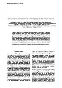
Figure 3-1: Photograph of one of the bioreactors used. Both temperature/oxygen and pH probes are behind the motor and therefore not shown. (1) DC motor connected to the bioreactor agitator. (2) (Filtered) gas entrance to the bioreactor. (3) Condenser. (4) Off gas exit (to CO2 and O2 analyzer). (5) Sampler (behind the condenser). (6) Bioreactor (glass flask inside the glass jacket). (7) Water entrance to the glass jacket. (8) Water exit of the glass jacket.
26
ARC
ARC
DO
pH
FC
Nitrogen Acid control Oxygen Basic control
Mixer Air
Feed
Antifoam
TRC Sampler Condenser
AT CO2-O2
Off gas
AT DO
AT pH
AR CO2-O2
TT Cool water (10°C) Bioreactor Hot water (50°C)
Figure 3-2: P&ID of the system used for all cultivations. Nomenclature used: AT → Analysis Transmitter. AR → Analysis Recorder. ARC → Analysis Recorder & Controller. TT → Temperature Transmitter. TRC → Temperature Recorder & Controller. FC → Flow Controller (Not used in anaerobic conditions). Glucose starvation was detected with a sudden decrease of the CO2 composition in the off-gas, and confirmed each time using Benedict's reagent (Benedict, 1909). For the fedbatch cases (conditions 1 and 2), the feed F(t) was designed for a predefined variable growth rate, and can be calculated from the reactor’s glucose and biomass mass balances, as detailed elsewhere (Villadsen & Patil, 2007): 𝛍
(𝐭)
𝐭
𝐆𝐗
𝐢
𝐅(𝐭) = 𝐆𝐬𝐞𝐭 ∙ 𝐕𝐢 𝐗 𝐢 ∙ 𝐞𝐱𝐩 {∫𝐭 𝛍𝐬𝐞𝐭 (𝐭)𝐝𝐭} 𝐅 ∙𝐘
(Equation 14)
27
With GF the glucose feed concentration [g/L], YGX the experimental glucose-biomass yield (fixed for Equation 13 in 0.469 [gDW/g] (Møller, Sharif & Olsson, 2004)), t i the time at which the feed started for a given cultivation [h], Vi and Xi the volume [L] and biomass [g/L] values at t i , respectively, and μset (t) the variable growth rate. The latter was defined as the following: 𝛍𝐬𝐞𝐭 (𝐭) = 𝐀 + 𝐁 ∙ 𝐞−𝐂𝐭
(Equation 15)
Where A and B are both 0.07 [1/h] for all aerobic cultivations, and C is 0.14 [1/h] for condition 1, and 0.07 [1/h] for condition 2. Therefore, μset (t) decays more quickly in
0.14
0.004
0.13
0.0035
0.12
0.003
0.11
0.0025
0.1
0.002
µ(set), C = 0.14 [1/h]
0.09
F [L/h]
µ(set) [1/h]
condition 1, which translates into a slower feed rate (Figure 3-3).
0.0015
µ(set), C = 0.07 [1/h] F, C = 0.14 [1/h]
0.08
0.001
F, C = 0.07 [1/h] 0.07
0.0005 0
2
4
6
8
10
t [h]
Figure 3-3: The temporal evolutions of the design growth rate (µset) and a given feed rate (F) for experimental conditions 1 (C = 0.14 [1/h]) and 2 (C = 0.07 [1/h]) are displayed, with t = 0 as the feed starting point. Condition 1 has a quicker decay in µset than condition 2, and therefore has a slower F than condition 2. For F visualization, typical experimental conditions were selected: Vi = 0.4 [L] and Xi = 4 [g/L] (for further details refer to Equation 14).
28
3.3
Assay Methods
Samples of ~5 [mL] were taken periodically from all cultivations. Biomass was measured in OD using a UV-160 UV-visible recording spectrophotometer (Shimadzu, Japan), and results were transformed to g/L using a calibration curve of 0.3797 [gDW/L/OD] for the N30 strain and of 0.3840 [gDW/L/OD] for the EC1118 strain (both determined with an infrared dryer-equipped balance (Precisa, Switzerland)).
A 2 [mL] aliquot of each sample was centrifuged for 5 minutes at 14,000 RPM and 4°C, using a Mikro 22R centrifuge (Hettich, Germany). All supernatants were kept at -80°C until the fermentation was over. Extracellular metabolites were afterwards measured by high-performance liquid chromatography (HPLC) in duplicate. 100 [µL] of a solution 27.5 [mM] H2SO4 and with 16.7 [g/L] of pivalic acid (used as internal standard) were added to 1 [mL] of each sample and each of the HPLC standards (with known concentrations of trehalose, glucose, fructose, glycerol, ethanol, citrate, malate, succinate, lactate and acetate). Afterwards, 20 [µL] of the resulting solutions were injected into a LaChrom L-7000 HPLC system (Hitachi, Japan), with an Aminex HPX87H anion-exchange column (Bio-Rad, USA) for organic acids, alcohols and sugars separation, working at 55°C with a 0.5 [mL/min] flow of mobile phase 2.5 [mM] H 2SO4 (the same concentration as the one in each sample after adding the internal standard solution). A LaChrom L-7450A diode array detector (Hitachi, Japan) was used at 210 [nm] for detecting organic acids, and a LaChrom L-7490 refraction index detector (Hitachi, Japan) for sugars and alcohols. Finally, each metabolite was quantified normalizing each area in the chromatogram by the corresponding internal standard area and using a calibration curve with the HPLC standards.
29
3.4
Reparameterization Analysis
3.4.1 General Methodology of Procedure As mentioned in the introduction, we used a novel methodology to obtain a set of identifiable and significant parameters in our dFBA model for each of the 16 experimental cultivations. As shown in Figure 3-4, the methodology starts by calculating sensitivity and identifiability for the estimated parameters of the calibration. Then, the parameters are iteratively fixed: At the end of each iteration, and depending on the regression diagnostics result, a parameter is eliminated (thus its value becomes fixed) for the next iteration. The following rules were considered for deciding which parameters to fix (for further details of each analysis see the Pre/Post Regression Diagnostics section):
1. Identifiability: when 2 parameters had a Pearson correlation coefficient larger than 0.95, different combinations of the corresponding estimated values resulted in the same objective function in the parameter estimation procedure and, consequently, the decision was to fix at least one of them. 2. Sensitivity: when the relative sensitivity of a parameter was below 0.01 for all variables, the parameter was considered to have no influence in the model, and therefore was decided to be fixed.
For most of the iterations, more than one of the above problems will arise, and therefore exploratory branches for each of the corresponding parameters are necessary, which generates a growing exploratory tree. However, because the procedure could generate an excessive number of branches, model-specific policies should be defined in order to overcome this issue. Our aim here was to find an adequate set of parameters for our model with reasonable computational times. In this work, the main strategy to reduce the exploratory tree size was to count the number of problems (identifiability and sensitivity) for each parameter at each round of the procedure. If any parameter had both problems, exploratory branches were created only for the parameters with the 2
30
problems. On the other hand, if there were only parameters with 1 of the 2 problems, we created branches for all the problematic parameters. Finally, if no parameter had any of the mentioned problems, the solution was saved for posterior analyses, and the branch no longer explored.
Figure 3-4: Methodology used in this study for obtaining dFBA models with sensitive, uncorrelated and significant parameters. As an example, a solution with 5 parameters is analyzed.
31
Once the exploratory tree concluded, the combinations that showed no identifiability or sensitivity problems were collected, and confidence coefficients (CCs) were calculated for each non-fixed parameter (Figure 3-4). The CCs had to be calculated for each of the combinations, given that their values are dependent on the combination of estimated parameters, in contrast with the sensitivity and correlation values, which remain constant regardless of the combination of estimated parameters (and therefore could be calculated only at the beginning of the procedure). If any non-fixed parameter from a solution had a CC larger than 2, it was considered that the parameter had a value not significantly different from zero, and therefore the corresponding solution was disregarded.
Finally, for each of the 16 experimental conditions, the solution with the smallest mean CC was chosen as the optimal reparameterization (Figure 3-4). This solution had a fixed parameter set (i.e. parameters eliminated by the procedure) and a non-fixed parameter set (i.e. parameters used for model calibration). To further improve the results, each of these 16 solutions were used to repeat the parameter estimation, but only with the corresponding non-fixed parameter set; the fixed parameter set had the same values than the originally estimated ones.
3.4.2 Pre/Post Regression Diagnostics In the following, we will briefly explain the regression diagnostics used in this study, as it has been thoroughly presented elsewhere (Jaqaman & Danuser, 2006; Sacher et al., 2011). Sensitivity analysis accounts for the relative impact that each parameter has in each of the model’s state variables. In our approach, we computed the relative sensitivity (Gik ), as indicated: 𝛉
𝐝𝐗 𝐢 (𝐭)
𝐢
𝐝𝛉𝐤
𝐤 𝐆𝐢𝐤 (𝐭, 𝛉𝐤 ) = 𝐗 (𝐭)
(Equation 16)
Where t is time, θk is the k-th parameter and Xi (t) is the i-th variable at time t. With all Gik values, for each time we formed a sensitivity matrix G(t), in which the k-th column
32
denotes the sensitivity of the k-th parameter on the state variables. In order to obtain a single normalized score (spanning all experimental times) of each parameter over each variable, we calculated average sensitivity as detailed in (Hao, Zak, Sauter, Schwaber & Ogunnaike, 2006). Therefore, if this score is under 0.01 in each variable for a given parameter, we chose to fix the corresponding parameter.
For identifiability calculations, the MATLAB function corrcoef was used to calculate the correlation coefficients between each column of the sensitivity matrices, and stored the information in a correlation coefficients matrix (C). If any of the matrix absolute values (besides the diagonal) is over a certain threshold (in our case |Cij| ≥ 0.95), both of the associated parameters are strongly correlated, and therefore one of both should be fixed.
For significance calculations, and also using the sensitivity matrices, we first calculated the Fisher Information Matrix (FIM) (Petersen, Gernaey & Vanrolleghem, 2001): 𝐅𝐈𝐌 = ∑𝐧𝐣=𝟏 𝐆𝐣𝐓 𝐐𝐣 𝐆𝐣
(Equation 17)
Here, Gj is the sensitivity matrix for measurement j, n is the number of measurements, and Qj is the inverse of the measurement error covariance matrix assuming white and uncorrelated noise, which is used as a weighting matrix. Using this matrix, the variances for each estimated parameter (σ2k ) were calculated as (Landaw & DiStefano III, 1984; Petersen et al., 2001): −𝟏 𝛔𝟐𝐤 = 𝐅𝐈𝐌𝐤𝐤
(Equation 18)
With the variances we computed the confidence interval (CI) with 5% significance for the k-parameter as follows: ̂𝐤 ± 𝟏. 𝟗𝟔 𝛔𝐤 ] 𝐂𝐈𝐤 = [𝛉
(Equation 19)
Where θ̂k is the estimated value of the respective parameter. Finally, coefficients of confidence (CC) were calculated as follows:
33
𝐂𝐂𝐤 =
∆(𝐂𝐈𝐤 ) ̂𝐤 𝛉
(Equation 20)
With ∆(CIk ), the CI’s length. With this metric, we determine that a parameter is not significantly different from zero if the CI contained the zero, therefore if the corresponding CC was larger than 2.
The duration to compute the whole aforementioned pre/post regression diagnostics lasted between 10 and 50 [min], depending on the experimental conditions and the computer employed (Table 2-1).
3.4.3 Cross-Calibration Once the reparameterization was performed for each of the 16 cultivations, the consistency of each solution was studied by performing a cross-calibration between the cultivations. Both the fixed and non-fixed parameter sets obtained from each fermentation were used to calibrate the remaining 7 fermentations (aerobic or anaerobic), i.e. fixing the corresponding parameters with the fixed parameter set values and fitting the data with the non-fixed parameter set. Afterwards, a cross calibration coefficient (CCC) was computed as: 𝐅
𝐂𝐂𝐂𝐢𝐣𝐤 = 𝐅𝐢𝐣𝐤 𝐣𝐣𝐤
;
𝐢, 𝐣 = 𝟏 … 𝟖 ; 𝐢 ≠ 𝐣 ;
𝐤 = {𝟎, 𝟏} (Equation 21)
Where Fijk is the objective function obtained with the i-th solution using the experimental data of the j-th cultivation, and k is an index for distinguishing between aerobiosis (k = 1) and anaerobiosis (k = 0). Therefore, if the CCCijk is close to 1, the ith solution used to calibrate the j-th experimental data is appropriate. On the other hand, if CCCijk is much larger than 1, a good fit was not possible and therefore the i-th solution is not useful for predicting different experimental conditions.
34
4
RESULTS AND ANALYSIS 4.1
Pre/post Regression Results
4.1.1 Identifiability Analysis After performing the first calibration (with all parameters) of the 16 cultivations, we encountered numerous sensitivity, identifiability and significance problems (Table 4-1). In the aerobic cultivations, the most correlated parameters were present in 3 groups (Table 4-1A). First, the glucose consumption parameters (vGmax , K G and K E ) were almost always structurally unidentifiable. This suggests that merely one parameter should be used for calibration, contrary to what is traditionally done. The second group included all 4 parameters directly related to the biomass formation in the batch stage: α, a, c and l. Here, the correlations were high in almost all fermentations, suggesting that the “suboptimal growth” effect can be achieved with just one of these parameters. Interestingly, the ethanol production yield (fE ) in the batch stage showed significant correlations with this group, indicating that in Yeast 5, under aerobic conditions, ethanol is more correlated to biomass formation than any other secondary metabolite. Furthermore, α was most of the times correlated with K E , indicating a possible connection between suboptimal growth rate and ethanol inhibition. The final group that was strongly inter-correlated belongs to the fed-batch stage, αF , vE and vGL . The relationship between biomass and ethanol also holds and an additional relation with glycerol arises, probably due to the consumption of the latter in this stage.
In anaerobic cultivations, large correlations were observed between all members of a large parameter group, that included vGmax , K G , K E , α, a, c, l, mATP and fGL (Table 4-1B). This indicates a stronger interdependence in anaerobic cultures between glucoseassociated and biomass-associated parameters, which was not observed for aerobic conditions. This is probably due to the fact that in anaerobiosis, Yeast 5 has fewer choices to produce the energetic requirements (given that the electron transport system is
35
inactive) for growth, and therefore employs less metabolic pathways, increasing the correlation between glucose consumption and biomass production. Remarkably, the glycerol production yield (and not the ethanol production yield, as in aerobic cultures) is now strongly correlated to the biomass parameters, suggesting that under anaerobic conditions, glycerol is more correlated that any other secondary metabolite to the biomass formation. Table 4-1: Percentage of times that each parametric problem arose in (A) aerobic and (B) anaerobic calibrations. Identifiability was calculated as correlations between each pair of parameters, relative sensitivity was averaged among all variables, and significance was calculated using coefficients of confidence.
(A) vGmax
|Correlation| >= 0.95 vGmax -
KG
KE
α
a
88%
KE
100% 88%
-
Α A C L
63% 38% 25% -
25% 25% 13% 13%
fL
αF
vE
vGL
vC
Average |CC| >= 2 vL sensibility = 0
13% 13%
-
13%
-
-
-
-
-
-
25%
-
13% 13%
-
13%
-
-
-
-
-
-
88%
-
13% 13% 13% 13%
-
-
-
-
-
-
75%
-
-
75% 50% 50% 38%
25% 25% 25% 25%
13% 13% 13% 13%
13% 13% 13% 13%
-
-
-
-
-
-
63% 88% 88% 100%
L
mATP
t1
t2
25%
-
13%
-
-
13%
13% 13%
-
25%
25% 13%
-
75% 88% 88% 75% 13% 25% 88% 100% 100% 13% 25% 88% 100% 88% 13% 25% 75% 100% 88% 25%
88% 100% 63% 38%
KG
fC
c
88% 25% 25% -
75% 25%
mATP 13% 13% 13% 13% 13%
fE
fGL
13%
25%
-
-
-
13%
-
-
13%
-
-
-
-
-
75%
100%
t1
-
-
-
-
-
-
-
-
-
-
-
-
-
-
-
-
-
-
-
100%
100%
t2
-
-
-
-
-
-
-
-
-
-
-
-
-
-
-
-
-
-
-
88%
100%
-
-
-
-
-
-
25%
-
-
-
-
-
-
25%
-
-
-
-
-
-
-
-
-
-
-
-
-
-
-
100%
fE
13% 13% 13% 75% 50%
50%
38% 13%
-
-
-
fGL
13% 13% 13% 25% 25%
25%
25%
-
-
-
25%
13% 13% 13%
13%
13%
-
-
-
13% 13%
-
-
-
13% 13% 13% 13% 13%
13%
13% 13%
13% 13%
fC fL
-
-
25% 13% 13% -
13% 13%
-
-
-
-
-
αF
-
-
-
-
-
-
-
-
-
-
-
-
-
-
-
vE
-
-
-
-
-
-
-
-
-
-
-
-
-
-
100%
-
75%
-
-
88%
100%
vGL
-
-
-
-
-
-
-
-
-
-
-
-
-
-
75%
75%
-
-
-
100%
100%
vC
-
-
-
-
-
-
-
-
-
-
-
-
-
-
-
-
-
-
-
-
25%
vL
-
-
-
-
-
-
-
-
-
-
-
-
-
-
-
-
-
-
-
-
25%
100% 75%
36
(B) vGmax
|Correlation| >= 0.95 vGmax -
KG
α
mATP
t1
88% 100% 75% 88% 100% 88% 63%
-
KG
88%
KE
100% 88%
-
Α A C L
75% 88% 100% 88%
63% 75% 88% 63%
KE
A
88% 63% 75%
c
t2
fE
fGL
13% 13% 75%
fL
-
13%
63% 50%
-
75% 63% 75% 75% 63% 88% 63% 100% 100% 63% 100% 75% 100% 88% 63% 88% 75% 100% 88% 63%
-
-
13% 13% 13% 13%
13% 63% 38% 13%
mATP 63% 50% 63% 63% 63% t1
-
-
-
-
-
-
13%
-
-
-
fC
75% 88% 100% 88% 63%
-
88%
l
13% 63% 13% 13%
13% 13% 75% 25% 25%
63%
63%
-
-
-
-
-
-
-
-
-
-
-
25% 63% 25% 38%
38%
100%
-
63%
100%
100% 100% 100% 100%
75%
100%
-
100%
100%
-
-
-
100%
100%
13%
13%
38%
88%
13%
-
-
-
-
-
13%
-
-
-
13% 13% 13% 13% 13%
13%
13% 13%
-
-
-
fGL
75% 63% 75% 88% 63%
75%
75% 63%
-
-
13%
13% 25% 25% 63%
25%
38% 38%
-
-
13% 25%
13% 13% 25% 25% 25%
25%
13% 13%
-
-
13% 13% 13%
-
25%
-
t2
fL
25% 25% 25% 13%
-
-
fE fC
-
88% 63% 75% 75%
Average |CC| >= 2 sensitivity = 0
13% 13% 13% -
25% 13% -
4.1.2 Sensitivity Analysis Regarding the average sensitivity, in aerobic cultivations the 5 parameters that did not had an impact in any of the model’s state variables for almost all experiments were mATP , t1 , t 2 , vE and vGL (Table 4-1A); whereas in anaerobic cultivations, the insensitive parameters were l, mATP , t1 and t 2 (Table 4-1B). The ATP maintenance and both expression thresholds (mATP , t1 and t 2 ) showed to be insensitive to all state variables in most of the fermentations, regardless of the oxygen conditions, thus not being useful for calibration of S. cerevisiae dFBA models. vE and vGL showed also to be insensitive, and because they were both correlated with αF , the latter one should be preferred for calibration. Finally, l appears as a non-sensitive parameter only in anaerobic fermentations, possibly as a consequence that, under these conditions, ergosterol and fatty acids are supplied to the medium; and therefore there is sufficient lipid availability regardless of the requirements for biomass formation.
37
4.1.3 Significance Analysis Finally, results for significance indicate that most of the parameters have CCs larger than 2, i.e. they are not significantly different from zero, in the majority of the calibrations. The more significantly estimated parameters were vGmax , fE , fGL , fC , fL , vC and vL for the aerobic cultures (Table 4-1A); and vGmax , fE , fC and fL for the anaerobic cultures (Table 4-1B). However, as mentioned before, significance tests depend on the number of estimated parameters, in contrast to sensitivity and identifiability analyses. Therefore, several significance problems were expected at this level. After fixing a group of the parameters, using other criteria such as sensitivity or identifiability (as performed in the next section), the CCs of the remaining parameters should decrease, obtaining models with significant and sensitive parameters, as well as without correlations between them.
4.2
Reparameterization Results
4.2.1 Parameter Solutions The iterative procedure described in Materials and Methods was applied to each of the 16 experimental cultivations. Thanks to the heuristic criteria described above, we obtained non-problematic solutions after an average of 6,232 iterations for aerobic and 1,858 iterations for anaerobic cultivations, which are respectively 1.2% and 11.3% of the total amount of possible combinations (Figure 4-1 and Figure 4-2). For each group of non-problematic solutions, we chose the one with the lowest average CC; and then, for each selected solution, we repeated the parameter estimation. Table A-3 shows all the non-problematic solutions obtained, and Table 4-2 indicates the best choices for each of the 16 analysis after the second calibration.
38
1.E+05
All possible combinations Combinations explored by procedure Non problematic solutions
Number of combinations
1.E+04
1.E+03
1.E+02
1.E+01
1.E+00
1.E-01 0
1
2
3
4
5
6
7
8
9
10
11
12
13
14
15
16
17
18
Number of Fixed Parameters
Figure 4-1: The average number of iterations performed by the procedure for aerobic cultivations is displayed in a logarithmic scale, along with all possible combinations and the non-problematic solutions achieved. The total number of combinations was 𝟏𝟗 ), where 19 is the total number of parameters and i is the 𝐢
calculated in each case as (
corresponding number of fixed parameters. Overall, the production and consumption parameters are most of the times non-fixed, for both aerobic and anaerobic cultivations. In the aerobic case, the most repeated non-fixed parameters were fC , fL , vC (present in 7/8 of the aerobic datasets), vL (6/8), fGL (4/8) and vGmax , α, fE and αF (3/8) (Table 4-2A). In the anaerobic case, the most repeated nonfixed parameters were vGmax (present in all anaerobic datasets), fE , fL (6/8), fC (3/8) and α (2/8) (Table 4-2B). In contrast, both gene expression thresholds (t1 and t 2 ) and two of
19
39
the biomass requirements (a and l) were not chosen as fitting parameters in any of the aerobic or anaerobic calibrations. ATP maintenance (mATP ) and the carbohydrate requirement (c) were not chosen as well as non-fixed parameters in any anaerobic condition, and only chosen once in the aerobic cultivations.
1.E+04
All possible combinations Combinations explored by procedure Non problematic solutions
Number of combinations
1.E+03
1.E+02
1.E+01
1.E+00
1.E-01 0
1
2
3
4
5
6
7
8
9
10
11
12
13
Number of Fixed Parameters
Figure 4-2: The average number of iterations performed by the procedure for anaerobic cultivations is displayed in a logarithmic scale, along with all possible combinations and the non-problematic solutions achieved. The total number of combinations was 𝟏𝟒 ), where 14 is the total number of parameters and i is the 𝐢
calculated in each case as (
corresponding number of fixed parameters. These results, together with the analyses already presented of the initial calibrations (see Pre/post Regression Results) indicate that in order to adequately calibrate a dFBA model, information such as ATP maintenance, biomass composition, and transcriptomic data is redundant if the kinetic productions and consumptions are already considered in
14
40
the parameter estimation. This is consistent with previous observations on the sensitivity of the biomass components (Varma & Palsson, 1993) and gene expression data (Hjersted & Henson, 2009). However, we expanded here those results by considering also significance and identifiability criteria, so the assessment is made now from a broader point of view. Table 4-2: The fixed and estimated parameters are presented along with their CC (only for the estimated parameters), after applying the pre/post regression procedure in the (A) aerobic cultivations and (B) anaerobic cultivations. N30
EC1118
Slow Feed
(A)
1 k
Fast Feed 2
CC
k
𝐯𝐆𝐦𝐚𝐱 1.35E+01 0.208 2.20E+01
Slow Feed
3
4
5 k
Fast Feed 6
CC
k
7
CC
k
CC
k
CC
CC
k
-
1.59E+01
-
9.95E+00
-
1.47E+01 0.078 2.45E+01 0.043 1.58E+01
-
1.98E-01
-
8 CC
k
CC
-
2.25E+01
-
𝐊𝐆
5.30E+00
-
1.38E+00 0.007 2.67E+00
3.05E+00
-
3.66E+00
-
6.86E-01 0.056 8.81E-01
-
𝐊𝐄
2.23E+01
-
1.99E+01
-
1.42E+01 0.265 2.96E+01 0.002 1.58E+01
-
3.60E+00
-
2.53E+01
-
𝛂
8.75E-01
-
7.14E-01
-
1.98E-01
-
4.05E-01
-
8.71E-01 0.063 1.97E-01
-
6.00E-01 0.067 8.95E-01 0.501
𝐚
5.81E-01
-
6.20E-01
-
6.12E-01
-
2.12E+00
-
5.06E-01
9.34E-01
-
6.19E-01
-
1.55E+00
-
𝐜
8.19E-01
-
5.47E-01
-
1.12E+00
-
5.05E-01
-
1.65E+00 0.064 1.06E+00
-
5.82E-01
-
2.23E+00
-
𝐥
1.89E+00
-
1.60E+00
-
1.63E+00
-
2.11E+00
-
2.11E+00
-
1.33E+00
-
2.47E+00
-
2.82E+00
-
𝐦𝐀𝐓𝐏 9.39E-05
-
1.85E-06
-
6.17E-03
-
1.92E-06
-
2.93E-02
-
1.20E+00 0.071 1.99E-06
-
1.99E-06
-
-
-
6.74E+00
𝐭𝟏
3.12E+00
-
4.33E+00
-
8.88E-01
-
1.75E-01
-
4.26E+00
-
6.84E-01
-
5.53E+00
-
4.03E+00
-
𝐭𝟐
8.49E+01
-
7.50E+01
-
8.42E+01
-
8.74E+01
-
7.97E+01
-
9.13E+01
-
9.80E+01
-
7.57E+01
-
𝐟𝐄
1.22E+00 0.036 1.59E+00
-
2.89E-02
-
1.93E-02
-
1.43E+00
-
9.32E-03 0.091 1.49E+00
-
1.21E+00 0.326
𝐟𝐆𝐋
1.61E-01 0.123 9.87E-02
-
5.57E-02
-
1.03E-08
-
2.23E-02 0.765 9.56E-07
𝐟𝐂
4.74E-02 0.170 4.52E-02
-
3.68E-02 0.462 4.13E-02 0.006 8.18E-03 0.418 6.95E-03 0.036 5.16E-03 0.180 6.10E-03 0.322
𝐟𝐋
7.91E-02 0.133 8.44E-02
-
1.04E-01 0.007 8.09E-02 0.007 1.77E-02 0.073 2.41E-02 0.400 1.60E-02 0.063 2.05E-02 0.146
𝛂𝐅
1.02E-01
-
1.14E-01 0.047 1.18E-01
-
𝐯𝐄
-2.78E+00
-
-9.88E+00
-
-5.03E+00
-
-4.38E+00
-
-8.40E+00
-
3.38E-02 0.164 7.34E-03 1.107
4.34E-01
-
8.89E-01
-
5.14E-01 0.258 5.33E-01
-
3.41E-01 1.496
-
1.17E-01
-
-3.96E+00
-
-9.42E+00
-
-7.67E+00
-
-3.53E+00
-
𝐯𝐆𝐋
-6.13E+00
-
-1.26E+00
-
-3.56E+00
-
-7.89E+00
-
-6.93E+00
-
-3.65E-01
-
𝐯𝐂
2.73E-01 0.706 1.47E-01 0.040 2.26E-01 0.734 1.58E-01 0.310 3.75E-02 0.646 1.34E-01 0.224 7.91E-02 0.181 5.72E-02
-
𝐯𝐋
1.82E-01 0.863 3.01E-01 0.730 6.88E-02
-
-
1.42E-01 0.401 2.47E-01 0.251 4.78E-01 0.231 2.07E-01 0.185 2.81E-01
41
N30
EC1118
Low G0
(B)
Large G0
1
2
K
CC
k
3 CC
k
Low G0 4
CC
k
Large G0
5 CC
k
6 CC
k
7 CC
k
8 CC
k
CC
𝐯𝐆𝐦𝐚𝐱 2.74E+01 0.043 1.95E+01 0.004 2.58E+01 0.020 2.86E+01 0.016 2.94E+01 0.018 1.67E+01 0.028 2.17E+01 0.019 2.06E+01 0.010 𝐊𝐆
1.57E+00
-
1.12E-02
-
5.35E-02
-
4.38E+00
-
6.86E-02
-
3.01E-01
-
5.67E+00
-
6.44E+00
-
𝐊𝐄
1.20E+01
-
2.47E+01
-
2.01E+01
-
1.55E+01
-
9.03E+00
-
2.79E+01
-
3.27E+01
-
3.13E+01
-
𝛂
9.04E-01
-
7.91E-01
-
6.32E-01
-
6.23E-01
-
8.36E-01
-
9.69E-01 0.009 8.74E-01
-
9.32E-01 0.014
𝐚
8.90E-01
-
1.22E+00
-
7.82E-01
-
8.63E-01
-
7.51E-01
-
1.54E+00
-
8.00E-01
-
1.61E+00
-
𝐜
9.21E-01
-
1.58E+00
-
1.11E+00
-
6.95E-01
-
6.59E-01
-
7.08E-01
-
7.05E-01
-
6.06E-01
-
𝐥
2.77E+00
-
3.00E+00
-
2.40E+00
-
2.28E+00
-
2.76E+00
-
1.24E+00
-
1.94E+00
-
2.29E+00
-
𝐦𝐀𝐓𝐏 9.64E-02
-
1.45E-06
-
4.07E-07
-
9.44E-02
-
1.74E-06
-
4.04E-07
-
3.60E-05
-
6.76E-07
-
𝐭𝟏
5.89E-01
-
5.28E+00
-
4.55E+00
-
4.21E+00
-
1.82E+00
-
7.09E-03
-
4.76E+00
-
4.37E+00
-
𝐭𝟐
9.81E+01
-
8.30E+01
-
9.77E+01
-
8.93E+01
-
8.49E+01
-
9.96E+01
-
9.48E+01
-
9.81E+01
-
𝐟𝐄
1.48E+00 0.068 1.36E+00 0.017 1.32E+00 0.106 1.44E+00
-
1.39E+00 0.013 3.81E-01
-
1.34E+00 0.059 1.41E+00 0.001
𝐟𝐆𝐋
4.44E-03
-
1.10E-07
-
2.74E-02
-
2.24E-01
-
1.85E-01
-
4.35E-02
-
7.04E-08
𝐟𝐂
1.51E-02
-
4.65E-02
-
1.98E-02
-
3.79E-02
-
3.89E-02 0.114 3.06E-02 0.076 3.48E-02
-
3.27E-02 0.009
𝐟𝐋
1.08E-01 0.165 1.08E-01
-
6.87E-02 0.098 7.28E-02
-
2.42E-02 0.142 2.11E-02 0.094 1.95E-02 0.043 2.14E-02 0.001
-
1.07E-01
4.2.2 Fittings Table 4-3 displays the objective function values obtained before and after each reparameterization analysis, showing in most cases a small improvement in the calibration, which is expected because it is the same parameter estimation but with fewer parameters to estimate, and with the non-estimated parameters fixed at the values obtained with the first optimization. Because the global optimum of the problem is not guaranteed when using metaheuristic optimization, calibrations with a smaller number of parameters contribute to explore the search space in more detail, thus obtaining better results. Hence, the procedure presented in this work did not only obtain models with no sensitivity, identifiability or significance problems, but also slightly improved the fitting to the experimental information.
-
42
Table 4-3: The objective function value is presented for all 16 cultivations, after the initial calibration (Initial F) and after applying the iterative procedure (Final F).
Slow feed N30 Fast feed
Aerobic Cultivations
Slow feed EC1118 Fast feed Small G0 N30 Large G0 Anaerobic Cultivations Small G0 EC1118 Large G0
Initial F
Final F
2.30E-03
2.30E-03
2.88E-03 5.81E-03 1.63E-03
2.71E-03 5.66E-03 1.55E-03
4.07E-03
3.63E-03
9.40E-03 2.23E-03 3.66E-03
8.14E-03 1.93E-03 2.82E-03
1.50E-03
1.50E-03
4.96E-04
4.83E-04
1.86E-03
1.27E-03
1.59E-03
1.59E-03
2.41E-03
2.19E-03
2.48E-03
2.35E-03
1.31E-03
1.31E-03
1.18E-03
1.18E-03
The calibrations attained after applying this procedure, together with all the experimental measurements of biomass and extracellular metabolites are displayed in Figure 4-3 (aerobic cultivations) and Figure 4-4 (anaerobic cultivations). The main metabolites detected by HPLC were glucose, citrate, lactate, glycerol and ethanol. Acetate, malate, succinate, fructose and trehalose were occasionally detected, but in lower concentrations and with significant noise, and were therefore disregarded and not included in the analysis.
43
44
Figure 4-3: (previous page) Calibrations obtained with the dFBA model after applying the pre/post regression analysis to the aerobic cultivations. Each graphic displays the experimental measures for biomass (♦), glucose (■), ethanol (▲), glycerol (×), citric (+) and lactic acid (●), together with the corresponding model prediction (continuous lines), for different experimental conditions: (A-B) N30 strain, slow feed. (C-D) N30 strain, fast feed. (E-F) EC1118 strain, slow feed. (G-H) EC1118 strain, fast feed. Overall, for the aerobic cultivations the procedure successfully calibrated citrate, lactate and ethanol, underpredicted biomass (mostly in the fed-batch stage) 5 of 8 times, slightly overpredicted glucose 2 of 8 times, and incorrectly predicted glycerol 3 of 8 times. On the other hand, the procedure successfully calibrated anaerobic cultivations for all variables with the exception of ethanol that was sometimes slightly underpredicted at the end of the batch. Clearly, the main issue in calibration was the fed-batch phase for aerobic cultivations; additional kinetics or parameters should perhaps be considered in the future when calibrating fed-batch cultures with dFBA. Nevertheless, considering that, to the best of our knowledge, this is the first time that S. cerevisiae fed-batch cultures were calibrated using dFBA, we considered the fitting procedure successful. As final considerations, we confirmed that not only all parameters are now significant (Table 4-2), but also uncorrelated (Table A-4) and have an impact in at least one variable of the model (Figure B-1 and Figure B-2). We therefore can ascertain that the models developed here have an adequate number of parameters, in the sense that with the corresponding parameters, a good fitting is obtained and, at the same time, the typical problems of too many model parameters do not arise. However, nothing can be said yet about the predictability of the models, because they have not been tested under different experimental conditions. Given that we want to find robust models, in the following we investigate the predictive capacities of each model.
45
46
Figure 4-4: (previous page) Calibrations obtained with the dFBA model after applying the pre/post regression analysis to the anaerobic cultivations. Each graphic displays the experimental measures for biomass (♦), glucose (■), ethanol (▲), glycerol (×), citric (+) and lactic acid (●), together with the corresponding model prediction (continuous lines), for different experimental conditions: (A-B) N30 strain, small G0. (C-D) N30 strain, large G0. (E-F) EC1118 strain, small G0. (G-H) EC1118 strain, large G0.
4.3
Cross-Calibration Results
The results of the cross-calibration study are displayed in Table 4-4. For both cases (aerobic and anaerobic), at least 3 of the 8 different solutions are useful for predicting several experimental conditions, i.e. the mean CCC value was close to 1 (solutions 1, 6 and 8 in the aerobic case (Table 4-4A) and 5, 6 and 8 in the anaerobic case (Table 4-4B)). The latter suggest that similar fittings can be attained in the different experimental conditions using just one of the mentioned solutions for calibration.
Remarkably, several of the CCC values are smaller than 1 (Table 4-4), suggesting that, for those cases, a given solution used to calibrate a different experimental dataset performed even better than the original solution attained by the procedure. These results show the usefulness of our technique and of the cross-calibration approach for obtaining good calibrations, which would have not been possible if we had just calibrated the data using all the parameters.
47
Table 4-4: The results of the cross calibration are presented for (A) aerobic and (B) anaerobic cultivations. Each CCC was calculated as indicated in Equation 21. The mean CCC for each solution is also presented, and the best one for each cultivation condition (aerobic/anaerobic) is blackened. N30
(A)
EC1118
Slow feed
Fast feed
Slow feed
Fast feed
1
2
3
4
5
6
7
8
1
-
0.91
1.62
2.00
1.61
0.77
1.35
1.14
1.34
2
2.01
-
3.59
6.05
9.72
6.16
11.66
19.52
8.39
3
2.94
3.87
-
1.83
9.24
4.00
15.13
12.32
7.05
4
2.13
3.09
1.11
-
6.25
2.85
9.29
8.37
4.73
5
2.22
0.97
2.44
5.33
-
0.74
1.66
17.31
4.38
6
2.99
3.78
1.02
1.84
2.07
-
2.85
2.37
2.42
7
1.99
3.73
3.52
6.93
0.97
0.72
-
12.48
4.34
8
1.46
1.32
0.89
1.87
0.79
0.72
1.37
-
1.20
Mean
Slow feed N30 Fast feed
Slow feed EC1118 Fast feed
N30
(B)
Low G0
EC1118 Large G0
Low G0
Large G0
Mean
1
2
3
4
5
6
7
8
1
-
15.79
2.45
6.15
4.71
5.99
6.87
12.92
7.84
2
9.80
-
6.50
2.17
14.66
27.12
31.57
42.33
19.17
3
2.10
9.18
-
4.32
3.05
2.82
3.83
5.99
4.47
4
9.12
9.06
5.14
-
10.22
19.34
23.69
30.77
15.33
5
0.89
1.83
0.99
2.99
-
1.15
1.30
1.83
1.57
6
1.43
3.58
2.84
2.94
1.50
-
1.44
2.26
2.28
7
5.38
5.30
3.06
3.53
1.25
1.58
-
4.01
3.45
8
1.16
1.92
2.65
1.37
1.13
1.47
1.05
-
1.53
Low G0 N30 Large G0
Low G0 EC1118 Large G0
4.3.1 Best Solutions The best solution of the 3 abovementioned calibrations is in each case highlighted in yellow in Table 4-4, and is further analyzed in the following. For aerobic cultivations,
48
the best fit corresponds to solution 8, which has as estimated parameters α, fE , fGL , fC , fL , and αF (Table 4-2A). This indicates that only using suboptimal growth rates, and minimum secondary metabolite production yields, we can generate models that are able to fit several aerobic experimental conditions of yeast growth. The rest of the parameters not only are not sensitive in the model or are correlated to others, as previously mentioned, but also do not vary significantly between conditions. For instance, a glucose maximum uptake rate of 22.5 [mmol/gDWh], a saturation constant of 0.881 [g/L] and an ethanol inhibition constant of 6.74 [g/L] (eighth column in Table 4-2A) are appropriate to represent the glucose consumption rate for most of the conditions explored, if the estimated parameters are appropriately fitted. Similar remarks can be said about the biomass requirements, the ATP maintenance, the gene expression thresholds and the fed-batch minimum secondary metabolite production rates.
On the other hand, solution 8 of the anaerobic cultivations showed to be the best one for calibration under different conditions. This set has vGmax , α, fE , fC and fL as the only parameters to estimate in order to get good fittings (Table 4-2B). This suggests that minimum glycerol production yield is less necessary for calibration for anaerobic conditions, differing from the aerobic case, and instead a good estimation of the glucose consumption rate is of more importance. Also, in this solution the ethanol inhibition constant is considerably larger (31.3 [g/L]) that in aerobic cultivations, which proposes that yeast supports higher ethanol concentrations under anoxia.
Although the two abovementioned solutions are highlighted as the best ones for explaining different aerobic or anaerobic conditions, respectively, they should not be taken as the only alternatives for calibration of new experimental conditions. Using for calibration the maximum glucose consumption rate, the ATP maintenance and some fedbatch minimum secondary metabolite production rates (Table 4-2A), instead of the suboptimal growth rate, allowed to attain good fittings also under various aerobic conditions (Table 4-4A). Likewise, not including the suboptimal growth rate or the
49
minimum citrate production yield for estimation in anaerobic conditions (Table 4-2B) can also be useful for exploring several experimental conditions (Table 4-4B). These considerations will be highly relevant when expanding the procedure to other conditions, such as other strains or medium compositions.
4.3.2 Nutrient Limitation Importance An interesting phenomenon happened in the 4-th anaerobic condition that is worthy to mention. As the last measurement was performed before the culture’s glucose limitation (Figure 4-4D), the iterative procedure concluded that with just one fitting parameter (vGmax ), a good calibration to the experimental data was possible (Table 4-2B). However, we did not achieve good calibrations in the cross-calibration analysis, with an average CCC of 15.33 (Table 4-4B). We can therefore conclude that to achieve reliable and predictive models, it is critical to have experimental measurements beyond nutrient limitation.
4.3.3 Strain Performance As a final comment, the average results between duplicates are also presented (Table 4-5), in order to visualize more directly tendencies between strains or conditions. Overall, the N30 solutions are considerably worse for calibration of the EC1118 cultures (upper-right quadrants), than vice versa (lower-left quadrants). This situation could be explained because EC1118 is a wine strain that grows in very hostile environments (low temperatures, presence of other microorganisms, high ethanol concentrations, etc.), in comparison with N30 which has been optimized to work at typical industrial conditions (30°C, pH = 5) and separated from other microorganisms. Hence, we propose that a dFBA model that represents an optimized yeast strain will be more troublesome to use for predicting the behavior of a natural strain, than the other way around. Finally, no
50
visible tendencies were obtained analyzing the different feed strategy groups in the aerobic case, or the different medium composition groups in the anaerobic case. Table 4-5: Averaged CCCs between duplicates for (A) aerobic and (B) anaerobic cultures. (A)
N30
EC1118
Slow
Fast
Slow
Fast
Slow
1.46
3.32
4.56
8.42
Fast
3.01
1.47
5.59
11.28
Slow
2.49
2.66
1.40
6.05
Fast
3.12
3.30
0.80
6.93
N30
EC1118
(B)
N30
EC1118
Low
Large
Low
Large
Low
12.79
4.32
13.12
23.43
Large
7.37
4.73
8.85
16.07
Low
1.93
2.44
1.33
1.71
Large
3.92
2.65
1.36
2.53
N30
EC1118
4.4
Approach Limitations
There are several assumptions that were made in this study that should be considered in order to understand the limitations of the model predictions. Most of them have been already mentioned (such as FBA and dFBA assumptions); here we highlight other important approximations.
4.4.1 Parameters not Included in the Study Some parameters and variables that have also been used in dFBA modeling were disregarded from our analysis. First, all parameters associated with oxygen consumption, both oxygen transfer rate (OTR) and oxygen uptake rate (OUR) kinetics (Saa, Moenne, Pérez-Correa & Agosin, 2012), were not included in the analysis. This was because the
51
fermentations were anaerobic and aerobic glucose-limited, not oxygen-limited. Therefore, in the former case there was no oxygen to model, and in the latter case oxygen was always available at sufficient concentrations thanks to an efficient control, which made dynamic modeling unnecessary (Hanly & Henson, 2011; Hjersted & Henson, 2006). In the future, experiments with small amounts of oxygen such as microaerobic or oxygen-limited fermentations should be considered in order to include in the proposed analysis oxygen parameters, such as 𝑘𝐿 𝑎 (OTR) and Monod-type kinetics (OUR).
Secondly, as previously mentioned, the growth associated maintenance (GAM) was also not included, given its correlation with non-growth associated maintenance (NGAM). Likewise, the P/O ratio, valid only for aerobic cultures (when the electron transfer system is active), was neither considered, because it is structurally unidentifiable with the ATP maintenance (Jouhten et al., 2012). In any case, for fully aerobic conditions, the P/O ratio remains constant and has been estimated around 1 using small models based on central carbon metabolism (Saks, Ventura-Clapier, Leverve, Rossi & Rigoulet, 1998) and also using Yeast 5 (Jouhten et al., 2012). Therefore, microaerobic or oxygen-limited fermentations should be performed to study appropriately this parameter.
Proton and nitrogen balances were not included in the analysis because this work focused in carbon limitation, and their supply was sufficient to avoid limitation. Finally, the CO2 production was also disregarded from the analysis, as measures of specific productivity [mmol/gDWh] were not attainable from our experimental setup. This could be solved with an additional gas flowmeter in the off-gas (Figure 3-2).
4.4.2 Fed-batch Parameters A second consideration is related to the fed-batch stage in aerobic cultivations. Here, the specific growth rate was calibrated using a suboptimal parameter (αF ), although we
52
simultaneously defined in Equation 14 the feed rate based on a predefined growth rate (μset ) (Equation 15). Also in Equation 14, we used an experimentally observed glucose to biomass yield (YGX ), instead of using the yield calculated from the model’s exchange reactions. Although these situations appear contradictory, one should bear in mind that the deduction of Equation 14 (Villadsen & Patil, 2007) has strong assumptions, such as a constant YSX through all the fermentation, and consequently should serve as a tool only for defining the feed rate, not directly imposing restrictions to the metabolic model. In addition, the metabolic model’s growth rate and glucose consumption values cannot be used to define the feed rate, because the parameter estimation cannot be performed until the fermentation ends. Therefore, the situation is unavoidable if we are performing just a couple of experiments for each condition. An interesting approach for future experiments, considering the model’s biomass underprediction in the fed-batch stage for some cultivations, could be an iterative experiment/calibration process, in which we first perform the fermentation, then calibrate the data; then redefine the growth rate and the glucose to biomass yield for a new fermentation based on the calibration results; and finally iterate until experimental and model parameters stabilize at the same value.
4.4.3 Gene Expression Parameters Further considerations must be made regarding the gene expression rules proposed. As mentioned before, the main assumptions were that the expression was strain independent, and the rules remained constant through all fermentation. These assumptions were adopted because not enough data was collected to generate more elaborated rules. As seen in Table 4-2, the expression thresholds t1 and t 2 are almost always near 4 and 100%, respectively, which means no gene deletions occurred. In the few cases that one of the thresholds was calibrated with a lower value (3 cases in aerobic and 2 cases in anaerobic cultures), some unexpressed genes arose (Table A-5), but did
53
not impact the model because the associated enzymes were already inactive (in the aerobic case, one of the many glucose transporters, and in the anaerobic case, several mitochondrial enzymes of respiration).
Evidently, better methodologies are needed in order to obtain relevant information from gene expression in dFBA. An interesting improvement could be to measure gene expression through the studied fermentation, and integrate the results in the analysis as temporal Boolean rules using a delay parameter, as reported previously (Covert, Knight, Reed, Herrgård & Palsson, 2004; Covert, Schilling & Palsson, 2001). This delay parameter could be fixed according to literature or also estimated from experimental data. Also, additional levels of information such as proteomics, metabolomics and fluxomics would probably aid even more in the elucidation of a robust mathematical representation of the connection between gene expression and reaction fluxes in dFBA modeling. Nevertheless, we once again highlight that using only microarray information as constant on/off rules does not provide additional insights if the kinetics of the system are well characterized (Hjersted & Henson, 2009).
4.4.4 Additional Considerations Two final remarks are necessary at this point. First, it is worthy to mention that the presented analysis is based on local sensitivity, identifiability and significance tools. Alternatively, one could use global tools such as structural identifiability analysis (Balsa-Canto et al., 2010) or bifurcation theory (Kruger, Ratcliffe & Steuer, 2007), but would require extensive symbolic manipulations and more intensive computational simulations. We overcome this issue by showing through cross-calibration that we can attain models that, although locally analyzed, are predictive for different conditions. Second, it is important to notice that given the relatively extensive computational time that the parameter estimation requires (Table 2-1), the approach is restrained to a reasonable number of studied parameters; more parameters will eventually prevent the
54
optimization algorithm to find a good solution. Consequently, future efforts should concentrate in adapting the presented methodology to models with more parameters, considering that novel models that account for all known cellular process have thousands of parameters (Karr et al., 2012).
55
5
CONCLUSION
Since the first dFBA model was formulated and validated (Mahadevan et al., 2002), significant efforts of the metabolic modeling community have been conducted to further improve such models (Feng et al., 2010), in order to broaden predictions to different conditions and metabolic engineering applications, such as recombinant protein production (Meadows et al., 2010; Oddone et al., 2009), overproduction of ethanol (Hjersted et al., 2007) and bioremediation (Zhuang et al., 2011). Nonetheless, few experimental conditions were explored in most of these works, and there was a lack of certainty of which dFBA parameters were relevant and which were not.
Here, we have developed a yeast dFBA model that comprises several parameters, kinetics and dynamics traditionally included in this type of models, and novel features not accounted until now, such as a sequential optimization (biomass maximization and total flux minimization), and parameters such as condition-specific biomass requirements, minimum secondary metabolite production rates for both batch and fedbatch stages, and gene expression thresholds. Also, GSMM Yeast 5 was used here for the first time in fed-batch simulations. More importantly, the model presented is the first yeast dFBA model in literature to be experimentally validated using aerobic fed-batch cultivations. Furthermore, the analysis presented is unique, in the sense that for the first time several conditions (aerobic/anaerobic, different strains, etc.) are used for calibration of the same model, which gave numerous insights into the behavior of dFBA models and yeast metabolism.
We also showed that several sensitivity, identifiability and significance problems arise in this kind of models, which can severely hamper their utility, since the parameter estimation procedure gets computationally costly and unreliable. To solve this issue, we proposed an iterative procedure based on pre/post regression diagnostics that generates reparameterizations with problem-free parameters. Moreover, we cross-calibrated these
56
results to obtain solutions that are useful among several experimental conditions. Glucose consumption, suboptimal growth rate and secondary metabolite production yields were found to be the most important parameters in most cases. Other information, like gene expression constant Boolean rules, biomass requirements and ATP maintenance is of less relevance when calibrating these models, an observation confirmed for the first time from a global perspective. Finally, we have also pinpointed improvements in this modeling approach that could further increase performance and predictability. One of the main uses of GSMM models – using both static and dynamic approaches – is as a guide for genetic modifications, i.e. knock-outs (gene deletions), knock-ins (additions), knock-downs (sub-expressions) or knock-ups (over-expressions), in order to overproduce a metabolite of interest (Alper, Jin, Moxley & Stephanopoulos, 2005; Bro, Regenberg, Förster & Nielsen, 2006; Hjersted et al., 2007). To this end, a significant amount of computational tools are now available, which using as input a GSMM can propose one or more of the mentioned modifications (Copeland et al., 2012; Park et al., 2009). Still, in order to have confident predictions, the models employed should be appropriately calibrated, otherwise erroneous predictions could occur. Therefore, the model presented in this work is expected to have important benefits when experimenting in silico and designing metabolic engineering strategies.
57
6
ABBREVIATIONS
ATP
Adenosine triphosphate
CC
Confidence coefficient
CCC
Cross calibration coefficient
CHO
Chinese hamster ovary
CI
Confidence interval
COBRA
Constraint-based reconstruction and analysis
DO
Dissolved oxygen
dFBA
Dynamic flux balance analysis
eSS
Enhanced scatter search
FBA
Flux balance analysis
FIM
Fisher information matrix
GAM
Growth associated maintenance
gDW
Gram of dry weight cell
GSMM
Genome-scale metabolic model
HPLC
High-performance liquid chromatography
LB
Lower bound
LP
Linear programming
NGAM
Non-growth associated maintenance
OD
Optical density
ODE
Ordinary differential equation
OTR
Oxygen transfer rate
58
OUR
Oxygen uptake rate
P&ID
Process and Instrumentation Diagram
QP
Quadratic programming
SBML
Systems biology markup language
SGD
Saccharomyces Genome Database
SPELL
Serial Pattern of Expression Levels Locator
SSm
Scatter search for Matlab®
UB
Upper bound
59
7
OUTREACH
The contents of this thesis were submitted for publication to the journal “Metabolic Engineering”. This work was also partially presented in three academic meetings:
Sánchez, B.J.; Pérez-Correa, J.R.; Agosin, E. Reparametrización de un modelo dinámico del metabolismo celular de S. cerevisiae. In: LXXXII Meeting of the Chilean Mathematical Society. Olmué, Chile. 7 – 9 Nov., 2013 (oral presentation).
Sánchez, B.J.; Pérez-Correa, J.R.; Agosin, E. Reparameterization analysis of a S. cerevisiae dynamic genome-scaled metabolic model. In: III Copenhagen Bioscience Conference: Cell Factories and Biosustainability. Copenhagen, Denmark. 5 – 8 May, 2013 (poster).
Sánchez, B.J.; Pérez-Correa, J.R.; Agosin, E. Modelación metabólica dinámica a escala genómica para la producción de terpenos en S. cerevisiae. In: I Chilean Conference of Biotechnology Engineering Students. Antofagasta, Chile. 17 – 19 Oct., 2012 (poster).
60
REFERENCES Aceituno, F. F., Orellana, M., Torres, J., Mendoza, S., Slater, A. W., Melo, F., & Agosin, E. (2012). Oxygen response of the wine yeast Saccharomyces cerevisiae EC1118 grown under carbon-sufficient, nitrogen-limited enological conditions. Applied and Environmental Microbiology, 78(23), 8340–8352. Åkesson, M., Förster, J., & Nielsen, J. (2004). Integration of gene expression data into genome-scale metabolic models. Metabolic Engineering, 6(4), 285–293. Alper, H., Jin, Y.-S., Moxley, J. F., & Stephanopoulos, G. (2005). Identifying gene targets for the metabolic engineering of lycopene biosynthesis in Escherichia coli. Metabolic Engineering, 7(3), 155–164. Antoniewicz, M. R. (2013). Dynamic metabolic flux analysis-tools for probing transient states of metabolic networks. Current Opinion in Biotechnology, 24(6), 973–978. Balsa-Canto, E., Alonso, A., & Banga, J. (2010). An iterative identification procedure for dynamic modeling of biochemical networks. BMC Systems Biology, 4(11). Balsa-Canto, E., Rodriguez-Fernandez, M., & Banga, J. (2007). Optimal design of dynamic experiments for improved estimation of kinetic parameters of thermal degradation. Journal of Food Engineering, 82(2), 178–188. Becker, S. a, Feist, A. M., Mo, M. L., Hannum, G., Palsson, B. Ø., & Herrgard, M. J. (2007). Quantitative prediction of cellular metabolism with constraint-based models: the COBRA Toolbox. Nature Protocols, 2(3), 727–738. Benedict, S. R. (1909). A reagent for the detection of reducing sugars. Journal of Biological Chemistry, 5(5), 485–487. Bornstein, B. J., Keating, S. M., Jouraku, A., & Hucka, M. (2008). LibSBML: an API library for SBML. Bioinformatics, 24(6), 880–881. Bro, C., Regenberg, B., Förster, J., & Nielsen, J. (2006). In silico aided metabolic engineering of Saccharomyces cerevisiae for improved bioethanol production. Metabolic Engineering, 8(2), 102–111. Cárcamo, M., Saa, P. A., Torres, J., Torres, S., Mandujano, P., Pérez-Correa, J. R., & Agosin, E. (2013). Effective dissolved oxygen control strategy for high cell-density cultures. International Journal of Computers Communication & Control, (accepted).
61
Cherry, J. M., Hong, E. L., Amundsen, C., Balakrishnan, R., Binkley, G., Chan, E. T., … Wong, E. D. (2012). Saccharomyces Genome Database: the genomics resource of budding yeast. Nucleic Acids Research, 40(D1), D700–D705. Chu, Y., & Hahn, J. (2008). Integrating parameter selection with experimental design under uncertainty for nonlinear dynamic systems. AIChE Journal, 54(9), 2310–2320. Copeland, W. B., Bartley, B. a., Chandran, D., Galdzicki, M., Kim, K. H., Sleight, S. C., … Sauro, H. M. (2012). Computational Tools for Metabolic Engineering. Metabolic Engineering, 14(3), 270–280. Covert, M. W., Knight, E. M., Reed, J. L., Herrgård, M. J., & Palsson, B. Ø. (2004). Integrating high-throughput and computational data elucidates bacterial networks. Nature, 429(6987), 92–96. Covert, M. W., Schilling, C. H., & Palsson, B. Ø. (2001). Regulation of gene expression in flux balance models of metabolism. Journal of Theoretical Biology, 213(1), 73–88. Covert, M. W., Xiao, N., Chen, T. J., & Karr, J. R. (2008). Integrating metabolic, transcriptional regulatory and signal transduction models in Escherichia coli. Bioinformatics, 24(18), 2044–2050. Curran, K. A., Crook, N. C., & Alper, H. S. (2012). Using flux balance analysis to guide microbial metabolic engineering. Methods in Molecular Biology, 834, 197–216. Dennis, J. E., Gay, D. M., & Walsh, R. E. (1981). An adaptive nonlinear least-squares algorithm. ACM Transactions on Mathematical Software, 7(3), 348–368. Diderich, J. A., Schepper, M., Van Hoek, P., Luttik, M. A. H., Van Dijken, J. P., Pronk, J. T., … Kruckeberg, A. L. (1999). Glucose Uptake Kinetics and Transcription of HXTGenes in Chemostat Cultures of Saccharomyces cerevisiae. Journal of Biological Chemistry, 274(22), 15350–15359. Dobson, P. D., Smallbone, K., Jameson, D., Simeonidis, E., Lanthaler, K., Pir, P., … Mendes, P. (2010). Further developments towards a genome-scale metabolic model of yeast. BMC Systems Biology, 4(1). Duarte, N. C., Herrgård, M. J., & Palsson, B. Ø. (2004). Reconstruction and validation of Saccharomyces cerevisiae iND750, a fully compartmentalized genome-scale metabolic model. Genome Research, 14(7), 1298–1309.
62
Edwards, J. S., & Palsson, B. Ø. (2000). The Escherichia coli MG1655 in silico metabolic genotype: Its definition, characteristics, and capabilities. Proceedings of the National Academy of Sciences, 97(10), 5528–5533. Egea, J. A., & Balsa-Canto, E. (2009). Dynamic optimization of nonlinear processes with an enhanced scatter search method. Industrial & Engineering Chemical Research, 48(9), 4388–4401. Egea, J. A., Rodriguez-Fernandez, M., Banga, J., & Martí, R. (2006). Scatter search for chemical and bio-process optimization. Journal of Global Optimization, 37(3), 481–503. Feng, X., Page, L., Rubens, J., Chircus, L., Colletti, P., Pakrasi, H. B., & Tang, Y. J. (2010). Bridging the gap between fluxomics and industrial biotechnology. Journal of Biomedicine & Biotechnology, 2010. Feng, X., Xu, Y., Chen, Y., & Tang, Y. J. (2012). Integrating flux balance analysis into kinetic models to decipher the dynamic metabolism of Shewanella oneidensis MR-1. PLoS Computational Biology, 8(2). Förster, J., Famili, I., Fu, P., Palsson, B. Ø., & Nielsen, J. (2003). Genome-scale reconstruction of the Saccharomyces cerevisiae metabolic network. Genome Research, 13(2), 244–253. Gao, J., Gorenflo, V. M., Scharer, J. M., & Budman, H. M. (2008). Dynamic metabolic modeling for a MAB bioprocess. Biotechnology Progress, 23(1), 168–181. Gianchandani, E. P., Chavali, A. K., & Papin, J. A. (2010). The application of flux balance analysis in systems biology. Wiley Interdisciplinary Reviews: Systems Biology and Medicine, 2(3), 372–382. Gurobi. (2013). version 5.5.0. Houston, Texas: Gurobi Optimization, Inc. Hanly, T. J., & Henson, M. A. (2011). Dynamic flux balance modeling of microbial cocultures for efficient batch fermentation of glucose and xylose mixtures. Biotechnology and Bioengineering, 108(2), 376–385. Hanly, T. J., & Henson, M. A. (2013). Dynamic metabolic modeling of a microaerobic yeast co-culture: predicting and optimizing ethanol production from glucose/xylose mixtures. Biotechnology for biofuels, 6(44). Hanly, T. J., Urello, M., & Henson, M. A. (2012). Dynamic flux balance modeling of S. cerevisiae and E. coli co-cultures for efficient consumption of glucose/xylose mixtures. Applied Microbiology and Biotechnology, 93(6), 2529–2541.
63
Hao, H., Zak, D., Sauter, T., Schwaber, J., & Ogunnaike, B. (2006). Modeling the VPAC2-activated cAMP/PKA signaling pathway: from receptor to circadian clock gene induction. Biophysical Journal, 90(5), 1560–1571. Heavner, B. D., Smallbone, K., Barker, B., Mendes, P., & Walker, L. P. (2012). Yeast 5 - an expanded reconstruction of the Saccharomyces cerevisiae metabolic network. BMC Systems Biology, 6(55). Heavner, B. D., Smallbone, K., Price, N. D., & Walker, L. P. (2013). Version 6 of the consensus yeast metabolic network refines biochemical coverage and improves model performance. Database, 2013(bat059). Henry, C. S., DeJongh, M., Best, A. a, Frybarger, P. M., Linsay, B., & Stevens, R. L. (2010). High-throughput generation, optimization and analysis of genome-scale metabolic models. Nature Biotechnology, 28(9), 977–982. Herrgård, M. J., Swainston, N., Dobson, P., Dunn, W. B., Arga, K. Y., Arvas, M., … Kell, D. B. (2008). A consensus yeast metabolic network reconstruction obtained from a community approach to systems biology. Nature Biotechnology, 26(10), 1155–1160. Hibbs, M. A., Hess, D. C., Myers, C. L., Huttenhower, C., Li, K., & Troyanskaya, O. G. (2007). Exploring the functional landscape of gene expression: directed search of large microarray compendia. Bioinformatics, 23(20), 2692–2699. Hjersted, J. L., & Henson, M. A. (2006). Optimization of fed-batch Saccharomyces cerevisiae fermentation using dynamic flux balance models. Biotechnology Progress, 22(5), 1239–1248. Hjersted, J. L., & Henson, M. A. (2009). Steady-state and dynamic flux balance analysis of ethanol production by Saccharomyces cerevisiae. IET Systems Biology, 3(3), 167– 179. Hjersted, J. L., Henson, M. A., & Mahadevan, R. (2007). Genome-Scale Analysis of Saccharomyces cerevisiae Metabolism and Ethanol Production in Fed-Batch Culture. Biotechnology & Bioengineering, 97(5), 1190–1204. Höffner, K., Harwood, S. M., & Barton, P. I. (2013). A reliable simulator for dynamic flux balance analysis. Biotechnology and Bioengineering, 110(3), 792–802. Holzhütter, H. (2004). The principle of flux minimization and its application to estimate stationary fluxes in metabolic networks. European Journal of Biochemistry, 271(14), 2905–2922.
64
Jacquez, J. A., & Greif, P. (1985). Numerical parameter identifiability and estimability: Integrating identifiability, estimability, and optimal sampling design. Mathematical Biosciences, 77(1-2), 201–227. Jaqaman, K., & Danuser, G. (2006). Linking data to models: data regression. Nature Reviews. Molecular Cell Biology, 7(11), 813–819. Jouhten, P., Wiebe, M., & Penttilä, M. (2012). Dynamic flux balance analysis of the metabolism of Saccharomyces cerevisiae during the shift from fully respirative or respirofermentative metabolic states to anaerobiosis. The FEBS Journal, 279(18), 3338– 3354. Karr, J. R., Sanghvi, J. C., Macklin, D. N., Gutschow, M. V, Jacobs, J. M., Bolival, B., … Covert, M. W. (2012). A whole-cell computational model predicts phenotype from genotype. Cell, 150(2), 389–401. Keating, S. M., Bornstein, B. J., Finney, A., & Hucka, M. (2006). SBMLToolbox: an SBML toolbox for MATLAB users. Bioinformatics, 22(10), 1275–1277. Kitano, H. (2002). Systems biology: a brief overview. Science, 295(5560), 1662–1664. Kruger, N., Ratcliffe, G., & Steuer, R. (2007). Computational approaches to the topology, stability and dynamics of metabolic networks. Phytochemistry, 68(16), 2139– 2151. Lai, L.-C., Kosorukoff, A. L., Burke, P. V, & Kwast, K. E. (2006). Metabolic-statedependent remodeling of the transcriptome in response to anoxia and subsequent reoxygenation in Saccharomyces cerevisiae. Eukaryotic Cell, 5(9), 1468–89. Landaw, E. M., & DiStefano III, J. J. (1984). Multiexponential, multicompartmental, and noncompartmental modeling. II. Data analysis and statistical considerations. American Journal of Physiology, 246(5), R665–R677. Mahadevan, R., Edwards, J. S., & Doyle III, F. J. (2002). Dynamic flux balance analysis of diauxic growth in Escherichia coli. Biophysical Journal, 83(3), 1331–1340. MATLAB. (2013). version 8.1 (R2013a). Natick, Massachusetts: The MathWorks Inc. Meadows, A. L., Karnik, R., Lam, H., Forestell, S., & Snedecor, B. (2010). Application of dynamic flux balance analysis to an industrial Escherichia coli fermentation. Metabolic Engineering, 12(2), 150–160.
65
Møller, K., Sharif, M. Z., & Olsson, L. (2004). Production of fungal α-amylase by Saccharomyces kluyveri in glucose-limited cultivations. Journal of Biotechnology, 111(3), 311–318. Nolan, R. P., & Lee, K. (2011). Dynamic model of CHO cell metabolism. Metabolic Engineering, 13(1), 108–124. Nookaew, I., Jewett, M. C., Meechai, A., Thammarongtham, C., Laoteng, K., Cheevadhanarak, S., … Bhumiratana, S. (2008). The genome-scale metabolic model iIN800 of Saccharomyces cerevisiae and its validation: a scaffold to query lipid metabolism. BMC Systems Biology, 2(71). Nookaew, I., Olivares-hernández, R., Bhumiratana, S., & Nielsen, J. (2011). GenomeScale Metabolic Models of Saccharomyces cerevisiae. (J. I. Castrillo & S. G. Oliver, Eds.)Methods in Molecular Biology, 759(3), 445–463. Oberhardt, M. a, Palsson, B. Ø., & Papin, J. a. (2009). Applications of genome-scale metabolic reconstructions. Molecular Systems Biology, 5(320). Oddone, G. M., Mills, D. a, & Block, D. E. (2009). A dynamic, genome-scale flux model of Lactococcus lactis to increase specific recombinant protein expression. Metabolic Engineering, 11(6), 367–381. Orellana, M., Aceituno, F. F., Slater, A. W., Almonacid, L. I., Melo, F., & Agosin, E. (2013). Metabolic and transcriptomic response of the wine yeast Saccharomyces cerevisiae strain EC1118 after an oxygen impulse under carbon sufficient, nitrogenlimited fermentative conditions. FEMS Yeast Research, (submitted). Orth, J. D., Thiele, I., & Palsson, B. Ø. (2010). What is flux balance analysis? Nature Biotechnology, 28(3), 245–248. Osterlund, T., Nookaew, I., & Nielsen, J. (2012). Fifteen years of large scale metabolic modeling of yeast: developments and impacts. Biotechnology Advances, 30(5), 979–988. Park, J. M., Kim, T. Y., & Lee, S. Y. (2009). Constraints-based genome-scale metabolic simulation for systems metabolic engineering. Biotechnology Advances, 27(6), 979–988. Petersen, B., Gernaey, K., & Vanrolleghem, P. A. (2001). Practical identifiability of model parameters by combined respirometric-titrimetric measurements. Water Science and Technology, 43(7), 347–355.
66
Pizarro, F., Varela, C., Martabit, C., Bruno, C., Pérez-Correa, J. R., & Agosin, E. (2007). Coupling kinetic expressions and metabolic networks for predicting wine fermentations. Biotechnology and Bioengineering, 98(5), 986–998. Provost, A., & Bastin, G. (2004). Dynamic metabolic modelling under the balanced growth condition. Journal of Process Control, 14(7), 717–728. Provost, A., Bastin, G., Agathos, S. N., & Schneider, Y.-J. (2006). Metabolic design of macroscopic bioreaction models: application to Chinese hamster ovary cells. Bioprocess and Biosystems Engineering, 29(5-6), 349–366. Saa, P. A., Moenne, M. I., Pérez-Correa, J. R., & Agosin, E. (2012). Modeling oxygen dissolution and biological uptake during pulse oxygen additions in oenological fermentations. Bioprocess and Biosystems Engineering, 35(7), 1167–78. Sacher, J., Saa, P., Cárcamo, M., López, J., Gelmi, C., & Pérez-Correa, J. R. (2011). Improved calibration of a solid substrate fermentation model. Electronic Journal of Biotechnology, 14(5). Sainz, J., Pizarro, F., Pérez-Correa, J. R., & Agosin, E. (2003). Modeling of yeast metabolism and process dynamics in batch fermentation. Biotechnology and Bioengineering, 81(7), 818–828. Saks, V. A., Ventura-Clapier, R., Leverve, X., Rossi, A., & Rigoulet, M. (Eds.). (1998). Bioenergetics of the Cell: Quantitative Aspects. Boston, USA: Springer. Schellenberger, J., Que, R., Fleming, R. M. T., Thiele, I., Orth, J. D., Feist, A. M., … Palsson, B. Ø. (2011). Quantitative prediction of cellular metabolism with constraintbased models: the COBRA Toolbox v2.0. Nature Protocols, 6(9), 1290–1307. Schuetz, R., Zamboni, N., Zampieri, M., Heinemann, M., & Sauer, U. (2012). Multidimensional optimality of microbial metabolism. Science, 336(6081), 601–604. Smith, W. R., & Missen, R. W. (2003). Sensitivity Analysis in Chemical Education: Part 1. Introduction and Application to Explicit Models. Chemical Engineering Education, 2003(Summer), 222–227. Sohn, S. B., Graf, A. B., Kim, T. Y., Gasser, B., Maurer, M., Ferrer, P., … Lee, S. Y. (2010). Genome-scale metabolic model of methylotrophic yeast Pichia pastoris and its use for in silico analysis of heterologous protein production. Biotechnology Journal, 5(7), 705–715.
67
Sriram, K., Rodriguez-Fernandez, M., & Doyle, F. J. (2012). Modeling cortisol dynamics in the neuro-endocrine axis distinguishes normal, depression, and posttraumatic stress disorder (PTSD) in humans. PLoS Computational Biology, 8(2). Stephanopoulos, G., Aristidou, A. A., & Nielsen, J. (1998). Metabolic Engineering: Principles and Methodologies. San Diego, USA: Academic Press. Tepeli, A., & Hortaçsu, A. (2008). A fuzzy logic approach for regulation in flux balance analysis. Biochemical Engineering Journal, 39(1), 137–148. Thiele, I., & Palsson, B. Ø. (2010). A protocol for generating a high-quality genomescale metabolic reconstruction. Nature Protocols, 5(1), 93–121. Vargas, F. a, Pizarro, F., Pérez-Correa, J. R., & Agosin, E. (2011). Expanding a dynamic flux balance model of yeast fermentation to genome-scale. BMC Systems Biology, 5(75). Varma, A., & Palsson, B. Ø. (1993). Metabolic Capabilities of Escherichia coli II. Optimal Growth Patterns. Journal of Theoretical Biology, 165(4), 503–522. Varma, A., & Palsson, B. Ø. (1994). Stoichiometric flux balance models quantitatively predict growth and metabolic by-product secretion in wild-type Escherichia coli W3110. Applied and Environmental Microbiology, 60(10), 3724–3731. Villadsen, J., & Patil, K. R. (2007). Optimal fed-batch cultivation when mass transfer becomes limiting. Biotechnology and Bioengineering, 98(3), 706–710. Yin, W. (2011). Gurobi Mex: A MATLAB interface for Gurobi. Retrieved from http://convexoptimization.com/wikimization/index.php/gurobi_mex Zhuang, K., Izallalen, M., Mouser, P., Richter, H., Risso, C., Mahadevan, R., & Lovley, D. R. (2011). Genome-scale dynamic modeling of the competition between Rhodoferax and Geobacter in anoxic subsurface environments. The ISME Journal, 5(2), 305–316. Zomorrodi, A. R., Suthers, P. F., Ranganathan, S., & Maranas, C. D. (2012). Mathematical optimization applications in metabolic networks. Metabolic Engineering, 14(6), 672–686.
68
APPENDIX
69
APPENDIX A: SUPPLEMENTARY TABLES Table A-1: Calibration comparison between Yeast 5 and Yeast 6 for two typical cultivations. The objective function value (F) and the computation time (t) are displayed.
GSMM used
Aerobic Fed-batch
Anaerobic Batch
F
t
F
t
Yeast 5 (Heavner et al., 2012)
2.4E-03
13.1 [h]
1.5E-03
7.2 [h]
Yeast 6 (Heavner et al., 2013)
5.5E-03
21.2 [h]
1.1E-02
10.6 [h]
70
Table A-2: The SGD names of the essential genes for aerobic and anaerobic growth in the genome-scale metabolic model Yeast 5 (Heavner et al., 2012) are presented. The genes that are only essential for one condition but not for the other one are highlighted. As it has been done regularly (Edwards & Palsson, 2000; Zomorrodi et al., 2012), a gene is defined essential if by deleting it (constraining in zero all associated reaction fluxes) growth is not achieved when performing FBA. Essential Genes for Aerobic Growth
Essential Genes for Anaerobic Growth
YBL033C
YEL021W
YIL094C
YMR296C
YAR015W
YDR408C
YJL088W
YNL220W
YBR029C
YER003C
YIL116W
YMR298W
YBL033C
YDR454C
YJL130C
YNL277W
YBR041W
YER023W
YIR034C
YMR300C
YBR029C
YDR487C
YJL153C
YNL316C
YBR115C
YER026C
YJL088W
YNL003C
YBR041W
YEL021W
YJR016C
YNR016C
YBR126C
YER043C
YJL130C
YNL037C
YBR115C
YER003C
YJR073C
YNR050C
YBR153W
YER052C
YJL153C
YNL220W
YBR126C
YER005W
YJR137C
YOL058W
YBR166C
YER055C
YJL167W
YNL277W
YBR153W
YER023W
YJR139C
YOL066C
YBR192W
YER069W
YJR016C
YNL280C
YBR166C
YER026C
YJR148W
YOL140W
YBR248C
YER090W
YJR073C
YNL316C
YBR192W
YER043C
YKL001C
YOL143C
YBR256C
YER091C
YJR137C
YNR016C
YBR196C
YER052C
YKL004W
YOR074C
YBR265W
YFL045C
YJR139C
YNR043W
YBR248C
YER055C
YKL024C
YOR095C
YCL009C
YFR025C
YJR148W
YNR050C
YBR256C
YER069W
YKL060C
YOR128C
YCL018W
YFR030W
YKL001C
YOL058W
YBR265W
YER090W
YKL067W
YOR130C
YCL030C
YGL001C
YKL004W
YOL066C
YCL009C
YER091C
YKL152C
YOR136W
YCR034W
YGL009C
YKL024C
YOL140W
YCL018W
YFL045C
YKL182W
YOR202W
YCR053W
YGL012W
YKL067W
YOL143C
YCL030C
YFR025C
YKL211C
YOR236W
YDL015C
YGL026C
YKL182W
YOR074C
YCR012W
YFR030W
YKL216W
YPL231W
YDL055C
YGL148W
YKL211C
YOR095C
YCR034W
YGL009C
YLR355C
YPR021C
YDL182W
YGL154C
YKL216W
YOR130C
YCR053W
YGL026C
YLR359W
YPR035W
YDR007W
YGL234W
YLR100W
YOR136W
YDL015C
YGL148W
YLR372W
YPR060C
YDR062W
YGR060W
YLR355C
YOR175C
YDL055C
YGL154C
YLR420W
YPR113W
YDR074W
YGR061C
YLR359W
YOR202W
YDL182W
YGL234W
YML008C
YPR167C
YDR127W
YGR175C
YLR372W
YOR236W
YDR007W
YGR061C
YMR062C
YPR183W
YDR158W
YGR204W
YLR420W
YPL028W
YDR062W
YGR204W
YMR108W
YDR226W
YHR007C
YML008C
YPL117C
YDR074W
YGR240C
YMR202W
YDR234W
YHR018C
YML126C
YPL231W
YDR127W
YHR018C
YMR205C
YDR353W
YHR025W
YMR062C
YPR035W
YDR158W
YHR025W
YMR217W
YDR354W
YHR042W
YMR108W
YPR060C
YDR226W
YHR208W
YMR296C
YDR367W
YHR072W
YMR202W
YPR113W
YDR234W
YIL020C
YMR298W
YDR408C
YHR190W
YMR208W
YPR167C
YDR353W
YIL094C
YMR300C
YDR454C
YHR208W
YMR217W
YPR183W
YDR354W
YIL116W
YNL003C
YDR487C
YIL020C
YMR220W
YDR367W
YIR034C
YNL037C
71
Table A-3: All solutions with no identifiability, sensitivity and significance problems are shown below, for (A) aerobic and (B) anaerobic cultivations. The fixed parameters are highlighted, and the chosen solution in each case is highlighted with a bold box. (A.1) N30 Strain – Slow Feed – 1 Fixed Parameters 1 2 3 4 5 6 7 8 9 10 11 12 13 14 15 16 17 18 19 20 21 22 23 24 25 26 27 28
2 1 1 1 1 1
2 2 2 2 2 2 2
1 1 1 1 1 1 1 1 1 1 1 1 1 1 1 1 1
2 2 2 2 2 2 2 2 2 2 2
4
5
6
8
9
10
16
17
3.50E-01
3 3
4 4 4 4 4 4 4 4 4 4 4 4 4 4 4 4
5 5 5 5
6 6 6
8 8 8 8 8 8 8 8 8 8 8 8 8 8 8 8 8 8 8 8 8 8 8 8 8 8 8
9 9 9 9 9 9 9 9 9 9 9 9 9 9 9 9 9 9 9 9 9 9 9 9 9 9 9
10 10 10 10 10 10 10 10 10 10 10 10 10 10 10 10 10 10 10 10 10 10 10 10 10 10 10
15 15 15 15 15 15 15
16 16 16 16 16 16 16 16 16 16 16 16 16 16 16 16 16 16 16 16 16 16 16 16 16 16 16
17 17 17 17 17 17 17 17 17 17 17 17 17 17 17 17 17 17 17 17 17 17 17 17 17 17 17
3.69E-01 3.31E-01 3.07E-01 3.31E-01 3.74E-01 3.01E-01 3.28E-01 3.18E-01 3.07E-01 3.34E-01 3.88E-01 3.57E-01 3.55E-01 3.36E-01 3.19E-01 3.26E-01 3.06E-01 3.07E-01 3.16E-01 3.13E-01 3.35E-01 3.07E-01 3.32E-01 3.83E-01 3.06E-01 3.35E-01 3.75E-01
7
8
9
10
15
16
17
3.01E-01
7
8 8 8 8 8 8 8 8 8
9 9 9 9 9 9 9 9 9
10 10 10 10 10 10 10 10 10
15 15 15 15 15 15 15 15 15
16 16 16 16 16 16 16 16 16
17 17 17 17 17 17 17 17 17
3.29E-01 3.19E-01 3.39E-01 3.21E-01 3.30E-01 3.06E-01 3.09E-01 3.15E-01 3.18E-01
3 3 3 3 3 3 3 3 3 3 3 3
3 3 3
4 4 4 4 4 4 4 4 4 4
3 3 3
5 5 5 5 5 5 5 5 5 5 5 5 5 5 5 5 5 5 5 5
29
2
3
4
5
30 31 32 33 34 35 36 37 38
2 2 2 2 2 2 2
3 3 3 3 3 3
4 4 4 4 4
5 5 5 5
1 1 1 1 1 1
2
mean(CC)
3
3 3
4 4 4
5 5 5 5
6 6 6 6
7 7 7 7 7 7 7
6 6 6 7 6 6 6 6 6 6 6 6 6 6
7 7 7 7 7 7 7 7 7 7
6 6 6 7 6 6 6 6 6 6
7 7 7 7 7
11 11 11 11 11 11 15 15 11 11 11 11 11 11 11
11 11 11 11
11 11 11 11 11 11 11 11 11
72
(A.2) N30 Strain – Slow Feed – 2 Fixed Parameters 1
1
2 3 4 5 6 7 8
1 1 1 1 1
9
1
10
2 2 2 2 2 2 2
2
mean(CC)
3
4
5
6
7
8
9
10
11
12
14
16
17
9.69E-02
3 3 3 3 3 3
4 4 4 4 4
5 5 5 5
6 6 6
7
9 9 9 9 9 9 9
10 10 10 10 10 10 10
11 11 11 11 11 11 11
12 12 12 12 12 12 12
13 13 13 13 13 13
14 14 14 14 14 14 14
16 16 16 16 16 16 16
17 17 17 17 17 17 17
1.02E-01 1.06E-01 7.71E-02 9.72E-02 7.66E-02 7.94E-02 7.24E-02
7 7 7 7
8 8 8 8 8 8 8
4
5 5
6 6 6
3
4
5
6
7
8
9
10
11
12
13
14
16
17
7.24E-02
3
4
5
6
7
8
9
10
11
12
13
14
16
17
9.40E-02
73
(A.3) N30 Strain – Fast Feed – 1 Fixed Parameters 1
1
2
4
5
6
2 3 4 5 6 7 8 9 10 11 12 13 14 15 16 17 18 19 20 21 22 23 24 25 26 27 28 29 30 31 32 33 34 35 36 37 38 39 40 41
1 1 1 1 1 1 1 1
2 2 2
4 4 4 4 4 4 4
5 5
6
1 1 1 1 1
2 2 2 2 2 2 2 2 2 2
42
1
2
43 44
1
1 1 1 1 1 1 1 1 1 1 1 1 1 1 1 1
2 2 2 2 2 2 2 2 2 2 2 2 2 2 2 2
2
3 3 3 3 3 3 3 3 3 3 3 3 3 3 3 3 3
3 3 3 3 3 3 3 3 3 3 3 3 3 3 3
3 3
4 4 4 4 4 4 4 4 4 4 4 4 4 4 4 4 4 4 4 4 4 4 4 4 4 4 4
5 5 5 5 5 5 5 5 5 5 5 5 5 5 5 5 5 5 5 5 5 5 5 5 5 5 5 5 5
6 6 6 6 6 6 6 6 6 6 6 6 6 6 6 6 6 6 6 6 6 6 6 6 6 6 6 6 6
7 7 7 7 7 7 7 7 7 7 7 7 7 7 7 7 7 7 7 7 7 7 7 7 7 7 7 7 7 7
8
9
10
8 8 8 8 8 8 8 8 8 8 8 8 8 8 8 8 8 8 8 8 8 8 8 8 8 8 8 8 8 8 8 8 8 8 8 8 8 8 8 8
9 9 9 9 9 9 9 9 9 9 9 9 9 9 9 9 9 9 9 9 9 9 9 9 9 9 9 9 9 9 9 9 9 9 9 9 9 9 9 9
10 10 10 10 10 10 10 10 10 10 10 10 10 10 10 10 10 10 10 10 10 10 10 10 10 10 10 10 10 10 10 10 10 10 10 10 10 10 10 10
11 11 11
mean(CC) 16
17
1.34E-01
11 11 11 11
15 15 15 15 15 15 15 15 15 15 15 15 15 15 15 15 15 15 15
16 16 16 16 16 16 16 16 16 16 16 16 16 16 16 16 16 16 16 16 16 16 16 16 16 16 16 16 16 16 16 16 16 16 16 16 16 16 16 16
17 17 17 17 17 17 17 17 17 17 17 17 17 17 17 17 17 17 17 17 17 17 17 17 17 17 17 17 17 17 17 17 17 17 17 17 17 17 17 17
1.23E-01 2.11E-01 1.63E-01 1.36E-01 1.23E-01 2.10E-01 2.04E-01 1.23E-01 1.42E-01 1.23E-01 2.19E-01 1.48E-01 1.29E-01 1.17E-01 1.09E-01 1.70E-01 1.40E-01 9.71E-02 1.19E-01 1.19E-01 1.26E-01 8.95E-02 7.88E-02 1.72E-01 1.30E-01 1.01E-01 8.96E-02 1.90E-01 1.89E-01 9.33E-02 1.10E-01 8.67E-02 1.89E-01 1.19E-01 8.59E-02 8.07E-02 7.68E-02 1.50E-01 1.04E-01 7.57E-02
11 11 11 11 11 11 11 11 11 11 11 11 11 11 11 11 11 11 11 11 11 11 11 11 11 11
5
6 6
7 7 7
4
5
6
7
8
9
10
11
15
16
17
6.45E-02
4 4
5 5
6 6
7 7
8 8
9 9
10 10
11 11
15 15
16 16
17 17
7.97E-02 8.34E-02
74
(A.4) N30 Strain – Fast Feed – 2 Fixed Parameters 1
1
2
4
5
6
7
8
9
10
11
2
1
2
4
5
6
7
8
9
10
11
3 4 5 6 7 8 9 10 11 12 13 14 15 16 17 18 19 20 21 22 23 24 25 26 27 28 29 30 31 32 33 34 35 36
1 1 1 1 1 1 1 1 1 1
2 2 2 2 2 2 2 2 2 2 2 2 2 2 2 2 2 2 2 2 2 2
4 4 4 4 4 4 4 4
5 5 5 5 5 5
6 6 6 6
7 7
8 8 8 8 8 8 8 8 8 8 8 8 8 8 8 8 8 8 8 8 8 8 8 8 8 8 8 8 8 8 8 8 8 8
9 9 9 9 9 9 9 9 9 9 9 9 9 9 9 9 9 9 9 9 9 9 9 9 9 9 9 9 9 9 9 9 9 9
10 10 10 10 10 10 10 10 10 10 10 10 10 10 10 10 10 10 10 10 10 10 10 10 10 10 10 10 10 10 10 10 10 10
1 1 1 1 1 1 1 1 1 1 1 1
3 3 3 3 3 3 3 3 3 3 3 3 3 3 3 3 3 3 3 3 3 3 3 3
4 4 4 4 4 4 4 4 4 4
4 4 4 4 4 4 4 4
4 4
5 5 5 5 5 5 5 5 5 5
5 5 5 5 5 5 5 5
5 5 5 5
6 6 6 6 6 6 6 6 6 6
6 6 6 6 6 6 6 6 6 6 6 6 6 6
7 7 7 7 7 7 7 7 7 7
7 7 7 7 7 7 7 7 7 7
7 7 7 7 7 7
11 11 11 11 11 11 11 11 11 11
11 11 11 11 11 11 11 11 11 11
11 11 11 11 11 11 11 11
mean(CC) 15
12 12 12 12 12 12 12 12 12 12
15 15 15 15 15 15
12 12 12 12 12 12 12 12 12 12
15 15 15 15 15 15
12 12 12 12 12 12 12 12 12 12
15 15 15 15 15
16
17
1.85E-01
16
17
1.79E-01
16 16 16 16 16 16 16 16 16 16 16 16 16 16 16 16 16 16 16 16 16 16 16 16 16 16 16 16 16 16 16 16 16 16
17 17 17 17 17 17 17 17 17 17 17 17 17 17 17 17 17 17 17 17 17 17 17 17 17 17 17 17 17 17 17 17 17 17
1.87E-01 1.81E-01 1.89E-01 1.84E-01 1.93E-01 1.87E-01 1.92E-01 1.87E-01 1.91E-01 1.84E-01 1.86E-01 1.82E-01 1.88E-01 1.81E-01 1.91E-01 1.85E-01 1.91E-01 1.84E-01 1.92E-01 1.86E-01 1.90E-01 1.83E-01 1.89E-01 1.85E-01 1.89E-01 1.81E-01 1.91E-01 1.85E-01 1.92E-01 1.86E-01 1.89E-01 1.82E-01 1.88E-01 1.81E-01
75
(A.5) EC1118 Strain – Slow Feed – 1 Fixed Parameters 1
1
2
4
5
2 3 4 5 6 7 8 9 10 11 12 13 14 15 16 17 18 19 20 21 22 23 24 25 26 27 28 29 30 31 32 33 34 35 36 37 38 39 40 41 42 43 44 45 46 47 48 49
1 1 1 1 1 1 1
2 2 2
4
5 5 5 5 5 5 5 5 5 5 5
1 1 1 1
1 1 1 1 1 1 1 1 1 1 1 1
1 1 1 1 1 1 1 1 1 1 1 1
2 2 2 2 2 2
2 2 2 2 2 2 2 2
2 2 2 2 2 2 2 2 2 2 2 2
2
3 3 3 3 3 3 3 3
4 4
4 4
4 3 3 3 3
4 4 4 4 4
3 3 3 3 3 3 3 3 3 3 3 3
4 4 4
4 4 4
4 4 4
5 5 5 5 5 5 5 5 5 5 5
7 8 7 8 7 8 7 8 7 8 7 8 6 6 6 6 6 6 6 6 6 6 6 6 6 6 6 6 6 6
5 5 5
4 4 4
6
7 7 7 7 7 7 7 7 7 7 7
6
7 7
6
7 7
5 5
8
8 6
5
7 7
8
5 5 4
7 7
8 8 8 8 8 8 8 8 8 8 8 8 8 8 8 8 8 8 8
5 5 3 3 3 3 3 3 3
7 7 7 7 7 7
7 7
mean(CC)
9
10
16
17
2.92E-01
9 9 9 9 9 9 9 9 9 9 9 9 9 9 9 9 9 9 9 9 9 9 9 9 9 9 9 9 9 9 9 9 9 9 9 9 9 9 9 9 9 9 9 9 9 9 9 9
10 10 10 10 10 10 10 10 10 10 10 10 10 10 10 10 10 10 10 10 10 10 10 10 10 10 10 10 10 10 10 10 10 10 10 10 10 10 10 10 10 10 10 10 10 10 10 10
16 16 16 16 16 16 16 16 16 16 16 16 16 16 16 16 16 16 16 16 16 16 16 16 16 16 16 16 16 16 16 16 16 16 16 16 16 16 16 16 16 16 16 16 16 16 16 16
17 17 17 17 17 17 17 17 17 17 17 17 17 17 17 17 17 17 17 17 17 17 17 17 17 17 17 17 17 17 17 17 17 17 17 17 17 17 17 17 17 17 17 17 17 17 17 17
5.64E-01 3.56E-01 5.92E-01 3.48E-01 5.75E-01 3.57E-01 5.90E-01 3.94E-01 4.43E-01 3.93E-01 4.73E-01 3.05E-01 3.16E-01 4.24E-01 3.74E-01 2.70E-01 3.21E-01 5.16E-01 2.68E-01 2.56E-01 5.75E-01 2.89E-01 2.04E-01 3.14E-01 3.86E-01 2.07E-01 5.14E-01 3.63E-01 2.13E-01 2.47E-01 2.49E-01 1.55E-01 3.81E-01 2.25E-01 2.01E-01 2.09E-01 5.15E-01 2.38E-01 1.70E-01 5.37E-01 2.02E-01 2.09E-01 2.84E-01 2.31E-01 1.82E-01 3.22E-01 1.92E-01 1.66E-01
11 11
11 11
11 11 11 11 11
11 11 11
11 11 11
11 11 11
11 11 11
11 11 11
15 15 15 15 15 15 15 15 15 15 15 15 15
76
50 51 52 53 54 55 56 57 58 59 60 61 62 63 64 65 66 67 68 69 70 71 72 73 74 75 76 77 78 79 80 81 82 83 84
1 1 1 1
1 1 1 1 1 1 1 1 1 1 1 1 1 1 1 1
2 2 2 2 2 2 2
2 2 2 2 2 2 2 2 2 2
3 3 3 3 3
4 4
4 4 4 4 4 4
2 2 2 2 2 2 2
3 3 3 3 3 3 3 3 3 3 3 3 3 3 3
2
3
8 6
5 5 4
3 3 3 3
5
4 4 4 4
4 4 4 4
5 5 5 5 5 5 5 5 5 5 5 5 5 5 5 5 5 5 5 5 5 5 5 5
7
8 8
9 9 9 9 9 9 9 9 9 9 9 9 9 9 9 9 9 9 9 9 9 9 9 9 9 9 9 9 9 9 9 9 9 9
10 10 10 10 10 10 10 10 10 10 10 10 10 10 10 10 10 10 10 10 10 10 10 10 10 10 10 10 10 10 10 10 10 10
7
8
9
10
7 7 8
6 6 6 6 6 6 6 6 6 6 6 6 6 6 6 6 6 6 6 6 6 6 6 6 6
7 7 7 7 7 7 7 7 7 7 7 7 7 7 7 7 7 7 7 7 7 7 7
8 8 8 8 8 8 8 8 8 8 8 8 8 8 8
11 11 11
15 15 15 15 15 15 15 15 15 15 15 15 15 15 15 15 15 15 15 15 15 15 15
16 16 16 16 16 16 16 16 16 16 16 16 16 16 16 16 16 16 16 16 16 16 16 16 16 16 16 16 16 16 16 16 16 16
17 17 17 17 17 17 17 17 17 17 17 17 17 17 17 17 17 17 17 17 17 17 17 17 17 17 17 17 17 17 17 17 17 17
2.74E-01 1.90E-01 1.77E-01 4.39E-01 2.16E-01 1.99E-01 1.58E-01 2.33E-01 1.63E-01 1.58E-01 1.93E-01 1.73E-01 3.99E-01 1.71E-01 1.56E-01 1.45E-01 4.83E-01 1.52E-01 1.32E-01 1.60E-01 2.16E-01 1.38E-01 1.94E-01 1.20E-01 2.61E-01 1.41E-01 1.71E-01 1.58E-01 2.57E-01 1.48E-01 1.28E-01 1.20E-01 3.27E-01 1.19E-01
11
15
16
17
9.54E-02
11 11 11
15 15 15 15 15
11 11 11
11 11 11 11
11 11 11 11
77
(A.6) EC1118 Strain – Slow Feed – 2 Fixed Parameters 1
1
2 3 4 5 6 7 8 9 10 11 12 13 14 15 16 17 18
1 1 1 1
1 1 1 1 1 1 1 1 1 1
19 20 21 22 23 24 25 26 27 28 29 30 31 32 33 34 35 36 37 38
2 2 2 2 2 2 2
2 2 2 2 2 2
1 1 1 1 1 1 1 1 1
1 1 1 1 1 1
2 2 2 2
2 2 2 2 2 2 2 2 2
mean(CC)
3
5
6
9
10
16
17
5.79E-01
3
5 5 5
6 6
10 10 10 10 10 10 10 10 10 10 10 10 10 10 10 10 10
16 16 16 16 16 16 16 16 16 16 16 16 16 16 16 16 16
17 17 17 17 17 17 17 17 17 17 17 17 17 17 17 17 17
5.94E-01 5.68E-01 4.55E-01 4.41E-01 5.53E-01 4.48E-01 4.34E-01 5.77E-01 4.64E-01 4.58E-01 4.27E-01 5.70E-01 5.73E-01 4.48E-01 4.23E-01 4.21E-01 3.93E-01
3 3 3 3 3 3 3 3 3 3 3 3
4 4 4 4 4 4 4 4 4
4 4 4
5 5 5 5 5 5 5 5
6 6 6 6 6 6 6 6
7 7 7 7
9 9 9 9 9 9 9 9 9 9 9 9 9 9 9 9 9
7 7 7 7 7 7 7
15
4
5 5
6 6 6
3
4
5
6
7
9
10
16
17
3.74E-01
3 3
4
5 5 5 5
6 6 6
7
9 9 9 9 9 9 9 9 9 9 9 9 9 9 9 9 9 9 9
10 10 10 10 10 10 10 10 10 10 10 10 10 10 10 10 10 10 10
16 16 16 16 16 16 16 16 16 16 16 16 16 16 16 16 16 16 16
17 17 17 17 17 17 17 17 17 17 17 17 17 17 17 17 17 17 17
4.09E-01 5.86E-01 5.61E-01 4.61E-01 4.44E-01 5.65E-01 4.47E-01 4.29E-01 4.08E-01 5.35E-01 4.63E-01 4.54E-01 5.60E-01 4.62E-01 4.41E-01 3.97E-01 3.96E-01 3.88E-01 3.88E-01
3 3 3 3 3 3 3 3 3 3 3 3 3
4 4 4 4 4 4 4 4 4 4 4 4 4 4 4
5 5 5 5 5 5 5 5 5 5 5
6 6 6 6 6 6 6 6 6 6 6 6
7 7 7 7 7 7 7 7 7 7 7 7 7
15 15 15 15 15 15 15 15 15 15 15 15 15 15 15 15 15 15
78
(A.7) EC1118 Strain – Fast Feed – 1 Fixed Parameters 1
3
4
5
2 3 4 5 6 7 8 9 10 11 12 13 14 15 16 17 18 19 20 21 22 23 24 25 26 27 28 29 30 31 32 33 34 35 36 37 38 39 40 41 42
3 3
4 4 4 4 4 4 4 4 4 4 4 4 4 4 4 4 4 4 4 4 4 4 4
5
1 1 1 1 1 1
3 3 3 3 3 3 3
1 1 1 1 1 1 1
1 1 1 1 1 1 1 1 1 1 1 1 1
3 3 3 3 3 3 3 3 3 3 3 3
1
3 3 3 3 3
43
1
3
44 45 46 47 48
1 1 1 1
3 3 3 3
4 4 4 4 4 4 4 4 4 4 4 4 4 4 4 4 4
4 4 4 4 4
5 5 5 5 5 5 5 5 5 5 5 5 5 5 5 5 5 5 5 5 5 5 5 5 5 5 5 5
6 6 6 6 6 6 6 6 6 6 6 6 6 6 6 6 6 6 6 6 6 6 6 6 6 6 6 6 6
7 7 7 7 7 7 7 7 7 7 7 7 7 7 7 7 7 7 7 7 7 7 7 7 7 7 7 7
mean(CC)
8
9
10
16
17
2.59E-01
8 8 8 8 8 8 8 8 8 8 8 8 8 8 8 8 8 8 8 8 8 8 8 8 8 8 8 8 8 8 8 8 8 8 8 8 8 8 8 8 8
9 9 9 9 9 9 9 9 9 9 9 9 9 9 9 9 9 9 9 9 9 9 9 9 9 9 9 9 9 9 9 9 9 9 9 9 9 9 9 9 9
10 10 10 10 10 10 10 10 10 10 10 10 10 10 10 10 10 10 10 10 10 10 10 10 10 10 10 10 10 10 10 10 10 10 10 10 10 10 10 10 10
15 15 15 15 15 15 15 15 15 15 15 15
16 16 16 16 16 16 16 16 16 16 16 16 16 16 16 16 16 16 16 16 16 16 16 16 16 16 16 16 16 16 16 16 16 16 16 16 16 16 16 16 16
17 17 17 17 17 17 17 17 17 17 17 17 17 17 17 17 17 17 17 17 17 17 17 17 17 17 17 17 17 17 17 17 17 17 17 17 17 17 17 17 17
2.44E-01 2.32E-01 3.60E-01 4.43E-01 3.28E-01 2.32E-01 2.16E-01 2.00E-01 2.03E-01 2.61E-01 2.42E-01 2.31E-01 2.12E-01 3.30E-01 3.68E-01 3.48E-01 3.72E-01 4.08E-01 3.28E-01 2.60E-01 2.47E-01 2.34E-01 1.59E-01 1.55E-01 2.32E-01 2.23E-01 2.08E-01 1.90E-01 2.22E-01 2.30E-01 2.16E-01 1.98E-01 2.07E-01 3.19E-01 3.85E-01 3.39E-01 2.01E-01 2.63E-01 2.42E-01 2.29E-01 1.51E-01
11 11 11 11 11 11 15 15 15 15 15 15 11 11 11 11 11 11
11 11 11 11 11 11
5
6 6
7 7 7
5
6
7
8
9
10
11
15
16
17
1.48E-01
5 5
6 7 7 7 7
8 8 8 8 8
9 9 9 9 9
10 10 10 10 10
11 11 11 11 11
15 15 15 15 15
16 16 16 16 16
17 17 17 17 17
2.37E-01 2.22E-01 2.09E-01 2.19E-01 1.83E-01
5 5
6 6 6
79
(A.8) EC1118 Strain – Fast Feed – 2 Fixed Parameters 1
1
2 3 4 5 6 7 8 9
1 1 1 1 1 1 1
2 2 2 2
3 3 3 3 3 3 3 3
10
1
2
3
11 12 13 14 15 16 17 18 19 20 21 22 23 24 25 26
1 1
2
1 1 1 1 1 1 1 1 1 1 1
2
2 2
2 2 2 2 2 2 2
3 3 3 3 3 3 3 3 3 3 3 3 3
mean(CC)
4
5
6
8
9
10
16
17
18
19
8.01E-01
4 4 4
5 5
6
9 9 9 9 9 9 9 9
10 10 10 10 10 10 10 10
16 16 16 16 16 16 16 16
17 17 17 17 17 17 17 17
18 18 18 18 18 18 18 18
19 19 19 19 19 19 19 19
7.30E-01 9.55E-01 8.68E-01 6.58E-01 7.02E-01 5.77E-01 5.56E-01 7.09E-01
4 4 4 4
4 4 4 4 4 4 4 4 4 4 4 4 4 4
6
7 7
8 8 8 8 8 8 8 8
5
6
7
8
9
10
16
17
18
19
4.94E-01
5 5 5 5 5 5
6 6 6 6 6
7 7 7
8 8 8 8 8 8 8 8 8 8 8 8 8 8 8 8
9 9 9 9 9 9 9 9 9 9 9 9 9 9 9 9
10 10 10 10 10 10 10 10 10 10 10 10 10 10 10 10
16 16 16 16 16 16 16 16 16 16 16 16 16 16 16 16
17 17 17 17 17 17 17 17 17 17 17 17 17 17 17 17
18 18 18 18 18 18 18 18 18 18 18 18 18 18 18 18
19 19 19
5.64E-01 5.29E-01 5.04E-01 9.77E-01 9.27E-01 9.73E-01 7.31E-01 7.96E-01 8.81E-01 7.82E-01 7.34E-01 9.27E-01 6.70E-01 7.41E-01 6.94E-01 7.00E-01
5 5 5 5
5 5 5 5 5 5 5 5
6 6 6 6
6 6 6 6 6 6 6 6 6
7 7 7
7 7 7
7 7 7 7 7 7
15 15 15 15 15 15 15 15 15 15 15 15 15
19
80
(B.1) N30 Strain – Small G0 – 1
1 2 3 4 5 6 7 8 9 10 11 12
1 1 1 1 1 1 1 1 1 1 1
13
2 2 2 2 2 2 2 2 2 2 2
3 3 3 3 3 3 3 3 3
4 4 4 4 4 4 4 4
5 5 5 5 5 5
3
4 4
5 5 5 5 5
3
4
5
Fixed Parameters 6 7 9 10 7 8 9 10 6 7 8 9 10 6 7 8 9 10 6 7 8 9 10 6 7 8 9 10 6 7 8 9 10 6 7 9 10 7 8 9 10 6 7 8 9 10 6 7 8 9 10 6 7 8 9 10 6
7
8
9
10
12 12 12 12 12 12 12 12 12 12 12 12
13 13 13 13 13 13
mean(CC) 2.84E-01 2.78E-01 1.23E-01 1.34E-01 2.31E-01 1.22E-01 2.12E-01 3.13E-01 3.07E-01 1.04E-01 1.14E-01 2.34E-01
12
13
9.89E-02
(B.2) N30 Strain – Small G0 – 2
1 2 3 4 5 6 7 8 9 10 11
1 1 1
1 1 1 1
2 2 2 2 2 2 2 2 2 2
3 3 3
2
3
3 3 3 3 3
4
5 5 5
Fixed Parameters 6 7 8 9 10 7 8 9 10 6 7 8 9 10 6 7 8 9 10 6 7 8 9 10 6 7 8 9 10 6 7 8 9 10 7 8 9 10 6 7 8 9 10 6 7 8 9 10
12 12 12 12 12 12 12 12 12 12
13 13 13 13 13
14 14 14 14
mean(CC) 2.53E-02 4.46E-02 2.35E-02 3.05E-02 2.02E-02 2.04E-02 1.99E-02 2.72E-02 1.20E-02 1.72E-02
4
5
6
12
13
14
1.02E-02
4 4 4 4 4 4 4
5 5 5 5 5 5
7
8
9
10
14 14 14 14
81
(B.3) N30 Strain – Large G0 – 1
1 2 3 4 5 6 7 8
1 1 1 1 1 1 1
9
2 2 2 2 2 2 2 2
3 3
2
3
4
Fixed Parameters 7 8 9 10 6 7 8 9 10 6 7 8 9 10 6 7 8 9 10 6 7 8 9 10 5 7 8 9 10 5 6 7 8 9 10 5 6 7 8 9 10
12 12 12 12 12 12 12 12
13 13 13 13
mean(CC) 1.41E-01 8.28E-02 8.95E-02 8.12E-02 1.29E-01 1.60E-01 8.25E-02 9.14E-02
4
5
12
13
8.04E-02
4
5 5 5 5
4 4 4 4
3 3 3 3
6
7
8
9
10
(B.4) N30 Strain – Large G0 – 2 Fixed Parameters 1 2 3 4 5 6 7
2 2 2 2 2 2
1 1 1 1 1 1
8
3 3 3 3 3
2
4 4 4 4
5 5 5
6 6
3
4 4
5 5 5
6 6 6 6
3
4
5
6
7 7 7 7 7 7 7
8
7
mean(CC)
8 8 8 8 8
9 9 9 9 9 9 9
10 10 10 10 10 10 10
11 11 11 11 11 11 11
12 12 12 12 12 12 12
13 13 13 13 13 13
14 14 14 14 14 14 14
4.19E-02 2.60E-01 1.40E-01 1.04E-01 2.02E-02 4.02E-02 2.16E-01
8
9
10
11
12
13
14
1.64E-02
(B.5) EC1118 Strain – Small G0 – 1
1 2 3 4 5 6 7 8 9
1 1 1 1 1 1 1
2 2 2 2 2 2 2 2
3 3
2
3
3 3 3 3
4
Fixed Parameters 6 7 8 9 6 7 8 9 6 7 8 9 6 7 8 9 5 7 8 9 6 7 8 9 5 6 7 8 9 5 6 7 8 9
10 10 10 10 10 10 10 10
12 12 12 12 12 12 12
mean(CC) 2.86E-01 2.11E-01 2.09E-01 1.99E-01 3.17E-01 2.19E-01 1.48E-01 1.56E-01
4
5
10
12
1.45E-01
4 4 4 4 4
6
7
8
9
82
(B.6) EC1118 Strain – Small G0 – 2 Fixed Parameters 1 2 3 4 5 6 7 8 9
1 1 1 1 1 1 1 1
2 2 2 2 2 2
10
3 3 3 3
4 4
2 2
3
5 5 5 5 5
6 6 6 6 6 6
7 7 7 7 7 7 7 7 7
8 8 8 8 8 8 8 8 8
9 9 9 9 9 9 9 9 9
10 10 10 10 10 10 10 10 10
11 11 11 11 11 11 11 11 11
5
6
7
8
9
10
11
6 5
4 3 3 3
5
4 4
mean(CC) 2.64E-01 1.72E-01 1.77E-01 8.39E-02 1.74E-01 8.98E-02 4.99E-01 4.12E-01 1.34E-01
12 12 12 12 12
4.98E-02
(B.7) EC1118 Strain – Large G0 – 1
1 2 3 4 5 6 7
1 2 2 2 2 2
1 1 1 1 1
8
3
4 4
Fixed Parameters 6 7 8 9 10 6 7 8 9 10 7 8 9 10 6 7 8 9 10 5 6 7 8 9 10 5 6 7 8 9 10 5 6 7 8 9 10
3
4
5
3 3 3 3 3
2
4 4 4 4
5 5 5
6
7
8
9
10
12 12 12 12 12 12 12
13 13 13 13 13
mean(CC) 8.92E-02 4.27E-02 1.34E-01 4.90E-02 4.89E-02 4.77E-02 9.73E-02
12
13
3.59E-02
(B.8) EC1118 Strain – Large G0 – 2
1 2 3 4 5
1 1 1 1
2 2 2 2
3
Fixed Parameters 7 8 9 6 7 8 9 5 6 7 8 9 5 6 7 8 9
10 10 10 10
12 12 12 12
mean(CC) 2.60E-02 2.12E-02 1.83E-02 2.74E-02
3
5
10
12
1.60E-02
3 3
5
6
7
8
9
83
Table A-4: The correlation matrices of the reparameterized models are presented for (A) aerobic and (B) anaerobic cultivations. (A.1) N30 Strain – Slow Feed – 1
𝐯𝐆𝐦𝐚𝐱 𝐟𝐄 𝐟𝐆𝐋 𝐟𝐂 𝐟𝐋 𝐯𝐂 𝐯𝐋
𝐯𝐆𝐦𝐚𝐱
𝐟𝐄
𝐟𝐆𝐋
𝐟𝐂
𝐟𝐋
𝐯𝐂
𝐯𝐋
-0.91 -0.86 -0.77 -0.87 0.00 0.00
-0.91 0.88 0.76 0.88 -0.08 -0.05
-0.86 0.88 0.72 0.84 -0.09 -0.17
-0.77 0.76 0.72 0.72 0.31 -0.02
-0.87 0.88 0.84 0.72 -0.05 0.14
0.00 -0.08 -0.09 0.31 -0.05 0.13
0.00 -0.05 -0.17 -0.02 0.14 0.13 -
(A.2) N30 Strain – Slow Feed – 2 𝐊𝐆 -0.01 -0.02 0.00
𝐊𝐆 𝛂𝐅 𝐯𝐂 𝐯𝐋
𝛂𝐅 -0.01 0.06 0.52
𝐯𝐂 -0.02 0.06 0.03
𝐯𝐋 0.00 0.52 0.03 -
(A.3) N30 Strain – Fast Feed – 1
𝐊𝐄 𝐟𝐂 𝐟𝐋 𝐯𝐂
𝐊𝐄
𝐟𝐂
𝐟𝐋
𝐯𝐂
-0.27 -0.45 0.03
-0.27 0.00 0.54
-0.45 0.00 -0.01
0.03 0.54 -0.01 -
(A.4) N30 Strain – Fast Feed – 2
𝐊𝐄 𝐟𝐂 𝐟𝐋 𝐯𝐂 𝐯𝐋
𝐊𝐄
𝐟𝐂
𝐟𝐋
𝐯𝐂
𝐯𝐋
-0.29 -0.58 0.08 -0.01
-0.29 0.07 0.59 -0.09
-0.58 0.07 -0.08 0.53
0.08 0.59 -0.08 -0.01
-0.01 -0.09 0.53 -0.01 -
84
(A.5) EC1118 Strain – Slow Feed – 1
𝐯𝐆𝐦𝐚𝐱 𝛂 𝐜 𝐟𝐆𝐋 𝐟𝐂 𝐟𝐋 𝐯𝐂 𝐯𝐋
𝐯𝐆𝐦𝐚𝐱
𝛂
𝐜
𝐟𝐆𝐋
𝐟𝐂
𝐟𝐋
𝐯𝐂
𝐯𝐋
0.91 -0.74 -0.88 -0.23 -0.81 0.02 0.02
0.91 -0.94 -0.75 -0.56 -0.80 -0.10 -0.17
-0.74 -0.94 0.55 0.74 0.70 0.22 0.35
-0.88 -0.75 0.55 0.04 0.72 -0.08 -0.10
-0.23 -0.56 0.74 0.04 0.19 0.39 0.34
-0.81 -0.80 0.70 0.72 0.19 0.02 0.34
0.02 -0.10 0.22 -0.08 0.39 0.02 0.18
0.02 -0.17 0.35 -0.10 0.34 0.34 0.18 -
(A.6) EC1118 Strain – Slow Feed – 2
𝐯𝐆𝐦𝐚𝐱 𝐦𝐀𝐓𝐏 𝐟𝐄 𝐟𝐂 𝐟𝐋 𝛂𝐅 𝐯𝐂 𝐯𝐋
𝐯𝐆𝐦𝐚𝐱
𝐦𝐀𝐓𝐏
𝐟𝐄
𝐟𝐂
𝐟𝐋
𝛂𝐅
𝐯𝐂
𝐯𝐋
-0.83 -0.41 -0.25 -0.41 0.07 0.04 0.04
-0.83 -0.01 0.23 0.50 -0.40 0.01 0.04
-0.41 -0.01 0.13 -0.03 0.48 -0.06 -0.10
-0.25 0.23 0.13 -0.01 0.01 0.59 -0.07
-0.41 0.50 -0.03 -0.01 -0.31 -0.07 0.49
0.07 -0.40 0.48 0.01 -0.31 0.03 0.00
0.04 0.01 -0.06 0.59 -0.07 0.03 0.02
0.04 0.04 -0.10 -0.07 0.49 0.00 0.02 -
(A.7) EC1118 Strain – Fast Feed – 1
𝐊𝐆 𝛂 𝐟𝐆𝐋 𝐟𝐂 𝐟𝐋 𝐯𝐂 𝐯𝐋
𝐊𝐆
𝛂
𝐟𝐆𝐋
𝐟𝐂
𝐟𝐋
𝐯𝐂
𝐯𝐋
-0.70 0.92 0.68 0.29 -0.02 -0.03
-0.70 -0.71 -0.10 -0.84 -0.04 -0.07
0.92 -0.71 0.66 0.31 -0.04 -0.05
0.68 -0.10 0.66 -0.33 0.14 -0.06
0.29 -0.84 0.31 -0.33 0.03 0.24
-0.02 -0.04 -0.04 0.14 0.03 0.14
-0.03 -0.07 -0.05 -0.06 0.24 0.14 -
85
(A.8) EC1118 Strain – Fast Feed – 2
𝛂 𝐟𝐄 𝐟𝐆𝐋 𝐟𝐂 𝐟𝐋 𝛂𝐅
𝛂
𝐟𝐄
𝐟𝐆𝐋
𝐟𝐂
𝐟𝐋
𝛂𝐅
-0.91 -0.80 -0.61 -0.78 0.17
-0.91 0.68 0.50 0.69 -0.11
-0.80 0.68 0.45 0.55 -0.31
-0.61 0.50 0.45 0.40 -0.21
-0.78 0.69 0.55 0.40 -0.15
0.17 -0.11 -0.31 -0.21 -0.15 -
(B.1) N30 Strain – Small G0 – 1
𝐯𝐆𝐦𝐚𝐱 𝐟𝐄 𝐟𝐋
𝐯𝐆𝐦𝐚𝐱
𝐟𝐄
𝐟𝐋
-0.04 -0.91
-0.04 0.11
-0.91 0.11 -
(B.2) N30 Strain – Small G0 – 2
𝐯𝐆𝐦𝐚𝐱 𝐟𝐄
𝐯𝐆𝐦𝐚𝐱
𝐟𝐄
-0.14
-0.14 -
(B.3) N30 Strain – Large G0 – 1
𝐯𝐆𝐦𝐚𝐱 𝐟𝐄 𝐟𝐋
𝐯𝐆𝐦𝐚𝐱
𝐟𝐄
𝐟𝐋
-0.37 -0.94
-0.37 0.40
-0.94 0.40 -
(B.4) N30 Strain – Large G0 – 2 𝐯𝐆𝐦𝐚𝐱 𝐯𝐆𝐦𝐚𝐱
-
86
(B.5) EC1118 Strain – Small G0 – 1
𝐯𝐆𝐦𝐚𝐱 𝐟𝐄 𝐟𝐂 𝐟𝐋
𝐯𝐆𝐦𝐚𝐱
𝐟𝐄
𝐟𝐂
𝐟𝐋
-0.21 -0.92 -0.87
-0.21 0.25 0.35
-0.92 0.25 0.85
-0.87 0.35 0.85 -
(B.6) EC1118 Strain – Small G0 – 2
𝐯𝐆𝐦𝐚𝐱 𝛂 𝐟𝐂 𝐟𝐋
𝐯𝐆𝐦𝐚𝐱 0.38 -0.82 -0.80
𝛂 0.38 -0.63 -0.29
𝐟𝐂 -0.82 -0.63 0.68
𝐟𝐋 -0.80 -0.29 0.68 -
(B.7) EC1118 Strain – Large G0 – 1
𝐯𝐆𝐦𝐚𝐱 𝐟𝐄 𝐟𝐋
𝐯𝐆𝐦𝐚𝐱
𝐟𝐄
𝐟𝐋
-0.27 -0.92
-0.27 0.24
-0.92 0.24 -
(B.8) EC1118 Strain – Large G0 – 2
𝐯𝐆𝐦𝐚𝐱 𝛂 𝐟𝐄 𝐟𝐂 𝐟𝐋
𝐯𝐆𝐦𝐚𝐱
𝛂
𝐟𝐄
𝐟𝐂
𝐟𝐋
0.75 -0.26 -0.91 -0.88
0.75 -0.05 -0.83 -0.60
-0.26 -0.05 0.17 0.23
-0.91 -0.83 0.17 0.78
-0.88 -0.60 0.23 0.78 -
87
Table A-5: The deleted genes for the different attained thresholds are displayed for each of the (A) aerobic and (B) anaerobic cultivations. This table together with Table 4-2 shows that cases which have at least one gene deleted have the lower thresholds, as expected. The associated enzymes for each gene are: YHR096C → hexose transporter with moderate affinity for glucose. YJR048W, YMR256C, YOR065W → ferrocytochrome-c:oxygen oxidoreductase; YML054C → (S)-lactate:ferricytochrome-c 2-oxidoreductase; YML120C → NADH:ubiquinone oxidoreductase; YMR009W → 2,3diketo-5-methylthio-1-phosphopentane degradation reaction; YMR145C NADH → dehydrogenase, cytosolic/mitochondrial; YOL151W → L-lactaldehyde:NADP+ 1oxidoreductase. (A) N30
EC1118
Slow Feed
Fast Feed
Slow Feed
Fast Feed
1
2
1
2
1
2
1
2
-
-
YHR096C
YHR096C
-
YHR096C
-
-
(B) N30
EC1118
Low G0
Large G0
Low G0
Large G0
1
2
1
2
1
2
1
2
-
-
-
-
YJR048W
YML120C
-
-
-
-
-
-
YML054C
YMR009W
-
-
-
-
-
-
-
YMR145C
-
-
-
-
-
-
-
YMR256C
-
-
-
-
-
-
-
YOL151W
-
-
-
-
-
-
-
YOR065W
-
-
88
APPENDIX B: SUPPLEMENTARY FIGURES
Figure B-1: Relative sensitivity for each parameter in each state variable for the 8 aerobic cultivations. For every parameter, each bar represent the impact on one state variable; from left to right the bars are biomass, glucose, ethanol, glycerol, citric and lactic acid.
89
Figure B-2: Relative sensitivity for each parameter in each state variable for the 8 aerobic cultivations. For every parameter, each bar represent the impact on one state variable; from left to right the bars are biomass, glucose, ethanol, glycerol, citric and lactic acid.