DEVELOPMENT OF A COMPUTATIONAL INTELLIGENCE COURSE FOR UNDERGRADUATE AND GRADUATE STUDENTS Ganesh K. Venayagamoorthy Department of Electrical and Computer Engineering University of Missouri – Rolla, MO 65409, USA
[email protected]
Abstract This paper presents the design, implementation and experiences of a new three hour experimental course taught for a joint undergraduate and graduate class at the University of Missouri-Rolla, USA. The course covers the four main paradigms of Computational Intelligence (CI) and their integration to develop hybrid systems. The paradigms covered are artificial neural networks (ANNs), evolutionary computing (EC), swarm intelligence (SI) and fuzzy systems (FS). While individual techniques from these CI paradigms have been applied successfully to solve real-world problems, the current trend is to develop hybrids of paradigms, since no one paradigm is superior to the others in all situations. In doing so, we are able capitalize on the respective strengths of the components of the hybrid CI system and eliminate weakness of individual components. This course is an introductory level course and will lead students to courses focused in depth in a particular paradigm (ANNs, EC, FS, SI). The idea of an integrated course like this is to expose students to different CI paradigms at early stage in their degree program. The paper presents the course curriculum, tools used in teaching the course and how the assessments of the students’ learning were carried out in this course. Introduction A major thrust in the algorithmic development and enhancement is the design of algorithmic models to solve increasingly complex problems and in an efficient manner. Enormous successes have been achieved through modeling of biological and natural intelligence, resulting in “intelligent systems”. These intelligent algorithms include neural networks, evolutionary computing, swarm intelligence, and fuzzy systems. Together with logic, deductive reasoning, expert systems, case-based reasoning and symbolic machine learning systems, these intelligent algorithms form part of the field of Artificial Intelligence (AI) [1]. Just looking at this wide variety of AI techniques, AI can be seen as a combination of several research disciplines, for example, engineering, computer science, philosophy, sociology and biology. There are many definitions to intelligence. The author prefers the definition from [1] Intelligence can be defined as the ability to comprehend, to understand and profit from experience, to interpret intelligence, having the capacity for thought and reason (especially, to a higher degree). Other keywords that describe aspects of intelligence include creativity, skill, consciousness, emotion and intuition. Computational Intelligence (CI) is the study of adaptive
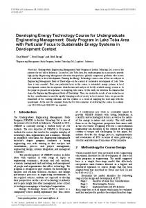
mechanisms to enable or facilitate intelligent behavior in complex, uncertain and changing environments. These adaptive mechanisms include those AI paradigms that exhibit an ability to learn or adapt to new situations, to generalize, abstract, discover and associate. The four dominant computational intelligence paradigms are neural networks, evolutionary computing, swarm intelligence and fuzzy systems as illustrated in figure 1.
Neuro-Swarm Systems
Neural Networks
Neuro-Genetic Systems
Evolutionary-Swarm Systems
Evolutionary Computing
Swarm Intelligence
Neuro-Fuzzy Systems
Fuzzy-PSO Systems
Fuzzy Systems Fuzzy-GA Systems
Figure 1: Four main paradigms of CI
These paradigms can be combined to form hybrids as shown in figure 1 resulting in Neuro-Fuzzy systems, Neuro-Swarm systems, Fuzzy-PSO systems, Fuzzy-GA systems, Neuro-Genetic systems, etc. Designs and developments with hybrid algorithms already exist in literature [2, 3, 4]. The following sections describes the five main parts of the Computational Intelligence course taught at the University of Missouri-Rolla as an experimental course in the Spring semester of 2004. These parts are – neural networks, evolutionary computing, swarm intelligence and fuzzy systems. This course is offered at the 300 level which allows both the undergraduate and graduate students to take. The advantage of doing is that the undergraduate students are exposed to these emerging computational intelligence field; and for the graduate students, the course introduces them to four main paradigms and their interest in any of paradigms can be broaden by a full semester on either of the courses - neural networks, fuzzy logic, evolutionary computation, so on, which is offered at the University of Missouri-Rolla. The textbook used in the spring semester is entitled “Computational Intelligence” by A P Engelbrecht [1]. The course was
offered in three departments: Department of Electrical and Computer Engineering, Department of Mechanical Engineering and Department of Engineering Management. Neural Networks In this part, the topics covered include the artificial neuron model; supervised learning neural networks; unsupervised learning neural networks; Radial Basis Function (RBF) networks. The students are introduced to different neural network architectures and the class is focused on feedforward neural networks. The feedforward neural network and the conventional training algorithm known as the backpropagation [5-8] are described below. The incremental and batch training concepts are taught. A feedforward neural network can consist of many layers as shown in figure 2, namely: an input layer, a number of hidden layers and an output layer. The input layer and the hidden layer are connected by synaptic links called weights and likewise the hidden layer and output layer also have connection weights. When more than one hidden layer exists, weights exist between the hidden layers.
INPUT LAYER
x
HIDDEN LAYER W1 , 1
Σ
W1 , 2
W 2 ,1
OUTPUT LAYER V1 , 1
a1
d1 Desired Output V2 , 1
Σ
+
d2
a2
W2 , 2
y-
Σ Error
W 3 ,1
1 (bias)
W4 ,1 W4 , 2
V3 ,1
Σ
W3 , 2
Σ
a3
d3
a4
d4
V 4 ,1
TRAINING ALGORITHM
Figure 2: Feedforward neural network with one hidden layer
Neural networks use some sort of "learning" rule by which the connections weights are determined in order to minimize the error between the neural network output and desired output. The following subsections section the two paths involved in a neural network usage – the forward path and the backward path. The backward is described for the backpropagation training algorithm. (a). Forward path The feedforward path equations for the network in figure 2 with two input neurons, four hidden neurons and one output neuron are given below. The first input is x and the second is a bias input (1). The activation function of all the hidden neurons is given by (1).
ai = Wij X
for i =1 to 4, j = 1, 2 (1)
x
where Wij is the weight and X = is an input vector. 1
The hidden layer output called the decision vector d is calculated as follows for sigmoidal functions: di =
1 1 − e(
ai )
for i =1 to 4 (2)
The output of neural network y is determined as follows: d1 d y = [V1 , V 2 , V 3 , V 4 ] 2 d3 d 4
(3) (b). Backward path with the conventional backpropagation The serious constraint of the backpropagation algorithm is that the function approximated should be differentiable. If the inputs and desired outputs of a function are known then backpropagation can be used to determine weights of the neural network by minimizing the error over a number of iterations. The weight update equations of all the layers (input, hidden, output) in the multilayer perceptron neural network are almost similar, except that they differ in the way the local error for each neuron is computed. The error for the output layer is the difference between the desired output (target) and actual output of the neural network. Similarly, the errors for the neurons in the hidden layer are the difference between their desired outputs and their actual outputs. In a MLP neural network, the desired outputs of the neurons in the hidden layer cannot be known and hence the error of the output layer is backpropagated and sensitivities of the neurons in the hidden layers are calculated. The learning rate is an important factor in the backpropagation algorithm. If it is too low, the network learns very slowly and if it is too high, then the weights and the objective function will diverge. So an optimum value should be chosen to ensure global convergence which tends to be difficult task to achieve. A variable learning rate will do better if there are many local and global optima for the objective function. Backpropagation equations are explained in more detail in [5] and they are briefly described below. The output error ey is calculated as the difference between the desired output vector yd and actual output y.
e y = yd − y
(4) The decision error vector ed is calculated by backpropagating the output error ey through weight matrix V. edi = ViT ey
for i =1 to 4 (5)
The activation function errors are given by the product of decision error vector edi and the derivatives of the decision vector di with respect to the activations ai. eai = di (1 − di )edi
(6) The changes in the weights are calculated as ΔV (k ) = γ m ΔV (k − 1) + γ g ey d T
(7a) ΔW (k ) = γ m ΔW (k − 1) + γ g ea X
T
(7b) where γ m is a momentum term, γ g is the learning gain and k is the iteration/epoch number. A momentum term produces a filter effect in order to reduce abrupt gradient changes thus aiding learning. Finally the weight update equations are below. W (k + 1) = W (k ) + ΔW (k )
(8a) V (k + 1) = V (k ) + ΔV (k )
(8b) The learning gain and momentum term have to be carefully selected to maximize accuracy, reduce training time and ensure global minimum. A JAVA based software developed for MLP neural networks developed by the author is used to teach the need to carefully select these parameters and their effects [9]. Evolutionary Computation (EC) In this part, the topics covered include Genetic Algorithms (GAs), Genetic Programming (GP), Evolutionary Programming (EP), Evolutionary Strategies (ESs). These algorithms are introduced and their numerous applications are demonstrated in class through examples. The differences between these algorithms, when and where these algorithms are applicable is emphasized in class. The main steps in EC algorithms are given below. • Initialize the initial generation of individuals.
•
While not converged i) Evaluate the fitness of each individual ii) Select parents from the population iii) Recombine selected parents using crossover to get offspring iv) Mutate offspring v) Select new generation of populations
Swarm Intelligence In this part, the topics covered include Particle Swarm Optimization (PSO), Ant Colony Optimization, Cultural and Differential Evolution. These algorithms are introduced and their numerous applications are demonstrated in class through examples. The differences between these algorithms, when and where these algorithms are applicable is emphasized in class. Emphasis is given the PSO algorithm and taught in detail. The PSO algorithm is described below. Particle swarm optimization is an evolutionary computation technique (a search method based on natural systems) developed by Kennedy and Eberhart [10, 11]. PSO like a generic algorithm (GA) is a population (swarm) based optimization tool. However, unlike GA, PSO has no evolution operators such as crossover and mutation and more over PSO has less number of parameters. PSO is the only evolutionary algorithm that does not implement survival of the fittest and unlike other evolutionary algorithms where evolutionary operator is manipulated, the velocity is dynamically adjusted. The system initially has a population of random solutions. Each potential solution, called particle, is given a random velocity and is flown through the problem space. The particles have memory and each particle keeps track of previous best position and corresponding fitness. The previous best value is called as ‘pbest’. Thus, pbest is related only to a particular particle. It also has another value called ‘gbest’, which is the best value of all the particles pbest in the swarm. The basic concept of PSO technique lies in accelerating each particle towards its pbest and the gbest locations at each time step. Acceleration has random weights for both pbest and gbest locations. Figure 3 illustrates briefly the concept of PSO, where Xk is current position, Xk+1 is modified position, Vini is initial velocity, Vmod is modified velocity, Vpbest is velocity considering pbest and Vgbest is velocity considering gbest.
Y
Xk+1 Vmod
t Vgbest
s Vpbest Xk
r Vini X
Figure 3: Position update of a PSO particle (r, s and t are some constants)
i) Initialize a population (array) of particles with random positions and velocities of d dimensions in the problem space. ii) For each particle, evaluate the desired optimization fitness function in d variables. iii) Compare particle’s fitness evaluation with particle’s pbest. If current value is better than pbest, then set pbest value equal to the current value and the pbest location equal to the current location in d-dimensional space. iv) Compare fitness evaluation with the population’s overall previous best. It the current value is better than gbest, then reset gbest to the current particle’s array index and value. v) Change the velocity and position of the particle according to (9) and (10) respectively. Vid and Xid represent the velocity and position of ith particle with d dimensions respectively and, rand1 and rand2 are two uniform random functions. Vid = w × Vid + c1 × rand 1 × ( Pbestid − X id ) + c 2 × rand 2 × ( Gbestid − X id )
(9) X id = X id + Vid
(10) vi) Repeat step ii) until a criterion is met, usually a sufficiently good fitness or a maximum number of iterations/epochs. PSO has many parameters and these are described as follows: w called the inertia weight controls the exploration and exploitation of the search space because it dynamically adjusts velocity. Local minima are avoided by small local neighborhood, but faster convergence is obtained by larger global neighborhood and in general, global neighborhood is preferred. Synchronous updates are more costly than the asynchronous updates. Vmax is the maximum allowable velocity for the particles i.e. in case the velocity of the particle exceeds Vmax then it is reduced to Vmax. Thus, resolution and fitness of search depends on Vmax. If Vmax is too high, then particles will move beyond good solution and if Vmax is too low, then particles will be trapped in local minima. c1, c2 termed as cognition and social components respectively are the acceleration constants which changes the velocity of a particle towards pbest
and gbest (generally somewhere between pbest and gbest). Velocity determines the tension in the system. A swarm of particles can be used locally or globally in a search space. In the local version of the PSO, the gbest is replaced by the lbest and the entire procedure is same. More details and results are given in [2]. Fuzzy Logic In this part, the topics covered include Fuzzy Systems, Fuzzy Interference Systems, Fuzzy Controllers, Rough Sets. The design of a fuzzy room temperature controller and fuzzy cruise controller is taught in a step by step fashion through fuzzification process, interference engine, rule set and defuzzication process is carried out in class. Hybrid Algorithms In this part, the students train a feedforward neural network using GA, ES and PSO algorithms, and compare the training results with that of the backpropagation algorithm. In addition, they do a survey of neuro-fuzzy controllers and write a report on how fuzzy memberships can be used within a neural network structure. Course Assessment The course assessment is made of: • 25% Homework/Assignments • 25% Midterm Exam • 40% Group Project Report • 5% Class presentation • 5% Quizzes The course grading is based on six homeworks where they have to write MATLAB programs to train feedforward neural networks with the backpropagation algorithms, GA, ES and PSO, train a learning vector quantization (LVQ) network using competitive learning and the last one write a report on neuro-fuzzy structures. Projects are carried out involving at least two of four CI paradigms and done in groups. Each group is made of four students. The students are encouraged to start early in the semester. Conclusion The students that took class consisted of two undergraduates and ten graduate students (MS and PhD). The feedback received from students is mainly the great exposure to the different paradigms of computational intelligence in a semester. One of the undergraduate students who took the class in Spring 2004 is currently doing research in the area of evolvable hardware and had his publication in Fall semester of 2004 [12]. The other undergraduate is interested in doing a MS degree in the area of computational intelligence. All the graduate students who took the course are pursuing a thesis involving components of computational intelligence. The offering of the CI experimental course at the 300 level allowing both undergraduate and graduate students
has been a successful effort. It is anticipated the experimental course will be offered once more in the Fall semester of 2005 and thereafter made a permanent course in the Electrical Engineering and Computer Engineering Curriculum at the University of Missouri-Rolla. References [1]. A. Engelbrecht, Computational Intelligence: An Introduction, John Wiley & Sons, Ltd, England. ISBN 0-47084870-7. [2]. V. G. Gudise, G. K. Venayagamoorthy, “Comparison of particle swarm optimization and backpropagation as training algorithms for neural networks”, IEEE Swarm Intelligence Symposium, Indianapolis, IN, USA, April 24 -26, 2003, pp.110 - 117. [3]. G. K. Venayagamoorthy, “Adaptive critics for dynamic particle swarm optimization”, IEEE International Symposium on Intelligent Control, September 2 – 5, 2004, Taipei, Taiwan, pp. 380 -384. [4]. X. Cai X, N. Zhang, G. K. Venayagamoorthy, D. C. Wunsch, “Time series prediction with recurrent neural networks using a hybrid PSO-EA algorithm”, IEEE-INNS International Joint Conference on Neural Networks, Budapest, Hungary, July 24 -29, 2004. [5]. S Haykin, Neural networks: A comprehensive foundation, Prentice Hall, 1998, ISBN 0-1327-3350-1. [6]. P. J. Werbos, "Backpropagation through time: what it does and how to do it". Proceedings of the IEEE, Vol: 78:10, Page(s): 1550 –1560, Oct. 1990. [7]. P. J. Werbos, The roots of backpropagation, New York: Wiley, 1994. [8]. D. E.Rumelhart, G. E. Hinton and R. J. Williams, "Learning representations by back-propagating errors", Nature, Vol.323, pp.533-6, 1986. [9]. G.K. Venayagamoorthy, “Teaching Neural Networks Concepts and their Learning Techniques”, 39th ASEE Midwest Section Meeting, Pittsburg, Kansas, September 29 to October 1, 2004. [10] J. Kennedy and R. Eberhart, "Particle swarm optimization", Proceedings of IEEE International Conference on Neural Networks, Perth, Australia. Vol. IV, pp. 1942–1948. [11] J. Kennedy and R. C. Eberhart, Swarm intelligence, Morgan Kaufmann Publishers, 2001. [12] P. Moore, G.K. Venayagamoorthy, “Evolving Digital Circuits Using Hybrid Particle Swarm Optimization and Differential Evolution”, Conference on Neuro-Computing and Evolving Intelligence, Auckland, New Zealand, December 13 – 15, 2004, pp. 71 -73.
Acknowledgment The support from the National Science Foundation under CAREER Grant: ECS # 0348221 is gratefully acknowledged for this work. The author is grateful for the following departments at the University of Missouri-Rolla for offering the experimental course on computational intelligence to their students: Electrical and Computer Engineering, Mechanical Engineering and Engineering Management.
Biography Ganesh Kumar Venayagamoorthy received the B.Eng. (Honors) degree with a first class in electrical and electronics engineering from the Abubakar Tafawa Balewa University, Bauchi, Nigeria, and the M.Sc.Eng. and Ph.D. degrees in electrical engineering from the University of Natal, Durban, South Africa, in March 1994, April 1999 and February 2002, respectively. He was appointed as a Lecturer with the Durban Institute of Technology, South Africa during the period March 1996 to April 2001 and thereafter as a Senior Lecturer from May 2001 to April 2002. He was a Research Associate at the Texas Tech University, USA in 1999 and at the University of
Missouri-Rolla, USA in 2000/2001. He joined the University of Missouri-Rolla, USA as an Assistant Professor in May 2002. His research interests are in computational intelligence, power systems, control systems and digital systems. He has authored about 100 papers in refereed journals and international conferences. Dr. Venayagamoorthy is a 2004 National Science Foundation, USA CAREER award recipient, the 2003 International Neural Network Society Young Investigator award recipient, a 2001 recipient of the IEEE Neural Network Society summer research scholarship and the recipient of five prize papers with the IEEE Industry Application Society and IEEE Neural Network Society. He is a Senior Member of the Institute of Electrical and Electronics Engineer (IEEE), USA, and South African Institute of Electrical Engineers (SAIEE). He was Technical Program Co-Chair of the International Joint Conference on Neural Networks (IJCNN), Portland, OR, USA, July 20 – 24, 2003 and the International Conference on Intelligent Sensing and Information Processing (ICISIP), Chennai, India, January 4 – 7, 2004. He is founder and currently the Chair of IEEE St. Louis Computational Intelligence Society Chapter.