Development of a Decision Support Tool for Kenya's ... - CiteSeerX

AURA ET AL

37

Development of a Decision Support Tool for Kenya’s Coastal Management Stella Aura1, Charlies Ngunjiri2, Johnson Maina1, Paul Oloo1, John Muthama3 (1) Kenya Meteorological Department; E-mail: [email protected] (2)Ministry of the East African Community (3)Department of Meteorology, University of Nairobi, Kenya

ABSTRACT Coastal management is crical in view of the danger posed to coastal communies by flooding from the sea due to storm surges, sea-level rise and Tsunamis. The low-lying Kenyan coast is vulnerable to these hazards, therefore modeling their effects is necessary for understanding their socio-economic impacts. A Decision Support Tool (DST) was developed to study the hydrodynamics along the Kenyan coast. The bathymetry grid for the DST was created using Arc View GIS from naucal charts. MIKE 21 Hydrodynamic Module (HD) Demo version was used to organize the bathymetry and enforce boundary condions for ELCOM simulaon. Tidal data was obtained from both the Kenya Meteorological Department’s dal gauges and the GLOSS staon. The computed de and currents from ELCOM were validated using graphical and stascal comparison. Their predicve ability was analyzed. The ELCOM water levels and currents compared well to observed values, and their dominant signals were detectable. ELCOM could, therefore, simulate and forecast coastal hydrodynamics. This DST can assist the Government in operaonal forecasng for marine environmental protecon, resources management and disaster risk reducon and migaon as well as infrastructure mapping and development along the Kenyan coast. Keywords: Coastal flooding, ELCOM, MIKE 21, Marine environmental management, Disaster risk reducon, Kenyan coast

1. Introduc!on The Kenyan coast, which is about 600 km long and runs in a southwesterly direcon from the border with Somalia in the north to Tanzania in the south, has been shaped by forces of the sea. The semi-annual reversal of monsoon winds, caused by large scale pressure changes over southwestern Indian Ocean and the vast Asian land mass, influences the ocean currents off Kenya. These currents are dominated by the East African coastal current (EACC). Kenyan coastal waters are characterized by semi-diurnal des with spring and neap dal variaons of about 4.0 and 1.8 m respecvely (Rao & Ram, 2005; Tychsen, 2006; Quinn et al., 2007; GoK, 2009). The coastal ecosystem which includes, coral reefs, sea grass beds, mangroves, sandy beaches and dunes, naturally buffer the coast against flooding. They protect beaches against erosion and barrier the coastline against storm surges, waves and Tsunamis through their ability to dissipate wave energy. They therefore provide essenal ecological services and livelihood, and generate income for coastal

and inland populaons, but face the highest threat in the world. Conservaon of the ecosystem is essenal for socio-economic development (Tychsen, 2006; GoK, 2009). Coastal management is important in view of the danger posed to coastal communies due to coastal flooding caused by storm surges, sea level rise and Tsunamis (ICAM, 2009). Storm surges induced by tropical cyclones (TCs), which occur over southwestern Indian Ocean, have indirect effects along the Kenyan coast, but their predicon is important for coastal disaster planning and migaon (Gönnert et al., 2001; Resio & Westerin, 2008). The global sea level is currently rising by about 4 mm per year (IPCC, 2007). A sea level rise of about 0.3 m is likely to submerge close to 17% of Kenya’s coastland, which lies up to 10 m above mean sea level (MSL). The ability to develop marine products will reduce sea-level rise uncertaines, improve coping mechanisms and contribute in idenfying vulnerable areas (Nicholls et al., 2007; Awuor et al., 2008;

KMS 10th CONFERENCE SPECIAL ISSUE

38

JOURNAL OF METEOROLOGY AND RELATED SCIENCES

Thompson et al., 2008; UNESCO/IOC, 2010). A large part of the Kenyan coast was affected by the 26 December 2004 Sumatra Tsunami (IOC, 2008). The Kenya Meteorological Department (KMD) installed Tsunami monitoring systems along the coast to monitor and mi"gate against future Tsunamis and other marine hazards. However, there is lack of sufficient numerical modeling skills and manpower. Hydrodynamic models will improve forecasts of future Tsunami scenarios and will fill some of the missing gaps in the exis"ng KMD Tsunami project (UNESCO, 2009). The low-lying Kenyan coastline and its shallow sea are vulnerable to flooding from the sea, with the risk of loss of life and property (Awuor et al. 2008; GoK, 2009). Coastal flooding leads to habitat loss, erodes beaches, renders land uninhabitable and reduces the natural buffering ac"on against storm surges, waves, Tsunamis and shoreline erosion. Li&le or no effort had been done to monitor and understand Coastal hydrodynamics (Quinn et al., 2007; Awuor et al., 2008; GoK, 2009). Therefore, there was need to iden"fy tools, to evaluate and predict the risk of floods in coastal areas. Numerical modeling allows these natural events to be understood so that lives and property can be protected (Massey et al. 2007; ICAM, 2009). KMD partnered with UNESCO/IOC to develop a hydrodynamic DST using the Estuary Lake and Coastal Ocean Model (ELCOM), This DST will assist the Government and stakeholders in decision-making in the areas of forecasting for marine environmental protec"on, resources management, disaster risk reduc"on and mi"ga"on as well as infrastructure mapping and development along the Kenyan coast.

iii. iv.

MIKE 21 for input into ELCOM. Carrying out hydrodynamic simula"ons us ing ELCOM to develop model outputs. Valida"on of model outputs and analysis of predic"ve ability of ELCOM.

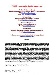
2.0 Materials and Methods 2.1 Materials The study area which was along the Kenyan coast is shown in Figure 1. It also shows the hydrodynamic area of interest, within Lamu (2°15’S, 40°54’E) and Kilifi (3°36’S, 39° 51’E). The bathymetry, "dal and current meter datasets were used in this study. The bathymetry data were obtained from the United Kingdom Hydrographic Office (UKHO) nau"cal charts 3361 and 238. Chart 3361 covered the region between Pemba Island and Lamu had a coarse resolu"on of 3.5 km, while the finer chart 238 with resolu"on of 375 and 250 m covered Malindi and Kilifi areas, respec"vely.

1.1 Objecves The overall objec"ve of the study was to develop an opera"onal forecas"ng tool (DST) for marine environmental protec"on, resources management and disaster mi"ga- Fig. 1. The Kenyan coastline and the Area of interest in the study "on. This would be achieved through simula"ons of coastal inunda"on scenarios for storm surges, Tidal gauge data, required for open boundary forcing sea-level rise and Tsunamis. The specific objec"ves and model valida"on within ELCOM simula"on, was included: available from the Kilifi Meteorological sta"on and i. Crea"on of bathymetry grid from nau"cal Lamu Global Sea-Level Observa"on System (GLOSS) charts using ArcView GIS. "de gauges. The Lamu GLOSS gauge has operated ii. Organiza"on of bathymetry and "dal data in since 1995 while the Kilifi gauge was installed in KMS 10th CONFERENCE SPECIAL ISSUE

AURA ET AL

2007. The hourly values for the period May 2008 to May 2009 were used, for consistency purposes. The surface ocean current data were collected at Malindi around Kipini/Ungwana Bay for a ten-day period on 11 – 22 August 2008, and in August 2009. The current speed and direcon were sampled at 15-minutes me interval for model validaon. 2.2 Bathymetry Set-Up ArcView GIS facilitated the mapping and characterizaon of sensive coastal and ocean floor environments. The mapping of spaal informaon enhances the use and management of earth’s resources (Zeiler, 1999). The scanned maps of the UKHO Naucal Charts 3361 and 238 were separately geo-referenced into the geographic coordinate system of latude/longitude using ArcView GIS 3.2a. A reference system was chosen for aligning the geo-referenced naucal charts to the earth’s spaal features. The coastline bathymetry informaon, the fundamental geophysical data for hydrodynamic modeling process, were extracted through digizaon to create different Geographic Informaon System (GIS) layers in terms of points, polygons and vector shape files (ESRI, 2001). The bathymetry layers were transformed into Cartesian coordinate system for data input in MIKE 21 and ELCOM. Therefore, the GIS layers were re-projected from geographic to the projected coordinate system based on Universal Transverse Mercator (UTM) zone for Kenyan coast. The different GIS layers were combined into point GIS layers for interpolaon purposes. An appropriate spaal interpolaon tool was selected from the Spaal Analyst extension of ArcGIS for creating the bathymetry grid from the point layers (Zeiler, 1999). The created bathymetry grid was fed into MIKE 21. 2.3 Model Inialisaon In this study, MIKE 21 Hydrodynamic Module (HD) Demo version was used to organize the bathymetry data into proper format and enforce boundary condions using Kilifi and Lamu des, the main water forcing for ELCOM (DHI, 2005; DHI, 2007). The stability of ELCOM depended on the grid resoluon; the computaonal points were therefore set in rectangular grid in MIKE 21. The rectangular model grid was rotated to align the grid parallel to one of the coordinate axes for conservaon of mass and momentum in ELCOM. The open boundaries were located in regions that did not

39

dry out. The bathymetry grids were recfied in MIKE 21 using the bilinear interpolaon tool to remove irregular points which remained aer interpolaon in ArcView GIS. The interpolaon also included and excluded computaonal areas which somemes flooded or dried out (Hodges and Dallimore, 2006). The bathymetry data were referenced to the depths on sea charts by the lowest astronomical de (LAT) which represented the MSL. The digized bathymetries were related to the reference datum as defined in ArcView GIS. True land values were the minimum values specified for land points during bathymetry preparaon. Open boundary values were the values much higher than the minimum land points which were the open boundary points for bathymetry preparaon in MIKE 21. The Kilifi and Lamu water level data were converted using LAT which represented MSL. Their dal datum was determined using the annual average value. Their dal values, the main boundary forcing, were used to define the free surface posion at every me step, for intermediate points along the model boundaries, through linear interpolaon in MIKE 21. The MIKE 21 demo version had limited simulaon capability, therefore hydrodynamic simulaon was done using ELCOM model. 2.4 Hydrodynamic Model Simulaon Using ELCOM ELCOM, a 3D model, simulates the temporal behavior of strafied water bodies by applying the hydrodynamic and thermodynamic codes using the hydrostatic and Boussinesq assumpons (Hodges and Dallimore, 2006). The ELCOM outputs characterize water movement and mixing in water bodies, and therefore help to understand coastal hydrodynamics. ELCOM has been applied to model lakes and other water bodies in various locaons around the world with great success (Hodges et al., 2000; Laval et al., 2003; Appt et al., 2004; Leon et al., 2005). ELCOM was chosen for the Kenyan Coast based on its proven accuracy, ability to run on a personal computer, and abundance of documentaon. The bathymetry data were exported from MIKE 21 into ELCOM for the simulaon. The horizontal grid resoluon was set up with constant spacing to improve ELCOM runs. Non-uniform vercal grids were also created. The open boundary forcing for ELCOM were the Kilifi and Lamu des. The ELCOM simulaon was restricted to the period during which data for forcing and validang model outputs were available.


40


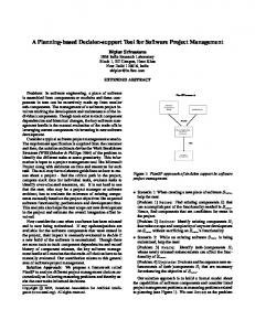
In order to avoid instability at the first me steps of the simulaon, the inial surface elevaon were matched with the boundary condion at the first me step. The inial values for wind, temperature and salinity were specified; they were found to match local coastal physics. The effect of the earth’s rotaon, thermodynamic process, turbulence and boom drag coefficient were also taken into account. The me step which considered the Courant-Fredrich-Lewy (CFL) condion for the stability of the simulaons was specified. The total number of me steps was determined by the required model outputs. ELCOM calculated at each grid point and for each me step the water levels, flux densies and water velocies. In this study, the main outputs were the synopc images of water levels and the current speed and direcon at different me steps. 2.5 Model Validaon In this study, the quantave assessment of the model performance was mainly based on the graphical and stascal comparison of model outputs and observaon samples. Simulated results were extracted that corresponded to the same locaon, date and me as the observaons, for the sake of compariFig. 2. The digised bathymetry grid represenng land and water son to gauge the validity of ELCOM outputs. points along the Kenyan Coastline. The ability of the model to reproduce field measurements was further evaluated by assessing to WGS84 datum, the coastline geographical and bathe model fit using a 1:1 regression line (Zhang et al., thymetry digital data were extracted in GIS layers of 2006). This technique avoids bias from consistent un- point and contours shape files which represented der- or over-predicon of simulated values (Spillman land and depth sounding. All land contours and elet al., 2007). The computed dal and current outputs evaons with MSL ≥ 10 m contour line represented were also analyzed using Fourier analysis to test the land points and were specified by 10 m, for purposes predicve capacity of ELCOM to reproduce dominant of se#ng up the bathymetry. The low de mark contour on the naucal charts was specified by zero (0) signals in des and currents (Bloomfield, 2000). m contour line, which was the LAT. All land contours and elevaons, 0 < MSL < 10 m contour line, with their 3.0 Results and Discussion specified values, which were the drying and we#ng areas in MIKE 21, were used to demarcate land and 3.1 Bathymetry Set-Up The naucal charts were geo-referenced to geograph- sea boundary. All other values below MSL were negaic coordinates of decimal degrees in ArcMap. The ve and represented water points. The digized GIS layers were transformed using World Geodec System of 1984 (WGS84) datum was used to align the geo-referenced map to the features the ArcView projecon ulity from the geographic on the earth’s surface. The origin of WGS84 ellipsoid coordinate system in decimal degrees to the WGS84 is at the earth’s center of mass; this datum minimized UTM zone 37S in metres, the appropriate UTM zone map distorons. A!er registering the charts features for Kenyan coast which ensured minimum spaal disKMS 10th CONFERENCE SPECIAL ISSUE

AURA ET AL

41

that mass and momentum were conserved in the domain region (DHI, 2005; Hodges and Dallimore 2006). The bathymetry grid was smoothened using bilinear interpolaon at all open and closed boundaries to produce well behaved flows. The interpolaon produced slowly varying water depths hence catered for flooding and drying areas which were made not completely level but given a gentle slope towards the nearest area with deep water. This ensured that a series of dry pond points were not le$ in the otherwise dry areas when the water withdraws (DHI, 2005; DHI ,2007). The reference level in this study, the MSL, was taken as 0.3m, which was the LAT and the bathymetry and water levels were related to the LAT which was based on WGS84 datum. The land boundary value was specified by 10 m, which represented land points, while the open boundary points for water was specified by 888 m. Kilifi and Lamu des were separated by about 300 km distance which was sufficient for modeling purposes. The enforced water boundaries ensured conservaon of mass with mass inflow and outflow at Kilifi and Lamu respecvely, hence Fig. 3. The region of interest and rotated rectangular domain a$er imporng the land and water point bathymetry data into MIKE 21. connuity could be preserved at the computaonal grid during the flooding and drying process. The domain horizontal extension toron and visual interpretaon of distances. The dig- was 62.5 by 180 km, in x- and y-direcon respecvely, ital land/water point and contours were all converted giving a total of 45,000 water points that were includto point GIS layers for the interpolaon process. The ed in the hydrodynamic computaon for ELCOM. The Inverse Distance Weighted (IDW) spaal interpolaon bathymetry grid which was created in MIKE 21 and tool was used to create the necessary bathymetry used for ELCOM simulaon is shown in Figure 4. grid using the land/water points. Figure 2 shows the digized bathymetry grid of the Kenyan coastline pro- 3.3 Model Simulaon Outputs Using Elcom duced using ArcView GIS 3.2a. The derived bathym- The rectangular horizontal grid set-up in MIKE 21 caetry grid provided beer insights for further analysis. tered for enhanced performance of ELCOM runs. The set-up of bathymetry layers in the vercal was slowly varied to enhance ELCOM accuracy by se&ng up 18 3.2 Model Inialisaon The bathymetry was set up in a rectangular domain non-uniform grids (Hodges and Dallimore, 2006). The with horizontal grid resoluon of 500 m in MIKE 21 as open boundary forcing for ELCOM were the water shown in Figure 3. This would ensure beer perfor- level variaons as defined in MIKE 21. ELCOM simumance and stability of ELCOM simulaons. The model laons were carried out using data for August 2008 area was rotated clockwise by 20° with Kilifi and Lamu due to unavailability of necessary datasets for model as the southern and northern boundaries respecve- validaon. The model domain captured the low lying ly, this ensured that domain area was oriented par- region of Ungwana Bay around Malindi and the outlet allel with the coast. The rotaon necessitated water of rivers Tana and Athi-Sabaki into the Indian Ocean. inflow at Kilifi and ou#low at Lamu, which guaranteed Freshwater inflow data from the two major rivers KMS 10th CONFERENCE SPECIAL ISSUE

42


were not considered although they play some role in density mixing along the estuary. The inial surface elevaon of 0.5 m was used since the model inialized the fluxes and current velocies to zero. The inial surface elevaon matched the boundary condion at the first me step. This allowed the model to obtain stable soluons faster. Inial wind speed was set to 10 m/sec. Water temperature and salinity was inialized based on the heat balance equaon, with inial values of 24o C and 35% respecvely. The earth’s rotaon was accounted for by varying the Coriolis force in space, but not in me. The thermodynamic roune controlled the heat transfer which affected air temperature, humidity and water clarity. The effect of turbulence and momentum caused by turbulence on water velocity was considered by the turbulent benthic boundary layer. The boom resistance was factored by the boom drag of 0.005. The ELCOM outputs from water level as high de was approached at 1800 hrs on 11 August 2008 show that high water levels of more than 0.8 m overlies Lamu and Kilifi regions as compared to Malindi which has lower value of less than 0.8 m (Figure 5). The situaon appeared to be reversed as the water level recedes because higher waters overlie Malindi in comparison to the other two areas (Figure 5). The bathymetry, coastal dynamics, the fast flowing EACC and meteorological factors over these regions might play a significant role in the inundaon of the coastal areas (Rao & Ram 2005; Tychsen, 2006). The current speed outputs during the period (as Fig. 4. Bathymetry of the model domain created in MIKE21 high and low water marks are approached) shows that the current speeds are strong towards the south, close hydrodynamic module for ELCOM simulaon.

Fig. 5. Water level model output over the domain region at 1630, 1700 and 1730 as high water (le! three) and at 2230, 2300 and 2330 as low de (right three) is approached on 11 August 2008.


AURA ET AL

43

Fig.6: Current speed model output over the domain region at 1630, 1700 and 1730 as high water (le! three) and at 2230, 2300 and 2330 as low de (right three) is approached on 11 August 2008.

Fig. 7. Current direcon model output over the domain region at 1630, 1700 and 1730 as high water (le! three) and at 2230, 2300 and 2330 as low de (right three) is approached on 11 August 2008.

to Kilifi, as compared to other areas (Figure 6). This may be aributed to the faster flowing EACC which is forced by the SEM and possibly the East African Low Level jetstreams, which overly these areas during the month of August (Rao & Ram, 2005; Tychsen, 2006). The daily variaons in the current speeds may also be due to small-scale eddies generated by the currents and freshwater inflows from rivers Tana and Athi respecvely. The current speeds are generally closer to the coastline, with slight increase away from the near-shore regions. Figure 7 shows that the dominant current direcon was northerly, mainly forced by the northward flowing EACC (Tychsen, 2006). 3.4 Model Validaon The ELCOM validaon was based on the period 11 – 22 August 2008, during which dal and current meter

datasets were available. Figure 8 depicted the plots of the actual and simulated water level data at Kilifi and Lamu. The graphical comparison showed that the numerical results agreed well with the observaons at both Kilifi and Lamu, providing confidence that the model could well reproduce the dal flows. Figure 9 depicted the plot of the observed and computed current speeds and direcon at Malindi. The validaon generally showed that the model reproduced current speeds which were comparable to the sampled measurements. The computed current speeds captured the diurnal variaons with two high and low values, which are forced by the dal variaons. The computed current direcons were somemes observed to be out of phase with the actual measurements, while the calculated currents appeared to capture the climatology of ocean currents


44


Kilifi Tidal Data (Observed vs Model Data) 1.5

observation

Lamu Tidal Data (Observed vs Model Data)

model observation

1.3

model

1

18-Aug-08

17-Aug-08

16-Aug-08

15-Aug-08

14-Aug-08

13-Aug-08

-0.2

12-Aug-08

18-Aug-08

17-Aug-08

16-Aug-08

15-Aug-08

14-Aug-08

13-Aug-08

-0.5

12-Aug-08

0

0.3

11-Aug-08

Tidal Elevation (metres)

0.5

11-Aug-08

Tidal Elevation (metres)

0.8

-0.7

-1

-1.2

Date of the Year

Date of the Year -1.7

-1.5

Fig. 8. The actual and simulated water level data at Kilifi (le!) and Lamu (right).

Malindi Current Direction (Observed vs Model Data)

Malindi Current speed (Observed vs Model Data)

0.4

observation

model

observation

360

model

0.35 300

Direction (Deg)

0.25 0.2 0.15

240

180

120

0.1 60

0.05 0

18-Aug-08

17-Aug-08

16-Aug-08

15-Aug-08

14-Aug-08

13-Aug-08

12-Aug-08

18-Aug-08

17-Aug-08

16-Aug-08

15-Aug-08

14-Aug-08

13-Aug-08

12-Aug-08

11-Aug-08

0

11-Aug-08

Speed (metres/sec)

0.3

Date of the year

Date of the Year

Fig. 9. The actual and simulated current speeds (le!) and direcon (right) at Malindi.

direcon (Tychsen, 2006). The model skill of the Kilifi and Lamu des and Malindi current speed based on the scaer plot fit to the regression line are shown in Figure 10. Again, generally good agreement could be observed, especially the dal flows at Lamu, which showed beer fit with a value of 0.994, which is fairly close to 1. This indicated that the simulated data points were close to the 1:1 regression line (Spillman et al., 2007). Lamu’s rootmean-square error was shown to be 7.4%. The dal flows at Kilifi showed beer fit towards high des as compared to low des. The scaer plot gave a model fit of 0.987 with root-mean-square error of 11.2%. The computed dal flows accurately reproduced the observed condions. In general, good agreement could be observed for the current speeds at Malindi, whose scaer plot

accounted for more than 97.06% of the variance. The root-mean-square error of the speed was slightly lower at 17.9%. The computed current speeds could reproduce the observed condions. The capability of ELCOM to reproduce the dominant signals from the computed Kilifi and Lamu des as well as Malindi current speeds are given in Figure 11. The computed dal data at Kilifi and Lamu show a major frequency at 11 hours, with a minor frequency at 12 hours. These dal frequencies basically show the major influence of the moon and the sun in the des. The frequencies are centred at 11, 12, 6, 10 and 1 hour in descending order of magnitudes for both Kilifi and Lamu. The current speeds at Malindi are mainly forced by a major and minor frequencies centred at ½ and 5½ hours respecvely. The current variaons may be


AURA ET AL

Model Skill of Kilifi Tidal outputs

0.4

-0.2

-0.8

-0.3

0.3

0.9

Observed Tidal Level (metres)

1.5

Model Current speed (m/sec)

Model Tidal Level (metres)

Model Tidal Level (metres)

1.0

-0.8

Model Skill of Malindi Current Speed Output

Model Skill of Lamu Tidal output

1.6

-1.4-1.4

45

1 1 0 -0 -1 -2-1.6

-1.0

-0.4

0.2

0.9

1.5

0.4

0.3

0.2

0.1

0.1

0.00.0

Observed Tidal Level (metres)

0.1

0.1

0.2

0.3

0.3

Model Current speed (m/sec)

Fig. 10. The Model skill of the Kilifi (le$) and Lamu (centre) des and Malindi current speeds (right).

Fig. 11. The Fourier analysis of computed dal outputs at Kilifi (le$) and Lamu (centre) and current speed outputs at Malindi.

forced by the effect of the moon due to rising and receding des, including cyclical variaons with a period of half an hour. In general, Fourier analysis shows that the des and currents may be predicted using the ELCOM Model since it could produce the dominant signals that drive the des and currents. 4. Conclusion The accuracy of ELCOM simulaons suggest that the model is capable of describing and predicng the circulaon pa!erns along the coastline, using various meteorological and oceanographic forces. Although only dal forcing was ulized, future simulaons would consider other boundary forcing like wind, air and water temperature, salinity, freshwater inflow among other parameters for improved accuracy of the results. Therefore, higher resoluon bathymetry, coastal topography and digital elevaon data would be necessary inputs for the simulaon to improve ac-

curacy of the model outputs. The model products need to be sasfactorily validated before they can be disseminated to the stakeholders. It is therefore important to have field observaons to force and validate the model. In order to achieve be!er simulaon results, it is necessary to enhance real-me oceanographic data acquision through installaon of necessary equipments along the Kenyan coastline. The MIKE 21 HD Demo version that was used had limited simulaon capability; there is need to acquire DHI-MIKE 21 licensed version in order to take full advantage of its mulple modules. Although ELCOM is flexible and computaonally-intensive, it lacked data preparaon and organizaon capacity. This DST will assist the Government and stakeholders in decision-making in the areas of forecasng for marine environmental protecon, resources management, disaster risk reducon and migaon as well


46


as infrastructure mapping and development along the Kenyan coast. Indeed, it is already being used in a limited fashion for marine and oceanography forecasng in KMD. Acknowledgements We would like to extend our appreciaon to UNESCO-IOC through Steffano Mazilli for providing funds for data acquision and for funding the two Hydrodynamic Modeling project workshops during December 2008 and September 2009 held in Nairobi and Mombasa respecvely. We appreciate the technical support provided by Mr. Jason Antenucci of the Center for Water Research, University of Western Australia, during both Hydrodynamic Modeling workshops as well as throughout the development of this DST. Finally, we sincerely acknowledge the contribuon from KMD through its Director, who availed both financial and technical support through its staff who collected data and parcipated in the KMD-UNESCO/ IOC Hydrodynamic modeling project.

REFERENCES Appt, J., Imberger, J., and Kobus, H. ,2004: Basin-scale Moon in Strafied Upper Lake Constance, Lim nology and Oceanography, 49, pp. 919-933. Awuor, C.B., Orindi, V.A. and Adwera, A.O., 2008: Climate change and coastal cies: the case of Mombasa, Kenya. Environment and Urban isaon, 20(1), 231-242. Bloomfield, P.,2000: Fourier analysis of me series: An introducon, 2nd ed. New York: John Wiley & Sons. DHI Water and Environment., 2005: MIKE 21 Flow Model, Hydrodynamic Module. Scienfic Documenta on. Danish Hydraulic Instute (DHI. Horsholm, Denmark. DHI Water and Environment. (DHI), 2007: MIKE 21 Flow Model: Hydrodynamic Module. User Guide. DHI Water & Environment(DHI). Horsholm, Denmark. ESRI., 2001: ArcView GIS Version 3.2a So#ware and User Manual. Environmental Systems Research Ins tute (ESRI), Redlands, CA. Gönnert, G., Dube, S.K., Murty, T., Siefert, W., 2001: Global Storm Surges, Die Küste - 63, ISBN 3-80421054-6, 623 pp. Government of Kenya, 2009: State of the Coast Report: Towards Integrated Management of Coastal and Marine Resources in Kenya. Naonal Environ ment Management Authority (NEMA), Nairobi.

88 pp. Hodges, B.R., Imberger, J., Saggio, A. and Winters, K.B., 2000: Modeling basin-scale internal waves in a strafied lake. Limnology and Oceanography, 45(7), 1603-1620. Hodges, B.R., and Dallimore, C., 2006: Estuary, Lake and Coastal Ocean Model: ELCOM v2.2 Science Manual, Centre for Water Research (CWR), University of Western Australia, Nedlands, Western Australia. ICAM, 2009: Hazard Awareness and Risk migaon in Integrated Coastal Area Management, ICAM Dos sier No. 5. (IOC Guides and Manuals No. 50), 141 pp. IOC, 2008: Tsunami, The Great Waves, Revised Edion. Paris, UNESCO, illus. Intergovernmental Oceano graphic Commission (IOC) Brochure 2008-1. 16pp. Available at: h$p://ioc3.unesco.org/ic/ contents.php?id=169. IPCC, 2007: Fourth Assessment Report: Working Group I Report “The Physical Science Basis”. Intergov ernmental Panel on Climate Change. Available at: h$p://www.ipcc.ch/ipccreports/ar4-wg1.htm Laval, B., Imberger, J., Hodges, B. R. and Stocker, R., 2003: Modeling circulaon in lakes: Spaal and tem poral variaons. Limnology and Oceanography, 48(3), 983–994. Leon L.F., Lam D., Schertzer, W., Swayne, D., 2005: Lake and climate models linkage: a 3-D hydrodynamic contribuon. Advances in Geosciences, 4, 57-62. Massey, W.G., Gangai, J.W., Drei-Horgan, E., Slover, K.J., 2007: History of Coastal Inundaon Models. Marine Technology Society Journal Spring 2007, 41, Number 1. Nicholls, R.J., Wong, P.P., Burke$, V.R., Codigno$o, J.O., Hay, J.E., McLean, R.F., Ragoonaden, S. and Woodroffe, C.D., 2007: Coastal systems and lowlying areas. Climate Change 2007: Impacts, Adaptaon and Vulnerability. Contribuon of Work ing Group II to the Fourth Assessment Report of the Intergovernmental Panel on Climate Change, M.L. Parry, O.F. Canziani, J.P. Palukof, P.J. van der Linden and C.E. Hanson, Eds., Cam bridge University Press, Cambridge, UK, 315-356. Quinn, R., Forsythe, W., Breen, C., Boland, D., Lane, P., Omar, A.L., 2007: Process-based models for port evoluon and wreck site formaon at Mombasa, Kenya. Journal of Archaeological Science, 34, 1449-1460. Rao, L.V.G and Ram, P. S., 2005: Upper Ocean Physical processes in the Tropical Indian Ocean. (A monograph prepared under CSIR Emeritus Scienst Scheme) Naonal Instute of Oceanography, Regional Centre, Visakhapatnam. Resio, D.T. and Westerink, J.J., 2008: Modelling the Phys-


AURA ET AL

ics of Storm Surges. Physics Today September 2008 American Instute of Physics, S-0031-92280809-010-8. Spillman, C.M., Imberger, J., Hamilton, D.P., Hipsey, M.R., Romero, J.R., 2007: Modelling the effects of Po River discharge, internal nutrient cycling and hydrodynamics on biogeochemistry of the North ern Adriac Sea. Journal of Marine Systems, 68, 167–200. Thompson, B., Gnanaseelan, C., Parekh, A. and Salvekar, P.S., 2008: North Indian Ocean warming and sea level rise in an OGCM. J. Earth Syst. Sci. 117(2), pp. 169–178. Tychsen, J., 2006: KenSea – Environmental Sensivity Atlas for Coastal area of Kenya, 76 pp. Copen hagen: Geological Survey of Denmark and Green

47

land. (GEUS); ISBN 87-7871-191-6. UNESCO, 2009: Tsunami risk assessment and migaon for the Indian Ocean; knowing your tsunami risk – and what to do about it. IOC Manuals and Guides, 52, Paris, UNESCO. UNESCO/IOC, 2010: Sea-level Rise and Variability – A Summary for Policy Makers. Zeiler, M. 1999: Modeling Our World. The ESRI Guide to Geodatabase Design. Environmental Sys tems Research Instute, Inc. Redlands, California ISBN 1-879102-62-5. Zhang, A-J., Hess, K.W., Wei, E. and Myers, E., 2006: Implementaon of model skill assessment soware for water level and current in dal regions, NOAA Technical Report NOS CS 24, 61 pp.
