DEVELOPMENT OF A FRAMEWORK BASED ON PYFMI FOR ...

Fifth German-Austrian IBPSA Conference RWTH Aachen University

DEVELOPMENT OF A FRAMEWORK BASED ON PYFMI FOR OPTIMIZATION AND FAULT DETECTION G. A. Böhme1 und N. Réhault1 1 Fraunhofer-Institut für Solare Energiesysteme ISE, Freiburg, Germany

ABSTRACT In this article we describe a methodology and a tool chain that allows reusing simulation models for optimization and fault detection during building operation. We illustrate the integration of simulation models, set up in Modelica, in a Python environment using PyFMI. Then, considering as a demonstrator a complex energy supply system for a school campus in Germany, we show first results for the optimization of the ice storage management of that system. Finally, we discuss further applications of the described setup for offline and online fault detection, optimization and predictive control.

INTRODUCTION Simulation models play a crucial role in the planning phase of complex energy supply systems for buildings, as they allow for determining the best options for the sizing and for the choice of control strategies of HVAC systems. Moreover, they provide an estimate of the expected energy consumption of buildings. The use of simulation models is particularly relevant to determine the control strategies and the optimal operation parameters of complex energy supply systems which involve several heat and power sources, storage capacities and varying demand schemes. However, in their real operation, buildings tend not to reach the expected performance estimated by detailed simulation models (Katipamula and Brambley 2005). The reason for the discrepancies between real and simulated operation are mainly due to uncovered optimization potentials in the systems controls and faults in the real operation of buildings. In order to avoid such shortcomings, the models which were developed in the planning phase can be used during the building operation to optimize control strategies and to detect faults at an early stage, thus enabling a more energy efficient operation and a support of maintenance tasks.

There are principally two different approaches for model use during operation: the offline approach conducts optimization and fault detection based on (historic) monitoring data from a given building and does not feed the results back to the building management system (BMS) in an automated way, while the online approach gets current data from the BMS, evaluates those data in real time and feeds the estimated new set values or fault reports back to the BMS. Because of their immediate impact on the building energy system, online routines have to be tested extensively offline before implementation. A convenient framework for testing optimization and fault detection routines offline, using both, simulation models and monitoring data, is the programming language Python in combination with the package PyFMI. For online application of the tested routines, coupling to the BMS is possible, as will be discussed below. This article is structured as follows: First, we describe in detail the integration and application of simulation models (Modelica) in Python. Then, we introduce a specific example, where we illustrate the implementation of control and optimization schemes into the described framework. Then, we briefly present the results of the optimization routine. Finally, we discuss further steps for the specific example and give an outlook for applications of the general framework.

GENERAL FRAMEWORK The integration of simulation models in python is based on the Functional Mockup Interface (FMI), an open standard which was developed in order to facilitate model exchange and co-simulation across different tools (Blochwitz, Otter et al. 2011). Tools, which support the FMI standard, as e.g. Dymola or SimulationX, allow for the export and import of models in terms of Functional Mockup Units (FMUs). An FMU consists of an xml-file containing the model description and C-code or binaries containing the whole model functionality. Importing

- 108 -

Fifth German-Austrian IBPSA Conference RWTH Aachen University

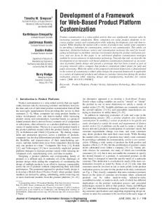
using python routines for offline optimization and fault detection and diagnosis (FDD) on the basis of simulation results and real data from the building. In a further step, the developed and tested Python routines can be connected to the BMS to allow for an online application. Technically, the interaction of the optimization routine with an FMU object model is basically done via the functions model.get(), model.set() and model.do_step(). Figure 2 illustrates the usage of those functions in a simple Python (pseudo) code example. In the following, we introduce an example system, which will serve as a demonstrator to illustrate how the proposed framework can be used for designing and testing optimization routines.

EXAMPLE SYSTEM

Figure 1: Schematic of proposed framework an FMU into some destination tool allows to access inputs and outputs of the imported FMU and to simulate the model without running the original tool. The latter aspect is, for example, of particular relevance in a consortium where partners dispose of disjunct licenses. Another important aspect for using FMI is the possibility to incorporate data and results from several tools within one single environment.

We consider a school campus from the 1970s which consists of the school building itself, a gym and a swimming pool. The project goal is to significantly reduce the consumption of fossil fuels and CO2 emissions by applying measures such as improved insulation, heat recovery, intelligent load management and low exergy systems. The central components of the planned, innovative energy supply concept include •

2 solar absorbers,

•

an ice storage,

•

3 heat pumps,

•

photovoltaics (PV),

•

a combined heat and power plant (CHP),

•

a hot water storage tank,

•

a chilled water storage tank.

Additionally, in order to handle peak load situations and for back-up, two gas boilers are foreseen. To achieve a minimization of fossil fuel consumption, it is crucial to use the potential of each component in an optimal way. In particular, the two principal tasks are

Figure 2: Python code for loading/assessing FMU Here, we use python as our destination tool, where the package PyFMI is installed. Then, within this Python framework (see Figure 1) the simulation model can be accessed via an FMU import. At the same time, monitoring data (if available) from a database can be retrieved. Thus, this set up allows

•

to optimize the heat load management (short-term optimization),

•

to optimize the ice storage management (long-term optimization).

Optimization of the heat load management implies storing as much regenerative energy as possible, coming from the solar absorbers and PV (via heat pumps) during the day, to compensate for heat losses during the night. Optimization of the ice storage management should take care of keeping the ice storage at a high

- 109 -

Fifth German-Austrian IBPSA Conference RWTH Aachen University

temperature level in winter, providing a favorable heat source for the heat pumps, while keeping it cold in summer, in order to use it as a direct cooling source for the school building. For an enhanced overall optimization of the energy supply system, occupation schedules of the swimming pool and the school building, weather forecasts and energy prices will be taken into account. In order to develop a suitable control scheme for heat generation and supply, which fulfills the abovementioned criteria, we use the Python framework described above. The simulation model was set up in SimulationX and exported as FMU. In the following two sections we describe the methodology we used to optimize the heat control scheme and the ice storage management of the considered energy system. For the development of the heat control scheme we used the full simulation model, containing all system components, while for the optimization of the ice storage management a simplified version, containing only part of the system components, was used.

boilers, for switching on SW-generators it is absorbers (if available) > heat pumps > boilers (if not supplying HT) and for switching on LT-generators it is CHP (if not supplying HT) > heat pumps (if not supplying SW). Switching off occurs in the reverse order. Generally, if more than one generator of the same type is running and supplying the same temperature level, the one, which was switched on first is the first to be switched off. This analogously holds for switching on components. Figure 4 illustrates the implemented heat control

HEAT CONTROL SCHEME The heat demand in our use case is divided into three levels: high temperature (HT, 70°C – 90°C), swimming pool water (SW, 50°C – 70°C) and low temperature (LT, 30°C - 50°C). The heat generators can supply different temperature levels, as depicted in Figure 3.

Figure 3: Illustration of the 3 different temperature levels and the respective heat generators. Numbers indicate the quantities of the individual components. For each temperature level the heat load management has to decide whether the power of the generators has to be increased/decreased or whether heat generators have to be switched on/off. To do so, the balance between heat excess and heat demand of a specific level and the remaining heat capacity in the heat storage at the respective level have to be considered. Here, we used for a first simple control scheme the following procedure: Based on the mean heat balance and the mean heat storage temperature over the last hour, it is decided for each temperature level, whether heat generation has to be decreased or increased. The sequence for switching on HT-generators is CHP >

- 110 -

Figure 4: Temperatures in heat storage (top), heat demand (center) and sequence of active heat generators (bottom) for all temperature-levels.

Fifth German-Austrian IBPSA Conference RWTH Aachen University

scheme for two days in October. Shown are the actual temperatures in the heat storage, together with the corresponding set temperatures for each level (top), the heat demand in each temperature level (center) and the resulting active heat generators (bottom) according to the described control scheme.

source circuit, v= a + u, is given, there are actually only two degrees of freedom, a and r.

The fact that in the shown time period no heat generator supplies the SW-level (Figure 4, bottom) is due to a relatively high temperature level in the SWsection of the heat storage, compared to the set flow temperature of the respective heat circuit (Figure 4, top). Additionally, there is a waste water heat pump, which directly feeds into the SW circuit, and which is not yet included in the heat control scheme.

1. The ice storage target temperature should be reached.

Boundary conditions are essentially given by maximal volume flows and heating/cooling demands. In the following, we compare two different objectives:

2. The heat pump should operate at maximal COP. Note that the second objective only affects the choice of the volume flow a. So, r is chosen according to the first objective in both approaches.

Here, we do not take into account electricity excess/demand. The next step is to define the priority between heat pumps and CHP in the LT-sequence according to the current electricity excess/demand. Furthermore, overloading of the heat storage in case of electricity excess from PV and predictive control to avoid frequent switches have to be included in an enhanced control scheme. Once, a stable and comprehensive control scheme is established, the output of the simulation model, i.e. storage temperatures and load profiles, can be easily replaced by measured data from the real facilities. The output of the control routine, i.e. the new input values to the simulation model serve then as set values for the BMS in an online application or can be used for offline fault detection by comparing the calculated set values with the actual set values in the BMS.

Figure 5: Representation of heat transfer between ice storage, solar absorbers and heat pump. Arrows point in the direction of heat flow. The volume flows a, u and r are the optimization parameters. Regeneration of the ice storage occurs either via the absorbers or via cooling.

ICE STORAGE MANAGEMENT Now, we consider a second aspect of our use case: the optimization of the ice storage management. Optimizing the ice storage management has to take into account the requirements of the heat pumps, the availability of the absorbers and the actual cooling demand. Therefore, the optimization task basically consists in finding in each time step the optimal volume flows between those three components. For simplicity, we do not account for the cold storage here and we neglect the possibility of active cooling via heat pumps. A sketch of the considered situation is shown in Figure 5. Given a certain (LT) heat demand, the heat pump is switched on and supplied with a volume flow coming from the ice storage (a) and/or the absorber (u). Additionally, the volume flow r, coming from the absorber or from the building, is specified. The goal of the optimization routine is to determine the optimal values for a, u, and r, which minimize the objective function and fulfill the boundary conditions. As the total volume flow supplying the heat pump

Let us now explain our optimization approach for the first objective. We assume we know the target ice storage temperature (Ttarget) and its derivative (d/dt Ttarget) in each time step. Then, the optimal derivative of the actual ice storage temperature (d/dt Topt) in order to reach the target temperature is approximately (for sufficiently small step sizes) given by (see Figure 6 for illustration) d/dt Topt = (Ttarget – Tact)/step_size + d/dt Ttarget. (1) On the other hand, the estimated change in the ice storage temperature depends on the volume flows a and r and on the respective flow temperatures, which return to the ice storage. Therefore, the estimated derivative of the ice storage temperature yields d/dt Tact = a/VIS (THP – Tact) + r/VIS (Tin – Tact,), (2) where VIS is the volume of the fluid phase in the ice storage, THP is the return temperature from the heat

- 111 -

Fifth German-Austrian IBPSA Conference RWTH Aachen University

pump and Tin is either the supply temperature from the absorbers or the return temperature from cooling. While Tin is a given quantity, provided as output from the simulation model, the return temperature from the heat pump depends on a, namely THP = a/v Tact + (v-a)/v TSA - ΔTHP.

equation (1) vanishes. The resulting ice storage temperatures and COPs for both optimization strategies are shown in Figure 7.

(3)

Here, TSA is the supply temperature from the absorbers and ΔTHP is the difference between flow and return temperature at the heat pump source. Now, minimizing the difference between the righthand sides of equations (1) and (2) in each time step gives the optimal volume flows a and r, which are then set as inputs for the next time step.

Figure 6: Visualization of the optimal change in the ice storage temperature in order to approach the target temperature in the next time step. The parameter step_size refers to the communication step size for interacting with the FMU (comp. Figure 2). The optimization of a with respect to the second objective is straight forward: if Tact > TSA, a is maximal and if Tact < TSA, a is minimal. The optimal value for r is then determined in the same way as described for the first objective, but setting a in (2) according to the second objective. In order to compare the two different optimization objectives, we run the simulation applying both approaches, for one year each. In the simulation, we assume a cooling demand of 20 kW in the months June and July and of 5 kW during the rest of the year (server rooms). Concerning heating demand, we assume 150 kW during the months October – April and 20 kW from May till September (swimming pool). Both, cooling and heating is assumed to occur only between 8 am and 4 pm. For the target ice storage temperature we choose a step function, reaching 15°C in winter (October – March) and -1°C in summer (April – September), as indicated by the red line in Figure 7, upper panel. The target temperature in summer is below 0°C to enable icing. For this choice of the target temperature curve, the derivative is zero at all times and the last term in

Figure 7: Resulting ice storage temperature (top) and COP (bottom) for two different optimization objectives. From the plots in Figure 7 it can be seen that the discrepancy between the two optimization objectives is maximal in the summer period, when according to the first optimization objective, the heat pump source is supplied by the ice storage in order to cool the ice storage, while according to the second optimization objective it is supplied by the absorbers in order to reach a high COP. The trade-off consists in heat pump efficiency against cooling capacity. To quantify this trade-off, we calculate for both optimization schemes the average COP, and the percentage of cooling demand, which is covered. The average COP yields 4.89 for optimization strategy 1 and 5.03 for optimization strategy 2, while the cooling demand is covered to 91.8 % and 90.6 %, respectively. There are several possibilities to obtain a compromise between the two strategies. For example, one can in each time step randomly decide, with probability p, whether to follow strategy 1 or strategy 2. The results for p ranging between 0 and 1

- 112 -

Fifth German-Austrian IBPSA Conference RWTH Aachen University

are plotted in Figure 8 (crosses). Another criterion for deciding in each time step whether to choose strategy 1 or strategy 2 would take into account the expected cooling demand still to come until the end of the year. The circles in Figure 8 correspond to an optimization scheme where strategy 1 is applied up to the point where the remaining cooling load becomes less than x percent of the total cooling load; then strategy 2 is used. Here, x is chosen to be 100%, 68%, 55%, 45%, 23%, 0% (from left to right). In Figure 8 it can be seen that this quasi-predictive strategy performs better than the random strategy for small x and worse for large x. For x = 100% and x = 0% the predictive and the random strategy coincide. An optimal strategy would lie in the upper right corner of Figure 8. So, the goal is to find an optimization scheme which is as close as possible to the optimal one.

methodology which facilitates this process, by using the Python framework described above for establishing, testing and comparing different optimization schemes. As in the case of heat control, the outputs from the simulation model, which are used for the optimization routine, can be replaced by monitoring data and thus allow for online optimization and fault detection.

CONCLUSION We showed, using a school campus as an example from a current project, how an existing simulation model, which was set up in the planning phase, can be reused for developing optimal control schemes. The simulation model was integrated as FMU into our Python framework and controlled via Python routines. We addressed two central tasks of the described project, the heat control and the ice storage management. For both tasks we developed simple Python routines which can be used as a basis for the control schemes implemented in the BMS or which can be used for fault detection as soon as first monitoring data from the school campus is available. The described framework and methodology also serves as a test-bed for developing advanced control mechanisms which account for uncertainties and include weather forecasts and energy prices.

OUTLOOK The framework we described here is particularly well suited for testing and applying model-based and databased algorithms for automated fault detection and diagnosis and optimization. Because both, the simulation model and monitoring data can be accessed within the same framework, methods which combine model-based and data-based analysis can be conveniently implemented.

Figure 8: Trade-off between average COP and coverage of cooling demand for different optimization strategies. The optimum lies in the upper right corner. One might argue that the maximal discrepancy between the different optimization schemes, which for our scenario corresponds to an energy reduction of approximately 2.3 MWh/a, or 6.9 %, and an increase of cooling capacity of 6 hours (in summer), is too small to invest much effort in finding an optimum. However, as mentioned above, we used a simplified model and rough assumptions for heating and cooling loads to illustrate the optimization procedure. Consequently, the actual energy savings or comfort improvements, which can be achieved, might differ significantly when considering the full simulation model and more realistic loads, as it will be done in the further course of the project. Similarly, considering other use cases or different boundary conditions will lead to an altered picture. Therefore, one has to ponder different optimization objectives carefully against each other for every individual case. Here, we presented a general

For example, statistical methods for fault detection typically require a lot of high-quality training data to be set up. Depending on the method, the training data should even contain time periods of faulty operation, which are hard to obtain from monitoring. Therefore, faulty and correct training data for statistical methods can be artificially generated using a simulation model. The application of the respective method then occurs on the measured data. As training and application period usually alternate, best performance can be achieved when handling the whole workflow within one single framework. For online application of fault detection and optimization routines, an interface between the BMS and the Python framework is required. One possibility for an interaction with the real building is to directly implement the Python scripts into the BMS. Another approach, which has been presented at the International Modelica Conference this year, is to export the optimization or control scheme as FMU

- 113 -

Fifth German-Austrian IBPSA Conference RWTH Aachen University

and import it into the BMS (Nouidui and Wetter 2014). Both approaches rely on the capability and flexibility of the specific BMS.

ACKNOWLEDGEMENTS We thank Monika Wicke and Torsten Schwan from EA Systems Dresden GmbH Christian Kehrer from ITI GmbH for providing the simulation models and supporting the coupling process. This work was funded by the German Federal Ministry for Economic Affairs and Energy (BMWi) under the support code 03ET1199A.

REFERENCES Blochwitz, T. et al. 2011. The functional mockup interface for tool independent exchange of simulation models. 8th International Modelica Conference, Dresden. Katipamula, S. and Brambley, M. R. 2005. Methods for fault Detection, Diagnostics, and Prognostics for Building Systems - A Review, Part I. HVAC&R Research 11(1): 3-25. Nouidui, T. S. and Wetter, M. 2014. Tool coupling for the design and operation of building energy and control systems based on the Functional Mock-up Interface standard. 10th International Modelica Conference, Lund.

- 114 -